Linear Partial Differential Equations and Fourier Theory - Free Computer, Programming, Mathematics, Technical Books, Lecture Notes and Tutorials

(1)

Linear Partial Differential

Equations

and

Fourier Theory

(2)

This is the unedited draft manuscript for a text which will be published by Cambridge University Press later in 2009. Cambridge UP has kindly allowed the author to make this manuscript freely available on his website. You are free to download and/or print this manuscript for personal use, but you are not allowed to duplicate it for resale or other commercial use. If you have any questions or comments, please contact the author at

[email protected]

(3)

(4)

Chapter Dependency Lattice

Detailed lists of prerequisites appear at the start of each section of the text.

(5)

Preface

This is a textbook for an introductory course on linear partial differential equa-tions (PDEs) and initial/boundary value problems (I/BVPs). It also provides a mathematically rigorous introduction to Fourier analysis (Chapters 7, 8, 9, 10, and 19), which is the main tool used to solve linear PDEs in Cartesian coordi-nates. Finally, it introduces basic functional analysis (Chapter 6) and complex analysis (Chapter 18). The first is necessary to rigorously characterize the con-vergence of Fourier series, and also to discuss eigenfunctions for linear differential operators. The second provides powerful techniques to transform domains and compute integrals, and also offers additional insight into Fourier series.

This book is not intended to be comprehensive or encyclopaedic. It is de-signed for a one-semester course (i.e. 36-40 hours of lectures), and it is therefore strictly limited in scope. First, it deals mainly with linear PDEs with con-stant coefficients. Thus, there is no discussion of characteristics, conservation laws, shocks, variational techniques, or perturbation methods, which would be germane to other types of PDEs. Second, the book focus mainly on concrete solution methods to specific PDEs (e.g. the Laplace, Poisson, Heat, Wave, and Schr¨odinger equations) on specific domains (e.g. line segments, boxes, disks, an-nuli, spheres), and spends rather little time on qualitative results about entire classes of PDEs (e.g elliptic, parabolic, hyperbolic) on general domains. Only after a thorough exposition of these special cases does the book sketch the gen-eral theory; experience shows that this is far more pedagogically effective then presenting the general theory first. Finally, the book does not deal at all with numerical solutions or Galerkin methods.

One slightly unusual feature of this book is that, from the very beginnning, it emphasizes the central role of eigenfunctions (of the Laplacian) in the solu-tion methods for linear PDEs. Fourier series and Fourier-Bessel expansions are introduced as the orthogonal eigenfunction expansions which are most suitable in certain domains or coordinate systems. Separation of variables appears rela-tively late in the exposition (Chapter 16), as a convenient device to obtain such eigenfunctions. The only techniques in the book which are not either implicitly or explicitly based on eigenfunction expansions are impulse-response functions and Green’s functions (Chapter 17) and complex-analytic methods (Chapter 18).

Prerequisites and intended audience. This book is written for third-year undergraduate students in mathematics, physics, engineering, and other math-ematical sciences. The only prererequisites are (1) multivariate calculus (i.e. partial derivatives, multivariate integration, changes of coordinate system) and (2)linear algebra(i.e. linear operators and their eigenvectors).

(13)

gradient operators); and (3) elementary physics (to understand the physical mo-tivation behind many of the problems). However, none of these three things are really required.

In addition to this background knowledge, the book requires some ability at abstract mathematical reasoning. Unlike some ‘applied math’ texts, we do not suppress or handwave the mathematical theory behind the solution methods. At suitable moments, the exposition introduces concepts like ‘orthogonal basis’, ‘uniform convergence’ vs. ‘L2-convergence’, ‘eigenfunction expansion’, and

‘self-adjoint operator’; thus, students must be intellectually capable of understanding abstract mathematical concepts of this nature. Likewise, the exposition is mainly organized in a ‘definition→ theorem → proof → example’ format, rather than a ‘problem → solution’ format. Students must be able to understand abstract descriptions of general solution techniques, rather than simply learn by imitating worked solutions to special cases.

Acknowledgements. I would like to thank Xiaorang Li of Trent University, who read through an early draft of this book and made many helpful suggestions and corrections, and who also provided questions #6 and #7 on page 101, and also question # 8 on page 135. I also thank Peter Nalitolela, who proofread a penultimate draft and spotted many mistakes. I would like to thank several anonymous reviewers who made many useful suggestions, and I would also like to thank Peter Thompson of Cambridge University Press for recruiting these referees. I also thank Diana Gillooly of Cambridge University Press, who was very supportive and helpful throughout the entire publication process, especially concerning my desire to provide a free online version of the book, and to release the figures and problem sets under a Creative Commons license. I also thank the many students who used the early versions of this book, especially those who found mistakes or made good suggestions. Finally, I thank George Peschke of the University of Alberta, for being an inspiring example of good mathematical pedagogy.

None of these people are responsible for any remaining errors, omissions, or other flaws in the book (of which there are no doubt many). If you find an error or some other deficiency in the book, please contact me at

[email protected]

This book would not have been possible without open source software. The book was prepared entirely on theLinuxoperating system (initially RedHat1, and laterUbuntu2_{). All the text is written in Leslie Lamport’s L}A_TEX2e

typeset-ting language3, and was authored using Richard Stallman’sEmacseditor4. The illustrations were hand-drawn using William Chia-Wei Cheng’s excellent TGIF

1

http://www.redhat.com

2

http://www.ubuntu.com

3

http://www.latex-project.org

4

(14)

object-oriented drawing program5. Additional image manipulation and post-processing was done with GNU Image Manipulation Program (GIMP)6. Many of the plots were created using GnuPlot7.8 I would like to take this opportunity to thank the many people in the open source community who have developed this software.

Finally and most importantly, I would like to thank my beloved wife and partner, Reem Yassawi, and our wonderful children, Leila and Aziza, for their support and for their patience with my many long absences.

5_{http://bourbon.usc.edu:8001/tgif} 6

http://www.gimp.org

7

http://www.gnuplot.info

8_{Many other plots were generated using Waterloo}

Maple (http://www.maplesoft.com),

(15)

What’s good about this book?

This text has many advantages over most other introductions to partial differ-ential equations.

Illustrations. PDEs are physically motivated and geometrical objects; they describe curves, surfaces and scalar fields with special geometric properties, and the way these entities evolve over time under endogenous dynamics. To under-stand PDEs and their solutions, it is necessary to visualize them. Algebraic formulae are just a language used to communicate such visual ideas in lieu of pictures, and they generally make a poor substitute. This book has over 300 high-quality illustrations, many of which are rendered in three dimensions. In the online version of the book, most of these illustrations appear in full colour. Also, the website contains many animations which do not appear in the printed book.

Most importantly, on the book website, all illustrations are freely available under a Creative Commons Attribution Noncommercial Share-Alike License9. This means that you are free to download, modify, and utilize the illustrations to prepare your own course materials (e.g. printed lecture notes or beamer presentations), as long as you attribute the original author. Please visit

<http://xaravve.trentu.ca/pde>

Physical motivation. Connecting the math to physical reality is critical: it keeps students motivated, and helps them interpret the mathematical formalism in terms of their physical intuitions about diffusion, vibration, electrostatics, etc. Chapter 1 of this book discusses the physics behind the Heat, Laplace, and Poisson equations, and Chapter 2 discusses the wave equation. An unusual addition to this text is Chapter 3, which discusses quantum mechanics and the Schr¨odinger equation (one of the major applications of PDE theory in modern physics).

Detailed syllabus. Difficult choices must be made when turning a 600+ page textbook into a feasible twelve-week lesson plan. It is easy to run out of time or inadvertently miss something important. To facilitate this task, this book provides a lecture-by-lecture breakdown of how the author covers the material (page xxi). Of course, each instructor can diverge from this syllabus to suit the interests/background of her students, a longer/shorter teaching semester, or her personal taste. But the prefabricated syllabus provides a base to work from, and will save most instructors a lot of time and aggravation.

9

(16)

Explicit prerequisites for each chapter and section. To save time, an instructor might want to skip a certain chapter or section, but she worries that it may end up being important later. We resolve this problem in two ways. First, page (iv) provides a Chapter Dependency Lattice, which summarises the large-scale structure of logical dependencies between the chapters of the book. Second, every section of every chapter begins with an explicit list of ‘required’ and ‘rec-ommended’ prerequisite sections; this provides more detailed information about the small-scale structure of logical dependencies between sections. By tracing backward through this ‘lattice of dependencies’, you can figure out exactly what background material you must cover to reach a particular goal. This makes the book especially suitable for self-study.

Flat dependency lattice. There are many ‘paths’ through the twenty-chapter Dependency Lattice on page (iv), every one of which is only seven chapters or less in length. Thus, an instructor (or an autodidact) can design many possible syllabi, depending on her interests, and can quickly move to advanced mate-rial. The ‘Recommended Syllabus’ on page (xxi) describes a gentle progression through the material, covering most of the ‘core’ topics in a 12 week semester, emphasizing concrete examples and gradually escalating the abstraction level. The Chapter Dependency Lattice suggests some other possibilities for ‘acceler-ated’ syllabi focusing on different themes:

• Solving PDEs with impulse response functions. Chapters 1, 2, 5 and 17 only.

• Solving PDEs with Fourier transforms. Chapters 1, 2, 5, 19, and 20 only.

(Pedagogically speaking, Chapters 8 and 9 will help the student understand Chap-ter 19, and ChapChap-ters 11-13 will help the student understand ChapChap-ter 20. Also, it is interesting to see how the ‘impulse-response’ methods of Chapter 17 yield the same solutions as the ‘Fourier methods’ of Chapter 20, using a totally different approach. However, strictly speaking, none of Chapters 8-13 or 17 is logically necessary.)

• Solving PDEs with separation of variables. Chapters 1, 2 and 16 only.

(However, without at least Chapters 12 and 14, the ideas of Chapter 16 will seem somewhat artificial and pointless.)

• Solving I/BVPs using eigenfunction expansions. Chapters 1, 2, 4, 5, 6, and 15.

(It would be pedagogically better to also cover Chapters 9 and 12, and probably Chapter 14. But strictly speaking, none of these is logically necessary.)

(17)

Chapters 13 and 20, and adapting the solutions to the heat equation into solutions to the Schr¨odinger equation.)

• Fourier theory. Section 4A, then Chapters 6, 7, 8, 9, 10, and 19. Finally, Sections 18A, 18C, 18E and 18F provide a ‘complex’ perspective. (Section 18H also contains some useful computational tools).

• Crash course in complex analysis. Chapter 18 is logically independent of the rest of the book, and rigorously develops the main ideas in complex analysis from first principles. (However, the emphasis is on applications to PDEs and Fourier theory, so some of the material may seem esoteric or unmotivated if read in isolation from other chapters.)

Highly structured exposition, with clear motivation up front. The exposition is broken into small, semi-independent logical units, each of which is clearly labelled, and which has a clear purpose or meaning which is made immediately apparent. This simplifies the instructor’s task; she doesn’t need to spend time restructuring and summarizing the text material, because it is already structured in a manner which self-summarizes. Instead, instructors can focus more on explanation, motivation, and clarification.

Many ‘practice problems’ (with complete solutions and source code available on-line). Frequent evaluation is critical to reinforce material taught in class. This book provides an extensive supply of (generally simple) computational ‘Practice Problems’ at the end of each chapter. Completely worked solutions to virtually all of these problems are available on the book website. Also on the book web-site,the LA_{TEX source code for all problems and solutions is freely available under}

a Creative Commons Attribution Noncommercial Share-Alike License10. Thus, an instructor can download and edit this source code, and easily create quizzes, assignments, and matching solutions for her students.

Challenging exercises without solutions. Complex theoretical concepts can-not really be tested in quizzes, and do can-not lend themselves to canned ‘practice problems’. For a more theoretical course with more mathematically sophisti-cated students, the instructor will want to assign some proof-related exercises for homework. This book has more than 420 such exercises scattered through-out the exposition; these are flagged by an “” symbol in the margin, as shownE E here. Many of these exercises ask the student to prove a major result from the text (or a component thereof). This is the best kind of exercise, because it rein-forces the material taught in class, and gives students a sense of ownership of the mathematics. Also, students find it more fun and exciting to prove important theorems, rather than solving esoteric make-work problems.

10

(18)

Appropriate rigour. The solutions of PDEs unfortunately involve many tech-nicalities (e.g. different forms of convergence; derivatives of infinite function series, etc.). It is tempting to handwave and gloss over these technicalities, to avoid confusing students. But this kind of pedagogical dishonesty actually makes studentsmore confused; they know something is fishy, but they can’t tell quite what. Smarter students know they are being misled, and may lose respect for the book, the instructor, or even the whole subject.

In contrast, this book provides a rigorous mathematical foundation for all its solution methods. For example, Chapter 6 contains a careful explanation ofL2

spaces, the various forms of convergence for Fourier series, and the differences between them —including the ‘pathologies’ which can arise when one is careless about these issues. I adopt a ‘triage’ approach to proofs: The simplest proofs are left as exercises for the motivated student (often with a step-by-step breakdown of the best strategy). The most complex proofs I have omitted, but I provide multiple references to other recent texts. In between are those proofs which are challenging but still accessible; I provide detailed expositions of these proofs. Often, when the text contains several variants of the same theorem, I prove one variant in detail, and leave the other proofs as exercises.

Appropriate Abstraction. It is tempting to avoid abstractions (e.g. linear differential operators, eigenfunctions), and simply present ad hoc solutions to special cases. This cheats the student. The right abstractions provide simple yet powerful tools which help students understand a myriad of seemingly disparate special cases within a single unifying framework. This book provides students with the opportunity to learn an abstract perspective once they are ready for it. Some abstractions are introduced in the main exposition, others are in optional sections, or in the philosophical preambles which begin each major part of the book.

(19)

interval/rectangle/box of arbitrary dimensions, and for equations with arbitrary coefficients. The general method for solving I/BVPs using eigenfunction expan-sions only appears in Chapter 15, after many special cases of this method have been thoroughly exposited in Cartesian and polar coordinates (Chapters 11-14). Likewise, the development of Fourier theory proceeds in gradually escalating levels of abstraction. First we encounter Fourier (co)sine series on the interval [0, π] (§7A); then on the interval [0, L] for arbitrary L >0 (§7B). Then Chapter 8 introduces ‘real’ Fourier series (i.e. with both sine and cosine terms) and then complex Fourier series (§8D). Then, in Chapter 9 introduce 2-dimensional (co)sine series, and finally,D-dimensional (co)sine series.

Expositional clarity. Computer scientists have long known that it is easy to write software thatworks, but it is much more difficult (and important) to write working software thatother peoplecan understand. Similarly, it is relatively easy to write formally correct mathematics; the real challenge is to make the math-ematics easy to read. To achieve this, I use several techniques. I divide proofs into semi-independent modules (“claims”), each of which performs a simple, clearly-defined task. I integrate these modules together in an explicit hierar-chical structure (with “subclaims” inside of “claims”), so that their functional interdependence is clear from visual inspection. I also explain formal steps with parenthetical heuristic remarks. For example, in a long string of (in)equalities, I often attach footnotes to each step, as follows:

“A

(∗) B ≤ (†)

C < (‡)

D. Here, (∗) is because [...]; (†) follows from [...], and (‡) is because [...].” Finally, I use letters from the same ‘lexicographical family’ to denote objects which ‘belong’ together. For example: If S and T are sets, then elements of S should be s1, s2, s3, . . ., while elements of T are t1, t2, t3, . . .. If v is a vector,

then its entries should be v1, . . . , vN. If A is a matrix, then its entries should

be a11, . . . , aN M. I reserve upper-case letters (e.g. J, K, L, M, N, . . .) for the

bounds of intervals or indexing sets, and then use the corresponding lower-case letters (e.g. j, k, l, m, n, . . .) as indexes. For example, ∀n∈ {1,2, . . . , N}, An:=

PJ

j=1

PK

k=1anjk.

Clear and explicit statements of solution techniques. Many PDEs text con-tain very few theorems; instead they try to develop the theory through a long sequence of worked examples, hoping that students will ‘learn by imitation’, and somehow absorb the important ideas ‘by osmosis’. However, less gifted students often just imitate these worked examples in a slavish and uncomprehending way. Meanwhile, the more gifted students do not want to learn ‘by osmosis’; they want clear and precise statements of the main ideas.

(20)

PDEs, (2) several kinds of boundary conditions, and (3) several different do-mains. I state these solutions as theorems, not as ‘worked examples’. I follow each of these theorems with several completely worked examples. Some theo-rems I prove, but most of the proofs are left as exercises (often with step-by-step hints).

Of course, this approach is highly redundant, because I end up stating more than twenty theorems which are all really special cases of three or four gen-eral results (for example, the gengen-eral method for solving the heat equation on a compact domain with Dirichlet boundary conditions, using an eigenfunction ex-pansion). However, this sort of redundancy isgoodin an elementary exposition. Highly ‘efficient’ expositions are pleasing to our aesthetic sensibilities, but they are dreadful for pedagogical purposes.

(21)

Suggested Twelve-Week Syllabus

Week 1: Heat and Diffusion-related PDEs

Lecture 1: §0A-§0E Review of multivariate calculus; intro. to complex numbers

Lecture 2: §1A-§1B Fourier’s Law; The heat equation

Lecture 3: §1C-§1D Laplace Equation; Poisson’s Equation

Week 2: Wave-related PDEs; Quantum Mechanics

Lecture 1: §1E;§2A Properties of harmonic functions; Spherical Means

Lecture 2: §2B-§2C wave equation; telegraph equation

Lecture 3: Chap.3 The Schr¨odinger equation in quantum mechanics

Week 3: General Theory

Lecture 1: §4A -§4CLinear PDEs: homogeneous vs. nonhomogeneous

Lecture 2: §5A;§5B, Evolution equations & Initial Value Problems

Lecture 3: §5C Boundary conditions and boundary value problems

Week 4: Background to Fourier Theory

Lecture 1: §5D Uniqueness of solutions to BVPs;§6A Inner products

Lecture 2: §6B-§6D L2 space; Orthogonality

Lecture 3: §6E(a,b,c) L2 _{convergence; Pointwise convergence; Uniform}

Con-vergence

Week 5: One-dimensional Fourier Series

Lecture 1: §6E(d) Infinite Series;§6F Orthogonal bases

§7A Fourier (co/sine) Series: Definition and examples

Lecture 2: §7C(a,b,c,d,e) Computing Fourier series of polynomials, piecewise linear and step functions

Lecture 3: §11A-§11C Solution to heat equation & Poisson equation on line segment.

Week 6: Fourier Solutions for BVPs in One and Two dimensions

Lecture 1: §11B-§12A; wave equation on line segment & Laplace equation on a square.

Lecture 2: §9A-§9B Multidimensional Fourier Series.

Lecture 3: §12B- §12C(i) Solution to heat equation & Poisson equation on a square

Week 7: Fourier solutions for 2-dimensional BVPs in Cartesian & Polar Coordinates

Lecture 1: §12C(ii),§12D Solution to Poisson equation & wave equation on a square

(22)

Lecture 3: §14A;§14B(a,b,c,d) Laplacian in Polar coordinates; Laplace Equa-tion on (co)Disk.

Week 8: BVP’s in Polar Coordinates; Bessel functions

Lecture 1: §14C Bessel Functions.

Lecture 2: §14D-§14F Heat, Poisson, and wave equations in Polar coordinates.

Lecture 3: §14GSolving Bessel’s equation with the Method of Frobenius.

Week 9: Eigenbases; Separation of variables.

Lecture 1: §15A-§15B Eigenfunction solutions to BVPs

Lecture 2: §15B;§16A-§16B Harmonic bases. Separation of Variables in Carte-sian coordinates.

Lecture 3: §16C-§16D Separation of variables in polar and spherical coordi-nates. Legendre Polynomials.

Week 10: Impulse Response Methods.

Lecture 1: §17A -§17C Impulse response functions; convolution. Approxima-tions of identity. Gaussian Convolution Solution for heat equation.

Lecture 2: §17C-§17F,Gaussian convolutions continued. Poisson’s Solutions to Dirichlet problem on a half-plane and a disk.

Lecture 3: §14B(v);§17D Poisson solution on disk via polar coordinates; d’Alembert Solution to wave equation.

Week 11: Fourier Transforms.

Lecture 1: §19A One-dimensional Fourier Transforms.

Lecture 2: §19B Properties of one-dimensional Fourier transform.

Lecture 3: §20A ;§20C Fourier transform solution to heat equation; Dirchlet problem on Half-plane.

Week 12: Fourier Transform Solutions to PDEs.

Lecture 1: §19D, §20B(i) Multidimensional Fourier transforms; Solution to wave equation.

Lecture 2: §20B(ii);§20E Poisson’s Spherical Mean Solution; Huygen’s Prin-ciple. The General Method.

Lecture 3: (Time permitting)§19G or§19H (Heisenberg UncertaintyorLaplace transforms).

(23)

I

Motivating examples and

major applications

A dynamical system is a mathematical model of a system evolving in time. Most models in mathematical physics are dynamical systems. If the system has only a finite number of ‘state variables’, then its dynamics can be encoded in an ordinary differential equation(ODE), which expresses the time derivativeof each state variable (i.e. its rate of change over time) as a function of the other state variables. For example, celestial mechanics concerns the evolution of a system of gravitationally interacting objects (e.g. stars and planets). In this case, the ‘state variables’ are vectors encoding the position and momentum of each object, and the ODE describe how the objects move and accelerate as they gravitationally interact.

However, if the system has a very large number of state variables, then it is no longer feasible to represent it with an ODE. For example, consider the flow of heat or the propagation of compression waves through a steel bar con-taining 1024 iron atoms. We could model this using a 1024-dimensional ODE, where we explicitly track the vibrational motion of each iron atom. However, such a ‘microscopic’ model would be totally intractable. Furthermore, it isn’t necessary. The iron atoms are (mostly) immobile, and interact only with their immediate neighbours. Furthermore, nearby atoms generally have roughly the same temperature, and move in synchrony. Thus, it suffices to consider the macroscopic temperature distribution of the steel bar, or study the fluctuation of a macroscopic density field. This temperature distribution or density field can be mathematically represented as a smooth, real-valued function over some three-dimensional domain. The flow of heat or the propagation of sound can then be described as theevolution of this function over time.

We now have a dynamical system where the ‘state variable’ is not a finite sys-tem of vectors (as in celestial mechanics), but is instead a multivariatefunction. The evolution of this function is determined by its spatial geometry —e.g. the local ‘steepness’ and variation of the temperature gradients between warmer and cooler regions in the bar. In other words, thetime derivativeof the function (its rate of change over time) is determined by itsspatial derivatives(which describe its slope and curvature at each point in space). An equation which relates the different derivatives of a multivariate function in this way is a partial differen-tial equation (PDE). In particular, a PDE which describes a dynamical system is called an evolution equation. For example, the evolution equation which de-scribes the flow of heat through a solid is called theheat equation. The equation which describes compression waves is the wave equation.

(24)

equlib-rium of an N-dimensional evolution equation satisfies an (N −1)-dimensional PDE called an equilibrium equation. For example, the equilibrium equations corresponding to the heat equation are the Laplace equation and the Poisson equation (depending on whether or not the system is subjected to external heat input).

PDEs are thus of central importance in the thermodynamics and acoustics of continuous media (e.g. steel bars). The heat equation also describes chemical diffusion in fluids, and also the evolving probability distribution of a particle performing a random walk called Brownian motion. It thus finds applications everywhere from mathematical biology to mathematical finance. When diffusion or Brownian motion is combined with deterministic drift (e.g. due to prevailing wind or ocean currents) it becomes a PDE called theFokker-Planck equation.

The Laplace and Poisson equations describe the equilibria of such diffusion processes. They also arise in electrostatics, where they describe the shape of an electric field in a vacuum. Finally, solutions of the two-dimensional Laplace equation are good approximations of surfaces trying to minimize their elastic potential energy —that is, soap films.

The wave equation describes the resonance of a musical instrument, the spread of ripples on a pond, seismic waves propagating through the earth’s crust, and shockwaves in solar plasma. (The motion of fluids themselves is described by yet another PDE, the Navier-Stokesequation). A version of the wave equation arises as a special case of Maxwell’s equations of electrodynamics; this led to Maxwell’s prediction ofelectromagnetic waves, which include radio, microwaves, X-rays, and visible light. When combined with a ‘diffusion’ term reminiscent of the heat equation, the wave equation becomes the telegraph equation, which describes the propagation and degradation of electrical signals travelling through a wire.

Finally, an odd-looking ‘complex’ version of the heat equation induces wave-like evolution in the complex-valued probability fields which describe the position and momentum of subatomic particles. ThisSchr¨odinger equationis the starting point of quantum mechanics, one of the two most revolutionary developments in physics in the twentieth century. The other revolutionary development was relativity theory. General relativity represents spacetime as a four-dimensional manifold, whose curvature interacts with the spatiotemporal flow of mass/energy through yet another PDE: theEinstein equation.

(25)

Chapter 1 Heat and diffusion

“The differential equations of the propagation of heat express the most general conditions, and reduce the physical questions to problems of pure analysis, and this is the proper object of theory.” —Jean Joseph Fourier

1A

Fourier’s law

Prerequisites: §0A. Recommended: §0E.

1A(i) ...in one dimension

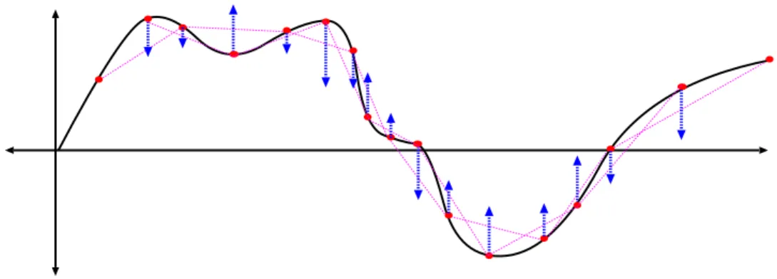
Figure 1A.1 depicts a material diffusing through a one-dimensional domain X (for example,X=R orX= [0, L]). Letu(x, t) be the density of the material at the point x∈X at time t >0. Intuitively, we expect the material to flow from regions ofgreatertolesser concentration. In other words, we expect theflowof the material at any point in space to be proportional to the slope of the curve

u(x, t) at that point. Thus, if F(x, t) is the flow at the point x at time t, then

Greyscale Landscape

u(x)

x

(26)

Grayscale Temperature Distribution

Isothermal Contours Heat Flow Vector Field

Figure 1A.2: Fourier’s Law of Heat Flow in two dimensions

we expect:

F(x, t) = −κ·∂_xu(x, t)

whereκ >0 is a constant measuring the rate of diffusion. This is an example of

Fourier’s Law.

1A(ii) ...in many dimensions

Prerequisites: §0E.

Figure 1A.2 depicts a material diffusing through a two-dimensional domain X⊂R2 (e.g. heat spreading through a region, ink diffusing in a bucket of water, etc.). We could just as easily suppose thatX⊂RD is a D-dimensional domain. If x∈ X is a point in space, and t≥ 0 is a moment in time, let u(x, t) denote the concentration atxat timet. (This determines a functionu:X×R₆₋−→R, called atime-varying scalar field.)

Now letF~(x, t) be aD-dimensional vector describing theflowof the material at the pointx∈X. (This determines atime-varying vector fieldF~ :RD×R₆₋−→ RD.)

Again, we expect the material to flow from regions of high concentration to low concentration. In other words, material should flowdown the concentration gradient. This is expressed by Fourier’s Law of Heat Flow , which says:

~

F = −κ· ∇u,

whereκ >0 is is a constant measuring the rate of diffusion.

(27)

t=4

t=5

t=6

t=7

u(x,0)

u(x,1)

u(x,2)

u(x,3)

t=0

t=1

t=2

t=3

x

u(x,4)

u(x,5)

u(x,6)

u(x,7)

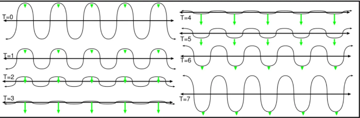
Figure 1B.1: The heat equation as “erosion”.

1B

The heat equation

Recommended: §1A.

1B(i) ...in one dimension

Prerequisites: §1A(i).

Consider a material diffusing through a one-dimensional domain X (for ex-ample, X= R or X = [0, L]). Let u(x, t) be the density of the material at the locationx∈X at timet∈R₆₋, and let F(x, t) be the flux of the material at the locationx and time t. Consider the derivative ∂xF(x, t). If ∂xF(x, t)>0, this

means that the flow is diverging1 at this point in space, so the material there is spreading farther apart. Hence, we expect the concentration at this point to decrease. Conversely, if ∂xF(x, t)<0, then the flow is converging at this point

in space, so the material there is crowding closer together, and we expect the concentration to increase. To be succinct: the concentration of material will increasein regions whereF converges, anddecreasein regions whereF diverges. The equation describing this is:

∂tu(x, t) = −∂xF(x, t).

If we combine this with Fourier’s Law, however, we get:

∂tu(x, t) = κ·∂x∂xu(x, t),

which yields theone-dimensional heat equation:

∂tu(x, t) = κ·∂x2u(x, t).

1

(28)

Heuristically speaking, if we imagineu(x, t) as the height of some one-dimensional “landscape”, then the heat equation causes this landscape to be “eroded”, as if it were subjected to thousands of years of wind and rain (see Figure 1B.1).

A) Low Frequency: Slow decay

B) High Frequency: Fast decay

Time

Figure 1B.2: Under the heat equation, the exponential decay of a periodic func-tion is proporfunc-tional to the square of its frequency.

Example 1B.1. For simplicity we suppose κ= 1.

(a) Letu(x, t) =e−9t·sin(3x). Thus,udescribes a spatially sinusoidal function (with spatial frequency 3) whose magnitude decays exponentially over time. (b) The dissipating wave: More generally, let u(x, t) = e−ω2·t_·_sin(_ω_·_x_).

Thenuis a solution to the one-dimensional heat equation, and looks like a standing wave whose amplitude decays exponentially over time (see Figure 1B.2). Notice that the decay rate of the functionu is proportional to the square of its frequency.

(c) The (one-dimensional) Gauss-Weierstrass Kernel: Let

G(x;t) := 1 2√πtexp

−x2

4t

.

Then G is a solution to the one-dimensional heat equation, and looks like a “bell curve”, which starts out tall and narrow, and over time becomes

broader and flatter (Figure 1B.3). ♦

Exercise 1B.1. Verify that the functions in Examples 1B.1(a,b,c) all satisfy the

E

(29)

Time

Figure 1B.3: The Gauss-Weierstrass kernel under the heat equation.

All three functions in Examples 1B.1 starts out very tall, narrow, and pointy, and gradually become shorter, broader, and flatter. This is generally what the heat equation does; it tends to flatten things out. If u describes a physical landscape, then the heat equation describes “erosion”.

1B(ii) ...in many dimensions

Prerequisites: §1A(ii).

More generally, if u : RD ×R₆₋ −→ R is the time-varying density of some material, and ~F : RD ×R₆₋ −→ R is the flux of this material, then we would expect the material toincrease in regions whereF~ converges, and todecreasein regions where ~Fdiverges.2 In other words, we have:

∂tu = −divF~.

Ifu is the density of some diffusing material (or heat), thenF~ is determined by

Fourier’s Law, so we get theheat equation

∂tu = κ·div∇u = κ4u.

Here,4is the Laplacian operator3_{, defined:}

4u = ∂₁2u+∂₂2u+. . . ∂_D2 u

Exercise 1B.2. (a) If D = 1, andu:R−→R, verify that div∇u(x) = u00(x) = E

4u(x), for allx∈R.

2_See_§_{0E(ii) on page 558 for a review of the ‘divergence’ of a vector field.} 3

Sometimes the Laplacian is written as “∇2

(30)

(b) If D = 2, andu: R2 −→R, verify that div∇u(x, y) = ∂2_xu(x, y) +∂_y2u(x, y) =

4u(x, y), for all (x, y)∈R2.

(c) For anyD≥2 andu:RD−→R, verify that div∇u(x) =4u(x), for allx∈RD.

By changing to the appropriate time units, we can assumeκ= 1, so theheat equationbecomes:

∂tu = 4u .

For example,

• IfX⊂R, and x∈X, then 4u(x;t) = ∂_x2u(x;t).

• IfX⊂R2, and (x, y)∈X, then4u(x, y;t) = ∂_x2u(x, y;t) +∂_y2u(x, y;t). Thus, as we’ve already seen, the one-dimensional heat equation is

∂tu = ∂x2u

and the thetwo dimensional heat equationis:

∂tu(x, y;t) = ∂x2u(x, y;t) + ∂y2u(x, y;t)

Example 1B.2.

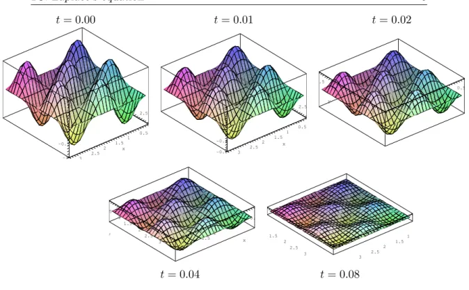
(a) Let u(x, y;t) = e−25t·sin(3x) sin(4y). Then u is a solution to the two-dimensional heat equation, and looks like a two-two-dimensional ‘grid’ of si-nusoidal hills and valleys with horizontal spacing 1/3 and vertical spacing 1/4. As shown in Figure 1B.4, these hills rapidly subside into a gently un-dulating meadow, and then gradually sink into a perfectly flat landscape. (b) The (two-dimensional) Gauss-Weierstrass Kernel: Let

G(x, y; t) := 1 4πtexp

−x2−y2

4t

.

Then G is a solution to the two-dimensional heat equation, and looks like a mountain, which begins steep and pointy, and gradually “erodes” into a broad, flat, hill.

(c) The D-dimensional Gauss-Weierstrass Kernel is the function G : RD ×R₊−→Rdefined

G(x;t) = 1

(4πt)D/2exp

− kxk2 4t

!

(31)

t= 0.00 t= 0.01 t= 0.02 0 0.5 1 _y 1.5 2 2.5 3 0 0.5 1 1.5 2 x 2.5 3 -1 -0.5 0 0.5 1 0 0.5 1 _y 1.5 2 2.5 3 0 0.5 1 1.5 2 x 2.5 3 -0.8 -0.4 0 0.4 0.8 -0.6 -0.4 -0.2 0 0.2 0 0.4 0.6 0.5 0 0.5 1 1 1.5 1.5 2 y ₂

2.5 _2.5 x

3 3 -0.3 -0.2 -0.1 0 0 0.1 0.2 0.3 0.5 0 1 0.5 1 1.5 1.5 2 2 y _2.5 2.5 x 3 3 -0.1 -0.05 0 0.05 0.1 0.5 0 1 0.5 1.5 1 1.5 2 2 2.5 2.5 3 3

t= 0.04 t= 0.08

Figure 1B.4: Five snapshots of the function u(x, y;t) = e−25t·sin(3x) sin(4y) from Example 1B.2.

Exercise 1B.3. Verify that the functions in Examples 1B.2(a,b,c) all satisfy the

E

heat equation.

Exercise 1B.4. Prove theLeibniz rulefor Laplacians: iff, g:RD−→Rare two E

scalar fields, and (f·g) :RD−→Ris their product, then for allx∈RD,

4(f·g)(x) = g(x)·4f(x) + 2∇f(x)•∇g(x) + f(x)·4g(x).

Hint: Combine the Leibniz rules for gradients and divergences (Propositions 0E.1(b)

and 0E.2(b) on pages 558 and 560).

1C

Laplace’s equation

Prerequisites: §1B.

If the heat equation describes the erosion/diffusion of some system, then an

equilibriumorsteady-stateof the heat equation is a scalar fieldh:RD −→R satisfying Laplace’s Equation:

(32)

–2 –1 0 1 2 –2

–1 0

1 2 –2

–1.5 –1 –0.5

0 0.5

–1 –0.5 0 0.5 1

x –1

–0.5 0

0.5 y –1 –0.5 0 0.5 1

–8 –6 –4 –2 0 2 4 6 8

x –3

–2 –1

0 1

2 3 y –10

–5 0 5 10

(A) (B) (C)

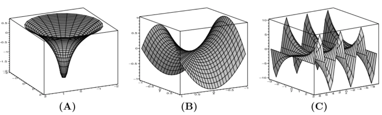
Figure 1C.1: Three harmonic functions: (A) h(x, y) = log(x2 ₊_y2_). _(B)

h(x, y) =x2−y2. (C)h(x, y) = sin(x)·sinh(y). In all cases, note the telltale “saddle” shape.

A scalar field satisfying the Laplace equation is called aharmonic function.

Example 1C.1.

(a) If D = 1, then 4h(x) = ∂_x2h(x) = h00(x); thus, the one-dimensional Laplace equationis just

h00(x) = 0

Supposeh(x) = 3x+ 4. Thenh0(x) = 3, andh00(x) = 0, so h is harmonic. More generally: the one-dimensional harmonic functions are just thelinear functions of the form: h(x) =ax+b for some constantsa, b∈R.

(b) IfD= 2, then4h(x, y) =∂_x2h(x, y) +∂_y2h(x, y), so thetwo-dimensional Laplace equationreads:

∂_x2h+∂2_yh = 0,

or, equivalently,∂_x2h=−∂_y2h. For example:

• Figure 1C.1(B) shows the harmonic functionh(x, y) =x2₋_y2_.

• Figure 1C.1(C) shows the harmonic functionh(x, y) = sin(x)·sinh(y).

Exercise 1C.1 Verify that these two functions are harmonic. ♦ E

(33)

Example 1C.2. Figure 1C.1(A) shows the harmonic functionh(x, y) = log(x2+

y2) for all (x, y) 6= (0,0). This function is well-defined everywhere except at (0,0); hence, contrary to appearances, (0,0) isnotan extremal point. [Verifying

thathis harmonic is problem # 3 on page 20]. ♦

When D ≥ 3, harmonic functions no longer define nice saddle-shaped sur-faces, but they still have similar mathematical properties.

Example 1C.3.

(a) IfD= 3, then 4h(x, y, z) = ∂_x2h(x, y, z) +∂_y2h(x, y, z) +∂_z2h(x, y, z). Thus, thethree-dimensional Laplace equationreads:

∂_x2h+∂_y2h+∂_z2h = 0,

For example, let h(x, y, z) = 1

k(x, y, z)k =

1

p

x2₊_y2₊_z2 for all

(x, y, z)6= (0,0,0). Thenh is harmonic everywhere except at (0,0,0).

[Verifying thathis harmonic is problem # 4 on page 21.]

(b) For anyD≥3, theD-dimensional Laplace equation reads:

∂₁2h+. . .+∂_D2 h = 0.

For example, let h(x) = 1 kxkD−2 =

1

x2

1+· · ·+x2D

D−₂2

for all x6= 0. Thenh is harmonic everywhere everywhere in RD\ {0} (Exercise 1C.2 E

Verify thathis harmonic onRD\ {0}.) ♦

Harmonic functions have the convenient property that we can multiply to-gether two lower-dimensional harmonic functions to get a higher dimensional one. For example:

• h(x, y) = x·y is a two-dimensional harmonic function (Exercise 1C.3 E

Verify this).

• h(x, y, z) =x·(y2−z2) is a three-dimensional harmonic function (Exercise 1C.4

Verify this). E

(34)

Proposition 1C.4. Suppose u:Rn −→ Ris harmonic and v :Rm −→ Ris

harmonic, and define w:Rn+m −→ R by w(x,y) =u(x)·v(y) for x∈Rn and

y∈Rm. Thenw is also harmonic

Proof. Exercise 1C.5 Hint: First prove that w obeys a kind of Leibniz rule: E

4w(x,y) = v(y)· 4u(x) +u(x)· 4v(y). 2

The function w(x,y) = u(x)·v(y) is called a separated solution, and this theorem illustrates a technique called separation of variables. The next exercise also explores separation of variables. A full exposition of this technique appears in Chapter 16 on page 353.

Exercise 1C.6. (a) Letµ, ν ∈Rbe constants, and letf(x, y) = eµx·eνy. Suppose

E

f is harmonic; what can you conclude about the relationship betweenµandν? (Justify your assertion).

(b) Suppose f(x, y) = X(x)·Y(y), where X :R−→Rand Y :R−→Rare two smooth functions. Supposef(x, y) is harmonic

[i] Prove that X

00₍_x₎

X(x) =

−Y00(y)

Y(y) for allx, y∈R.

[ii] Conclude that the function X

00₍_x₎

X(x) must equal a constant c independent of x. HenceX(x) satisfies the ordinary differential equationX00(x) =c·X(x).

Likewise, the function Y

00₍_y₎

Y(y) must equal−c, independent ofy. HenceY(y) satisfies the ordinary differential equationY00(y) =−c·Y(y).

[iii] Using this information, deduce the general form for the functionsX(x) andY(y), and use this to obtain a general form forf(x, y).

1D

The Poisson equation

Prerequisites: §1C.

Imagine p(x) is the concentration of a chemical at the point x in space. Suppose this chemical is being generated (or depleted) at different rates at dif-ferent regions in space. Thus, in the absence of diffusion, we would have the

generation equation

∂tp(x, t) = q(x),

whereq(x) is the rate at which the chemical is being created/destroyed atx(we assume thatq is constant in time).

If we now included the effects of diffusion, we get thegeneration-diffusion equation:

(35)

0 0.2 0.4 0.6 0.8 1 1.2 1.4 1.6

0 0.5 1 1.5 2

p"(x)

p’(x)

p(x)

-20 -15 -10 -5 0 5 10 15 20

-3 -2 -1 0 1 2 3

p’(x)

p(x)

p’’(x)

p’(x)

p00₍_x_{) =}_Q₍_x_{) =}

1 if 0< x <1;

0 otherwise. p

00₍_x_{) =}_Q₍_x_{) = 1}_/x2_;

p0(x) =

x if 0< x <1;

1 otherwise. p

0₍_x_{) =}₋₁_/x_{+ 3;}

p(x) =

x2_/₂ _{if 0}_{< x <}_1; x−1

2 otherwise.

p(x) =−log|x|+ 3x+ 5.

(A) (B)

Figure 1D.1: Two one-dimensional potentials.

Asteady stateof this equation is a scalar fieldpsatisfyingPoisson’s Equation:

4p=Q.

whereQ(x) = −q(x)

κ .

Example 1D.1: One-Dimensional Poisson Equation

IfD= 1, then4p(x) =∂_x2p(x) =p00(x); thus, theone-dimensional Poisson equationis just

p00(x) =Q(x).

We can solve this equation by twice-integrating the function Q(x). If p(x) =

R R

Q(x) is some double-antiderivative ofG, thenpclearly satisfies the Poisson equation. For example:

(a)Suppose Q(x) =

1 if 0< x <1;

0 otherwise. . Then define

p(x) =

Z x

0

Z y

0

q(z)dz dy =







0 if x <0;

x2/2 if 0< x <1;

x−1₂ if 1< x.

(Figure 1D.1A)

(b) If Q(x) = 1/x2 _(for_x _{6= 0), then} _p₍_x_{) =} R R

Q(x) = −log|x|+ax+b

(36)

–10 –5

0 5

10 –10

–5

0

5

10 –2

–1.5 –1 –0.5

0 0.5

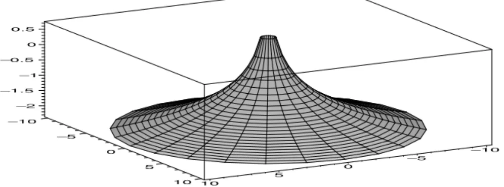
Figure 1D.2: The two-dimensional potential field generated by a concentration of charge at the origin.

Exercise 1D.1. Verify that the functionsp(x) in Examples (a) and (b) are both

E

solutions to their respective Poisson equations.

Example 1D.2: Electrical/Gravitational Fields

Poisson’s equation also arises in classical field theory4. Suppose, for any point

x = (x1, x2, x3) in three-dimensional space, that q(x) is charge density at x,

and thatp(x) is the the electric potential field atx. Then we have:

4p(x) = κ q(x) (κ some constant) (1D.1) If q(x) were the mass density at x, and p(x) were the gravitational potential energy, then we would get the same equation. (See Figure 1D.2 for an example of such a potential in two dimensions).

In particular, in a region where there is no charge/mass (i.e. where q ≡ 0), equation (1D.1) reduces to the Laplace equation 4p ≡ 0. Because of this, solutions to the Poisson equation (and especially the Laplace equation) are

sometimes called potentials. ♦

Example 1D.3: The Coulomb Potential

Let D= 3, and let p(x, y, z) = 1

k(x, y, z)k =

1

p

x2₊_y2₊_z2. In Example

1C.3(a), we asserted thatp(x, y, z) was harmonic everywhere except at (0,0,0), where it is not well-defined. For physical reasons, it is ‘reasonable’ to write the equation:

4p(0,0,0) = δ0, (1D.2)

4

(37)

where δ0 is the ‘Dirac delta function’ (representing an infinite concentration

of charge at zero)5. Then p(x, y, z) describes the electric potential generated

by a point charge. ♦

Exercise 1D.2. Check that ∇p(x, y, z) = −(x, y, z)

k(x, y, z)k3. This is the electric field E

generated by a point charge, as given byCoulomb’s Lawfrom classical electrostatics.

Exercise 1D.3. (a) Let q :R3−→R be a scalar field describing a charge density E

distribution. If E~ : R3 −→ R3 is the electric field generated by q, thenGauss’s law saws divE~ =κ q, where κ is a constant. If p: R3 −→R is the electric potential field associated withE, then by definition,~ ~E=∇p. Use these facts to derive equation (1D.1). (b) Supposeqis independent of thex3coordinate; that is,q(x1, x2, x3) =Q(x1, x2) for some functionQ:R2−→R. Show thatpis also is independent of thex₃coordinate; that is,p(x1, x2, x3) =P(x1, x2) for some functionP :R2−→R. ShowP andQsatisfy thetwo-dimensional version of the Poisson equation —that is that 4P = κ Q.

(This is significant because many physical problems have (approximate) translational symmetry along one dimension (e.g. an electric field generated by a long, uniformly charged wire or plate). Thus, we can reduce the problem to two dimensions, where powerful methods from complex analysis can be applied; see Section 18B on page 422.)

Notice that the electric/gravitational potential field is not uniquely defined by equation (1D.1). If p(x) solves the Poisson equation (1D.1), then so does

e

p(x) = p(x) +a for any constant a ∈ R. Thus, we say that the potential field is well-defined up to addition of a constant; this is similar to the way in which the antiderivativeR Q(x) of a function is only well-defined up to some constant.6 This is an example of a more general phenomenon:

Proposition 1D.4. Let X⊂RD be some domain, and let p :X−→ R and

h : X −→ R be two functions on X. Let

e

p(x) := p(x) +h(x) for all x ∈ X.

Suppose that h is harmonic —i.e. 4h ≡ 0. If p satisfies the Poisson Equation

“4p≡q”, then p_ealso satisfies this Poisson equation.

Proof. Exercise 1D.4 Hint: Notice that4pe(x) =4p(x) +4h(x). 2 E

For example, ifQ(x) = 1/x2, as in Example 1D.1(b), thenp(x) =−log(x) is a solution to the Poisson equation “p00(x) = 1/x2”. If h(x) is a one-dimensional

5_{Equation (1D.2) seems mathematically nonsensical, but it} _can _{be made mathematically}

meaningful, usingdistribution theory. However, this is far beyond the scope of this book, so for our purposes, we will interpret eqn. (1D.2) as purely metaphorical.

6

For the purposes of the physical theory, this constantdoes not matter, because the field

(38)

harmonic function, thenh(x) =ax+bfor some constantsaandb(see Example 1C.1(a) on page 10). Thusp_e(x) =−log(x) +ax+b, and we’ve already seen that these are also valid solutions to this Poisson equation.

1E

Properties of harmonic functions

Prerequisites: §1C,§0H(ii). Prerequisites(for proofs): §2A,§17G,§0E(iii).

Recall that a function h : RD −→ R is harmonic if 4h ≡ 0. Harmonic functions have nice geometric properties, which can be loosely summarized as ‘smooth and gently curving’.

Theorem 1E.1. Mean Value Theorem

Let f : RD −→ R be a scalar field. Then f is harmonic if and only if f is

integrable, and:

For anyx∈RD, and any R >0, f(x) = 1

A(R)

Z

S(x;R)

f(s) ds. (1E.1)

Here, S(x;R) := s∈RD ; ks−xk=R is the (D−1)-dimensional sphere of

radiusR aroundx, andA(R) is the(D−1)-dimensional surface area ofS(x;R). Proof. Exercise 1E.1 (a) Suppose f is integrable and statement (1E.1) is true.

E

Use theSpherical Meansformula for the Laplacian (Theorem 2A.1) to show that

f is harmonic.

(b) Now, supposefis harmonic. Defineφ:R₆₋−→Rby: φ(R) := 1 A(R)

Z

S(x;R)

f(s)ds.

Show thatφ0(R) = K

A(R)

Z

S(x;R)

∂_⊥f(s)ds, for some constantK >0.

Here, ∂⊥f(s) is theoutward normal derivativeoff at the point son the sphere (see page 564 for an abstract definition; see§5C(ii) on page 76 for more information).

(c) LetB(x;R) :=b∈RD; kb−xk ≤R be theballof radiusRaroundx. Apply

Green’s Formula(Theorem 0E.5(a) on page 564) to show that

φ0(R) = K

A(R)

Z

B(x;R)

4f(b)db.

(d) Deduce that, iff is harmonic, thenφmust be constant.

(e) Use the fact that f is continuous to show that lim

r→0φ(r) = f(x). Deduce that φ(r) = f(x) for all r ≥ 0. Conclude that, if f is harmonic, then statement (1E.1)

(39)

Corollary 1E.2. Maximum Principle for harmonic functions

Let X ⊂ RD be a domain, and let u : X −→ R be a nonconstant harmonic

function. Thenuhas no local maximal or minimal points anywhere in the interior ofX.

If Xis bounded(hence compact), thenu doesobtain a maximum and

mini-mum, but only on the boundaryof X.

Proof. (by contradiction). Supposexwasa local maximum ofusomewhere in the interior ofX. LetR >0 be small enough thatS(x;R)⊂X, and such that

u(x) ≥ u(s) for alls∈S(x;R), (1E.2) where this inequality is strict for at least one s0 ∈S(x;R).

Claim 1: There is a nonempty open subsetY⊂S(x;R) such that u(x) >

u(y) for all yinY.

Proof. We know thatu(x)> u(s0). But u is continuous, so there must be

some open neighbourhood Y around s0 such that u(x) > u(y) for all y in

Y.

Claim 1 Equation (1E.2) and Claim 1 imply that

f(x) > 1 A(R)

Z

S(x;R)

f(s) ds.

But this contradicts the Mean Value Theorem. By contradiction,xcannot be a local maximum. (The proof for local minima is analogous). 2

A function F :RD −→ R is spherically symmetricif F(x) depends only on the norm kxk (i.e. F(x) = f(kxk) for some function f : R₆₋ −→ R). For example, the function F(x) := exp(− kxk2) is spherically symmetric.

If h, F :RD −→ R are two integrable functions, then their convolution is the functionh∗F :RD −→Rdefined by

h∗F(x) :=

Z

RD

h(y)·F(x−y) dy, for allx∈RD

(if this integral converges). We will encounter convolutions in § 10D(ii) on page 214 (where they will be used to prove theL2 convergence of a Fourier series) and again in Chapter 17 (where they will be used to construct ‘impulse-response’ solutions for PDEs). For now, we state the following simple consequence of the Mean Value Theorem:

Lemma 1E.3. If h :RD −→ R is harmonic and F :RD −→R is integrable

and spherically symmetric, then h∗F =K·h, whereK∈Ris some constant.

(40)

Proposition 1E.4. Smoothness of harmonic functions

If h:RD −→R is a harmonic function, then his infinitely differentiable. Proof. Let F :RD −→ R be some infinitely differentiable, spherically

sym-metric, integrable function. For example, we could take F(x) := exp(− kxk2). Then Proposition 17G.2(f) on page 410 says that h∗F is infinitely differen-tiable. But Lemma 1E.3 implies that h∗F =Kh for some constantK ∈R; thus, his also infinitely differentiable.

(For another proof, see Theorem 6 on p. 28 of [Eva91,§2.2].) 2

Actually, we can go even further than this. A function h : X −→ R is

analyticif, for every x∈X, there is a multivariate Taylor series expansion for

h aroundxwith a nonzero radius of convergence.7

Proposition 1E.5. Harmonic functions are analytic

Let X⊆ RD be an open set. If h :X −→ R is a harmonic function, then h is

analytic onX.

Proof. For the caseD= 2, see Corollary 18D.2 on page 451. For the general case D≥2, see Theorem 10 on p. 31 of [Eva91,§2.2]. 2

1F

∗

Transport and diffusion

Prerequisites: §1B,§6A.

If u : RD −→ R is a “mountain”, then recall that ∇u(x) points in the direction of most rapid ascentatx. If~v∈RD is a vector, then the dot product

~v•∇u(x) measures how rapidly you would be ascending if you walked in direction

~v.

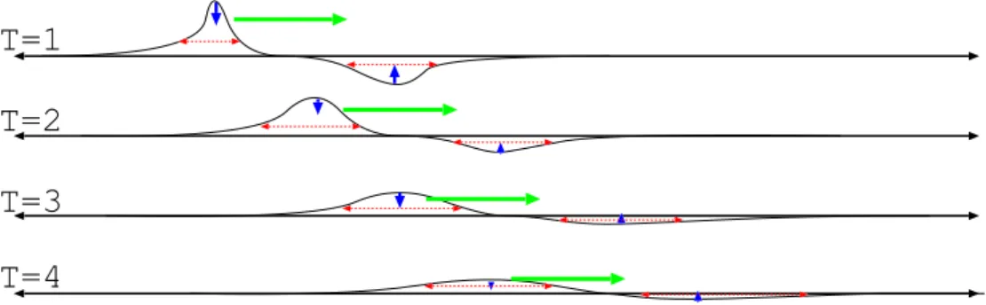
Suppose u :RD −→ R describes a pile of leafs, and there is a steady wind blowing in the direction ~v ∈ RD. We would expect the pile to slowly move in the direction~v. Suppose you were an observer fixed at location x. The pile is moving past you in direction~v, which is the same as you walking along the pile in direction −~v; thus, you would expect the height of the pile at your location to increase/decrease at rate−~v• ∇u(x). The pile thus satisfies theTransport Equation:

∂tu = −~v• ∇u.

Now, suppose that the wind does not blow in aconstant direction, but instead has some complex spatial pattern. The wind velocity is therefore determined by avector field V~ :RD −→ RD. As the wind picks up leafs and carries them around, thefluxof leafs at a pointx∈Xis then the vectorF~(x) =u(x)·V~(x).

7

(41)

1G. Reaction and diffusion 19 But the rate at which leafs are piling up at each location is thedivergenceof the flux. This results inLiouville’s Equation:

∂tu = −divF~ = −div (u·V~) ₍_∗₎ −V~ • ∇u − u·divV~.

Here, (∗) is by the Leibniz rule for divergence (Proposition 0E.2(b) on page 560). Liouville’s equation describes the rate at whichu-material accumulates when it is being pushed around by the V~-vector field. Another example: V~(x) de-scribes the flow of water at x, and u(x) is the buildup of some sediment at

x.

Now suppose that, in addition to the deterministic force V~ acting on the leafs, there is also a “random” component. In other words, while being blown around by the wind, the leafs are also subject to some random diffusion. To describe this, we combineLiouville’s Equationwith theheat equation, to obtain theFokker-Plank equation:

∂tu = κ4u − V~ • ∇u − u·divV~.

1G

∗

Reaction and diffusion

Prerequisites: §1B.

SupposeA,B and C are three chemicals, satisfying the chemical reaction: 2A+B =⇒ C

As this reaction proceeds, theAandB species are consumed, andCis produced. Thus, ifa,b,care the concentrations of the three chemicals, we have:

∂tc = R(t) = −∂tb = −

1 2∂ta,

whereR(t) is the rate of the reaction at time t. The rateR(t) is determined by the concentrations ofAandB, and by a rate constantρ. Each chemical reaction requires 2 molecules ofA and one of B; thus, the reaction rate is given by

R(t) = ρ·a(t)2·b(t)

Hence, we get three ordinary differential equations, called thereaction kinetic equationsof the system:

∂ta(t) = −2ρ·a(t)2·b(t)

∂tb(t) = −ρ·a(t)2·b(t)

∂tc(t) = ρ·a(t)2·b(t)







(1G.1)

(42)

concentration ofB andc(x, t) be the concentration ofC. (This determines three time-varying scalar fields, a, b, c :R3×R−→ R.) As the chemicals react, their concentrations at each point in space may change. Thus, the functionsa, b, cwill obey the equations (1G.1) at each point in space. That is, for everyx∈R3 and

t∈R, we have

∂ta(x;t) ≈ −2ρ·a(x;t)2·b(x;t)

etc. However, the dissolved chemicals are also subject todiffusionforces. In other words, each of the functions a, b and c will also be obeying the heat equation. Thus, we get the system:

∂ta = κa· 4a(x;t) − 2ρ·a(x;t)2·b(x;t)

∂tb = κb· 4b(x;t) − ρ·a(x;t)2·b(x;t)

∂tc = κc· 4c(x;t) + ρ·a(x;t)2·b(x;t)

whereκa, κb, κc >0 are three different diffusivity constants.

This is an example of a reaction-diffusion system. In general, in a reaction-diffusion system involving N distinct chemicals, the concentrations of the different species is described by aconcentration vector field u:R3×R−→ RN, and the chemical reaction is described by arate functionF :RN −→RN. For example, in the previous example,u(x, t) =a(x, t), b(x, t), c(x, t), and

F(a, b, c) = −2ρa2b, −ρa2b, ρa2b.

Thereaction-diffusion equations for the system then take the form

∂tun = κn4un + Fn(u),

forn= 1, ..., N

1H

Practice problems

1. Letf :R4 −→Rbe a differentiable scalar field. Show that div∇f(x₁, x₂, x₃, x₄) = 4f(x1, x2, x3, x4).

2. Letf(x, y;t) = exp(−34t)·sin(3x+ 5y). Show thatf(x, y;t) satisfies the two-dimensional heat equation: ∂tf(x, y;t) = 4f(x, y;t).

3. Letu(x, y) = log(x2+y2). Show thatu(x, y) satisfies the (two-dimensional) Laplace Equation, everywhere except at (x, y) = (0,0).

Remark: If (x, y)∈R2, recall thatk(x, y)k :=

p

x2₊_y2_{. Thus, log(}_x2₊

Linear Partial Differential Equations and Fourier Theory - Free Computer, Programming, Mathematics, Technical Books, Lecture Notes and Tutorials