Cover Page
The handle http://hdl.handle.net/1887/21760 holds various files of this Leiden University dissertation.
Exceptional Model Mining
Proefschrift
ter verkrijging van
de graad van Doctor aan de Universiteit Leiden, op gezag van Rector Magnificus prof.mr. C.J.J.M. Stolker,
volgens besluit van het College voor Promoties te verdedigen op dinsdag 17september 2013
klokke 11.15 uur
door
Wouter Duivesteijn
Promotor: prof. dr. J. N. Kok
Co-promotor: dr. A. J. Knobbe
Overige leden: prof. dr. P. A. Flach (University of Bristol)
prof. dr. H. Blockeel (Katholieke Universiteit Leuven) dr. W. A. Kosters
Cover photo: ochre sea stars (Pisaster ochraceus), taken at Ganges Har-bour, Salt Spring Island, British Columbia, Canada. Licensed under the Creative Commons Attribution-Share Alike 3.0 Unported license by D. Gordon E. Robertson.
Contents
1 Introduction 1
1.1 Overview . . . 4
2 Motivation and Preliminaries 7 2.1 Preliminaries . . . 10
3 The Exceptional Model Mining Framework 13 3.1 Search Strategy . . . 15
3.1.1 Refinement Operator and Description Language . . 16
3.1.2 Beam Search Algorithm for Top-q EMM . . . 18
3.1.3 Alternatives to Beam Search . . . 21
3.2 How to Define an EMM Instance? . . . 22
3.2.1 Quality Measure Concepts . . . 22
3.2.2 Compared to what? . . . 24
3.3 Related Work . . . 26
3.3.1 Search Strategies for SD/EMM . . . 26
3.3.2 Similar Local Pattern Mining Tasks . . . 27
3.3.3 Similar Tasks with a Broader Scope . . . 29
3.4 Software . . . 31
4 Deviating Interactions – Correlation Model 33 4.1 Quality Measure ϕscd . . . 33
4.2 Experiments . . . 34
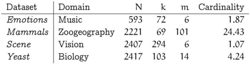
4.2.1 Datasets . . . 34
4.2.2 Experimental Results . . . 35
4.3 Alternatives . . . 38
4.4 Conclusions . . . 40
5 Deviating Predictive Performance – Classification Model 41
5.1 Quality Measure ϕsed. . . 42
5.2 Experiments . . . 42
5.2.1 Datasets . . . 42
5.2.2 Experimental Results . . . 42
5.3 Alternatives . . . 43
5.3.1 BDeu Score (ϕBDeu) . . . 44
5.3.2 Hellinger (ϕHel) . . . 44
5.3.3 Experimental Results . . . 45
5.4 Conclusions . . . 47
6 Unusual Conditional Interactions – Bayesian Network Model 49 6.1 Quality Measure ϕweed . . . 50
6.1.1 Independence Relations in Bayesian Networks . . . . 51
6.1.2 Edit Distance for Bayesian Networks . . . 52
6.2 Experiments . . . 54
6.2.1 Datasets . . . 54
6.2.2 Experimental Results . . . 55
6.3 Alternatives . . . 63
6.4 Conclusions . . . 66
7 Different Slopes for Different Folks – Regression Model 69 7.1 Quality Measure ϕCook . . . 70
7.2 Experiments . . . 73
7.2.1 Datasets . . . 73
7.2.2 Experimental Results . . . 76
7.3 Pruning with Bounds for Cook’s Distance . . . 80
7.3.1 Empirical bound evaluation . . . 83
7.4 Alternatives . . . 86
7.5 Conclusions . . . 87
8 Exploiting False Discoveries – Validating Found Descriptions 91 8.1 Problem Statement . . . 92
8.2 Validation Method . . . 93
8.2.1 Randomization Techniques . . . 94
8.2.2 Building a Statistical Model . . . 96
CONTENTS vii
8.3 Experiments . . . 97
8.3.1 Validating Descriptions . . . 101
8.3.2 Validating Quality Measures . . . 102
8.3.3 Validating EMM Results . . . 105
8.4 Discussion . . . 107
8.4.1 Validating Descriptions . . . 108
8.4.2 Validating Quality Measures . . . 108
8.4.3 Validating EMM Results . . . 110
8.5 Related Work . . . 110
8.6 Conclusions . . . 112
9 Multi-label LeGo – Enhancing Multi-label Classifiers with Local Patterns 115 9.1 The LeGo Framework . . . 116
9.2 Multi-label Classification . . . 118
9.3 LeGo Components . . . 120
9.3.1 Local Pattern Mining Phase . . . 120
9.3.2 Pattern Subset Discovery Phase . . . 120
9.3.3 Global Modeling Phase . . . 122
9.4 Experimental Setup . . . 123
9.4.1 Evaluation Measures . . . 124
9.4.2 Statistical Testing . . . 125
9.5 Experimental Evaluation . . . 126
9.5.1 Feature Selection Methods . . . 126
9.5.2 Evaluation of the LeGo Approach . . . 127
9.5.3 Evaluation of the Decompositive Approaches . . . . 131
9.5.4 Efficiency . . . 133
9.6 Discussion and Related Work . . . 134
9.7 Conclusions . . . 136
10 Conclusions 139
References 145
Nederlandse Samenvatting 157
English Summary 159
Acknowledgments 161
Chapter 1
Introduction
In their seminal 1996 paper [30], Fayyad, Piatetsky-Shapiro, and Smyth outlined their view on data mining, and what they called KDD, the then-emerging field ofKnowledge Discovery in Databases. The basic problem that KDD strives to solve is the following: when presented with a set of raw data (which is usually too voluminous to inspect manually), distill in-formation out of that dataset that is more compact, more abstract, or more useful. The authors wrote: “KDD is an attempt to address a problem that the digital information era made a fact of life for all of us: data overload.” Since then, the internet has evolved from an additional source of infor-mation that we would occasionally dial into, to an always available vital necessity. Add to that the recent smartphone penetration into everyone’s daily life, and we see that every person and company in the world gener-ates more and more data. Hence the need for KDD methods has become evermore pressing.
Fayyad et al. divide the KDD process into nine stages, the seventh of which is Data Mining. After understanding the application domain, creating a dataset, cleaning and projecting the dataset, hypothesis selection and a few other preparatory steps, we arrive at the stage where we can search within a given dataset for “patterns of interest in a particular representational form or a set of such representations”, before going to subsequent stages where patterns are interpreted and acted upon. In this dissertation we are mainly occupied with a subfield of data mining (the seventh stage of KDD), with some additional pattern interpretation (the eighth stage of KDD).
In the data mining phase, a given dataset is assumed. One can distinguish several methods to mine the dataset. The following were discussed by Fayyad et al.
Classification: mapping records of the dataset into one or several classes;
Regression: mapping records of the dataset to a real-valued prediction vari-able;
Clustering: identifying a finite set of categories to describe the dataset;
Summarization: finding a compact description for a subset of the dataset;
Dependency Modeling: finding a model that describes significant dependen-cies between variables;
Change and Deviation Detection: discovering substantial deviations in the data from the normative, or from previously measured values.
The data mining task we consider in this dissertation combines aspects of the last three methods, and has an application in the first.
The goal of Local Pattern Mining (LPM) is to find subsets of the dataset at hand, that are interesting in some sense. The goal is not to partition the dataset, and not to classify the dataset. We rather strive to pinpoint multiple (potentially overlapping) interesting subsets at the same time. The interestingness of a subset is gauged without considering the (lack of) coherence of records in the complement of the dataset, and without considering to what extent its interestingness is already represented by other found subsets: subsets are judged purely on their own merit. In LPM we are not quite interested in just any subset of the dataset; we are usually striving to find subgroups: subsets of the dataset that can be succinctly described in terms of conditions on attributes of the dataset. In this respect, LPM resembles the Summarization method introduced above. Originally, LPM was introduced as an unsupervised task where the interestingness
was measured in terms of an unusually high frequency of a co-occurrence. In terms of such an interestingness definition, LPM resembles theDeviation Detection method introduced above.
3
this target has an unusual distribution. Exceptionality of the distribution is usually gauged in terms of the relative frequencies of target values within the subgroup, compared to these frequencies on the whole dataset, and in terms of the size of the subgroup.
Unsupervised Local Pattern Mining (finding subgroups based on high fre-quency) and Subgroup Discovery (finding subgroups based on the distribu-tion of one target) are interesting tasks. However, they do not encompass all possible forms of “interesting” subgroups of the dataset. In this disser-tation we introduce theExceptional Model Mining (EMM) framework, to accomodate a more general form of interestingness. In the EMM frame-work, the attributes of the dataset are partitioned into two: one part (the
descriptors) is used to define subgroups on, and one part (the targets) is used to evaluate subgroups on. The concept of interest in subgroups is captured by learning, from (a subset of) the dataset, amodel fitted on the targets. The goal of EMM in general is to find subgroups for which the model learned from the records belonging to the subgroup, has parameters that deviate substantially from the parameters of the model learned from the whole dataset. Alternatively, one can compare with the model learned from the complement of the subgroup; this choice will be discussed in de-tail in Section 3.2.2. EMM is instantiated by selecting two things: amodel class, which indicates the type of interplay between targets we strive to find deviations for, and a quality measure, which quantifies the dissimi-larity between two models from the model class. Striving to find unusual interplay between several targets, is where EMM resembles theDependency Modeling method introduced by Fayyad et al.
1.1
Overview
This dissertation consists of ten chapters, of which this introduction is the first. In this section, we shortly outline the remaining chapters, discussing the previous publications on which they are based, and giving the appro-priate credits to (co-)authors.
In Chapter 2: Motivation and Preliminaries, we give motivating examples for Exceptional Model Mining, and introduce some notation. The examples have been discussed before in publications [23] and [25].
InChapter 3: The Exceptional Model Mining Framework, we introduce the gen-eral Exceptional Model Mining framework. The EMM concept, including the introduction of the refinement operator, has appeared before in a paper by D. Leman, A. Feelders, and A. Knobbe, published in the proceedings of the European Conference on Machine Learning and Principles and Prac-tice of Knowledge Discovery in Databases (ECML/PKDD 2008) [71]. The remainder of Chapter3, discussing our choices for the refinement operator and description language, algorithm and complexity analysis, how to define an EMM instance, related work, and the used software, is new.
The four subsequent chapters all introduce one choice of model class for EMM. None of these chapters explicitly discuss related work; since they instantiate the general framework of Chapter 3, we discuss all relevant related work there.
In Chapter 4: Deviating Interactions – Correlation Model, we discuss the EMM instance with the correlation between two numeric targets as model class. The original idea for this model class was first published by D. Leman, A. Feelders, and A. Knobbe, in the proceedings of the European Conference on Machine Learning and Knowledge Discovery in Databases (ECML / PKDD 2008) [71]. In Chapter 4, we reinterpret their work, and put it in the more general EMM context.
1.1. OVERVIEW 5
InChapter 6: Unusual Conditional Interactions – Bayesian Network Model, we dis-cuss the EMM instance with a Bayesian network on several nominal targets as model class. This work was published by W. Duivesteijn, A. Knobbe, A. Feelders, and M. van Leeuwen, in the proceedings of the 10th IEEE International Conference on Data Mining (ICDM2010) [25].
In Chapter 7: Different Slopes for Different Folks – Regression Model, we dis-cuss the EMM instance with a linear regression model on multiple targets as model class. In addition to the standard content of an EMM instance chapter, this chapter also contains a discussion of pruning the EMM search space with bounds on the developed quality measure. This work was pub-lished by W. Duivesteijn, A. Feelders, and A. Knobbe, in the proceedings of the 18th ACM SIGKDD Conference on Knowledge Discovery and Data Mining (KDD 2012) [23]. The idea for the simpler, alternative model class described in Section 7.4 was first published by D. Leman, A. Feelders, and A. Knobbe [71]; its interpretation and contextualization are new.
Having discussed Exceptional Model Mining instances, the following two chapters are dedicated to a related and an extended task. Contrary to the preceding four chapters, these following two chapters do come with their own related work discussions.
In Chapter 8: Exploiting False Discoveries – Validating Found Descriptions, we develop a method to determine the statistical significance of the outcome of supervised Local Pattern Mining tasks, such as Exceptional Model Mining. The quality of found descriptions is gauged against a model built over artificially generated false discoveries, to refute the hypothesis that a found description is also a false discovery. This method is additionally used to objectively compare different quality measures for the same task, by virtue of their capability to distinguish true from false discoveries. This work was published by W. Duivesteijn and A. Knobbe, in the proceedings of the11th IEEE International Conference on Data Mining (ICDM 2011) [24].
what elevates a multi-label classifier over multiple single-label classifiers. Hence, employing the descriptions as binary attributes for a multi-label classifier should improve classifier performance. In this chapter we discuss the extent to which this LeGo approach [37, 57] indeed improves per-formance. This work was published by W. Duivesteijn, E. Loza Mencía, J. Fürnkranz, and A. Knobbe, in the proceedings of the11th International Symposium on Intelligent Data Analysis (IDA 2012) [26]. An extended version was published by the same authors as a technical report of the Technische Universität Darmstadt [27]. This being joint work involving another PhD student, two reinterpretations and contextualizations of pub-lications [26] and [27] are available. The one is Chapter 9 of this disserta-tion, and the other has appeared as a chapter in the Ph.D. dissertation of E. Loza Mencía [73].
Chapter 2
Motivation and Preliminaries
Finding elements that behave differently from the norm in a dataset is a task of paramount importance. Most data mining research in this direction focuses on detecting outliers: simply identifying the peculiarly-behaving records. The characteristic feature of local pattern mining techniques that separates them from such outlier detection methods, is that in local pattern mining, we are not just looking for any outlying record or set of records in the data. Instead, we are looking for subgroups: coherent subsets for which we can formulate a concise description in terms of conditions on attributes of the data. The existence of such descriptions makes the subgroups more actionable: if we can tell a drug manufacturer that ten of his patients react badly to a certain type of medication, this doesn’t help him much, but if we can tell him instead that the group of smokers under the age of thirty react badly, this gives the manufacturer a clear indication in which direction to find a solution to his problem.
When the target concept in a dataset can no longer be captured by one particular attribute, but we still want to find exceptional subgroups in the dataset, we find a need for Exceptional Model Mining. As an example of a relatively complex target concept, consider the research performed by Robert T. Paine in 1963 and 1964 in Makah Bay, Washington [86]. It concerns the carnivore starfish Pisaster ochraceus whose presence kept a marine ecosystem consisting of 15 species stable. In this system, the spongeHaliclona was browsed upon by the nudibranchAnisodoris. When
Pisaster was artificially removed, the bivalve Mytilus californianus and
the barnacles Balanus glandula andMitella polymerus rapidly grew and crowded out other species. In total, only 8 species remained. Also, the sponge-nudibranch food chain was displaced, and the anemone population was reduced in density. Counterintuitively, when present,Pisaster did not eat any of these last three species.
In the studied ecosystem, Pisaster was the top carnivore: it consumed other species, but no other species consumed him, and Pisaster was the only species in the system for which both these statements held. This made Paine et al.’s research very relevant from a biological point of view; up until that point, it was generally assumed that removing the top carnivore from an ecosystem would increase diversity, but thePisaster experiment proved that that was not necessarily the case.
Paine remarks that the food chains are strongly influenced byPisaster, but by an indirect process. When dealing with a dataset detailing the presence of individual species, existing methods can probably detect simple patterns in the ecosystem, such as the growth ofMytilus,Balanus andMitella and the decline in the number of species when Pisaster is removed. However, the more indirect influence ofPisaster on processes such as a food chain it is not direcly related to, for instance between Haliclona and Anisodoris, cannot be found by looking at single species or even correlations between pairs of species: the (in-)dependence between Haliclona and Anisodoris
is conditional on the presence ofPisaster.
Paine models the food chains in the ecosystem as a Bayesian network. In order to find subgroups where the food chains between species are sub-stantially different from the norm, we need to be able to detect the in-direct processes that can be captured with a Bayesian network. Using an Exceptional Model Mining instance, we can for instance find subgroups defined by environmental parameters in which complex food chains are dis-placed. The ability to cope with Bayesian networks makes the same EMM instance applicable to datasets from such diverse fields as information re-trieval [9], traffic accident reconstruction [18], medical expert systems [20], gene expression in computational biology [33], and financial operational risk [82].
9
paradox for regression models. The economic law of demand states that, all else equal, if the price of a good increases, the demand for the product will decrease. Sir Robert Giffen described conditions under which this law does not hold [77]. The classic example concerns extremely poor households, who mainly consume cheap staple food, and relatively rich households in the same neighborhood, who can afford to enrich their meals with a luxury food. In this situation, when the price of the staple food increases, there will be a point where the relatively rich households can no longer afford the luxury food. These people need to uphold their calorie intake. Hence, they react by consuming more of the cheapest food available to them, which is the staple food whose price just increased. For the relatively rich households in this poor neighborhood, an increase in the price of the staple food, will lead to an increase in the demand for the staple food. Notice that this relation does not hold for the extremely poor households: they consume only the staple food to begin with, so when the price increases they can simply afford less of it.
For a long time, the Giffen effect was a controversial theory in Economics, since no real-life dataset featuring the effect was available. In 2008, more than a century after the theorem was formulated for the first time, Nolan and Jensen published a paper [53] containing the first real-world dataset containing the Giffen effect, for rice in Hunan, China. Their field study entailed distributing vouchers among randomly drawn households, with which the recipients could buy rice at a lower price. The authors monitored the price of and the demand for rice before, during, and after the voucher programme, as well as a plethora of alternative factors that could influence demand. The relation between the demand for rice and the influencing factors (including the price of rice) was captured by a regression model. Nolan and Jensen observed that the households consuming less than 80% of their calorie intake through rice, i.e. the relatively rich households in this poor neighborhood, displayed the Giffen effect, while the other households did not.
2.1
Preliminaries
Having motivated Exceptional Model Mining in the previous section, we will formally introduce the framework in the next chapter. To that end, we first introduce some definitions and notations that will be used throughout the remainder of this dissertation. Any symbol introduced in this section may pop up at any given moment; we assume its meaning to be understood by the reader from this point on.
We assume a dataset Ωto be a bag of N records r∈Ω of the form
r= (a1, . . . , ak, `1, . . . , `m)
wherekandm are positive integers. We call a1, . . . , ak thedescriptive
at-tributes ordescriptors of r, and`1, . . . , `m thetarget attributes ortargets
of r. The descriptors are taken from an unrestricted domain A. In later chapters we will learn models from a selectedmodel class over the targets; restrictions on the type of each target may be imposed by the choice of model class. We refer to (elements of) theith record by superscripti.
For our definition of subgroups we need to define descriptions. In prac-tice, descriptions will usually be taken from a description language D, to be chosen by the user. We will leave this concept abstract for now; a par-ticular choice we make for D will be discussed in Section 3.1.1. However, mathematically, we will define descriptions as functions D: A→ {0, 1}. A description D covers a record ri if and only if D ai
1, . . . , aik
=1.
Definition (Subgroup). A subgroup corresponding to a description D is the bag of records GD⊆Ω that D covers, i.e.
GD =
ri ∈Ω D ai1, . . . , aik=1
2.1. PRELIMINARIES 11
that subgroup: n =|G|, to which we will also refer as the coverage of the description. The complement of a subgroup is denoted by GC, and for its
number of records we write nC. Hence, GC=Ω\G, andnC=N−n.
In order to objectively evaluate a candidate description in a given dataset, we need to define aquality measure. For each descriptionDin the descrip-tion language D, this function quantifies the extent to which the subgroup
GD induced by the description deviates from the norm.
Definition (Quality Measure). A quality measure is a function ϕ : D → R
that assigns a unique numeric value to a description D.
Chapter 3
The Exceptional Model Mining
Framework
Exceptional Model Mining [23,25,71] is a data mining framework that can be seen as a generalization of the Subgroup Discovery (SD) [50, 55, 114] framework. SD strives to find descriptions that satisfy certain user-specified constraints. Usually these constraints include lower bounds on the quality of the description (ϕ(D) ≥lb1) and size of the induced subgroup (|GD| ≥
lb2). More constraints may be imposed as the question at hand requires;
domain experts may for instance request an upper bound on the complexity of the description. Most common SD algorithms traverse1 the search space of candidate descriptions in a general-to-specific way: they treat the space as a lattice whose structure is defined by a refinement operator η : D →
2D. This operator determines how descriptions can be extended into more
complex descriptions by atomic additions. Most applications (including ours) assume ηto be a specialization operator: every descriptionDi that
is an element of the set η(Dj), is more specialized that the description
Dj itself. The algorithm results in a ranked list of descriptions (or the
corresponding subgroups) that satisfy the user-defined constraints.
In traditional SD, subgroup exceptionality is measured in terms of the distribution of only a single target variable. Hence, the typical quality measure contains a component indicating how different the distribution over the target variable in the subgroup is, compared to its distribution
1we consider the exact search strategy to be a parameter of the algorithm
in the whole dataset. Since unusual distributions are more easily achieved in small subsets of the dataset, the typical quality measure also contains a component indicating the size of the subgroup. Thus, whether a description is deemed interesting depends on both its exceptionality and the size of the corresponding subgroup.
EMM can be seen as a generalization of SD. Rather than one single target variable, EMM uses a more complex target concept. An instance of Excep-tional Model Mining is defined by the combination of a model class over the targets, and aquality measure over this model class. When an instance has been defined, subgroups are generated (we will discuss how in the next section) to be evaluated. Then, for each subgroup under consideration, we induce a model on the targets. This model is learned from only the data belonging to the subgroup. Using the quality measure, the subgroup is evaluated based on model characteristics, to determine which subgroups are the most interesting ones. The typical quality measure in EMM indi-cates how exceptional the model fitted on the targets in the subgroup is, compared to either the model fitted on the targets in its complement, or the model fitted on the targets in the whole dataset — we will discuss this fundamental choice in Section 3.2.2. Just like in traditional SD, exceptional models are sometimes easily achieved in small subgroups, so if necessary, an EMM quality measure also contains a component indicating the size of the subgroup.
As we will explore in Section 3.2, there are several canonical choices that can be made when designing a quality measure for a selected model class. However, the framework allows a quality measure to be any function assign-ing a quality quantification to a description. This allows EMM to search for just about any imaginable instantiation of “interesting” subgroups.
3.1. SEARCH STRATEGY 15
Problem Statement(Top-qExceptional Model Mining). Given a datasetΩ, description language D, quality measure ϕ, positive integer q, and set of constraints C. The Top-q Exceptional Model Mining task delivers the list {D1, . . . , Dq} of descriptions in the language D such that
∗ ∀1≤i≤q :Di satisfies all constraints in C; ∗ ∀i,j:i < j⇒ϕ(Di)≥ϕ(Dj);
∗ ∀D∈D\{D1,...,Dq} :D satisfies all constraints in C ⇒ϕ(D)≤ϕ(Dq). Informally, we find the q best-scoring descriptions in the description lan-guage that satisfy all constraints in C. This set encompasses both user-induced constraints and search strategy limitations. These limitations in-clude information about the exact choice we make for the refinement op-eratorη, guiding how new candidate subgroups are generated out of other subgroups, and the limits to which we will explore the search space. In the following section we discuss the choices made for the search space traversal and the refinement operator in the remainder of this dissertation. Note that the general EMMframework leaves the choice for these matters open. Also noteworthy is the fact that this problem statement includes the tradi-tional Subgroup Discovery problem. This is a feature rather than a bug: we consider SD to be encompassed by EMM. In our view, Subgroup Discovery is simply a version of Exceptional Model Mining in which m, the number of targets as introduced in Section 2.1, is set to 1.
3.1
Search Strategy
There are two main schools of thought in the community on how to over-come this problem, each with their own focus. The one, following canonical SD papers [55, 114], restricts the attributes in the dataset to be nominal and imposes an anti-monotonicity constraint on the used quality measure. Then the resulting search space can occasionally be explored exhaustively. The other resorts to heuristic search. This allows the attributes to be nu-meric as well, and facilitates a general quality measure. Since EMM is developed to capture any concept of interestingness in subgroups, we find allowing for any quality measure and numeric attributes more important than exhaustiveness. Hence we select the heuristic path. Exhaustive SD methods will be discussed in further detail in Section 3.3.1.
In the EMM setting, usually the beam search strategy is chosen, which performs a level-wise search. On each level, the bestw (for search width) descriptions according to our quality measure ϕ are selected, and refined to create the candidate descriptions for the next level. The search is con-strained by an upper bound on the complexity of the description (also known as the search depth, d) and a lower bound on the support of the corresponding subgroup. This search strategy combines the advantages of a greedy method with those of the implicit parallel search: as on each level
walternatives are considered, the search process is less likely to end up in a local optimum than a pure greedy approach, while selecting the w best descriptions at each level keeps the process focused, hence tractable.
3.1.1
Refinement Operator and Description Language
An important part of the beam search strategy is generating the set of can-didate descriptions for the next level, by refining another description. This process is guided by the refinement operatorηand the description language
D, for which we detail our choices in this section. Our description language
D consists of logical conjunctions of conditions on single attributes.
How-3.1. SEARCH STRATEGY 17
ever, on each subsequent search level, our generating descriptions consist of a positive number of conditions, hence they cover strictly less than N
records. Since on these levels we consider a discretization intobequal-sized bins of the attribute-valueswithin the generating non-empty description, the bins may be different for each generating description. This dynamic discretization during the process draws more information from the at-tribute than we would use when statically discretizing it beforehand.
When ηis presented with a description Dto refine, it will build up the set
η(D) by looping over all the descriptive attributesa1, . . . , ak. For each
at-tribute, a number of descriptions will be added to the setη(D), depending on the attribute type
if ai is binary: add D∩(ai =0)and D∩(ai =1) toη(D);
if ai is nominal, with values v1, . . . , vg: add{ D∩(ai =vj), D∩(ai 6=vj) }gj=1
to η(D);
if ai is numeric: order the values of ai that are covered by the description
D; this gives us a list of ordered valuesa(1), . . . , a(n) (wheren=|GD|).
From this list we select the split points s1, . . . , sb−1 by letting
∀b−1
j=1 :sj =a(bjn bc)
Then, add {D∩(ai ≤sj), D∩(ai ≥sj) }b−1j=1 to η(D).
Informally, when presented with a description D, η will build a set of refinements by considering the descriptive attributes one by one. Each such refinement will consist of the conditions already present inD, plus one new condition. If an encountered attribute ai is binary, 2 refined descriptions
will be added to η(D): one for which D holds and ai is true, and one
for which D holds and ai is false. If the attribute ai is nominal with g
different values, 2g refined descriptions will be added to η(D): for each of the g values, one where D holds and the value is present, and one where
D holds and any of theg−1 other values is present. If the attribute ai is
numeric, we divide the values forai that are covered byDinto a predefined
numberbof equal-sized bins. Then, using theb−1split points s1, . . . , sb−1
that separate the bins, 2(b−1) refined descriptions will be added toη(D): for each split pointsj, one where Dholds andai is less than or equal to sj,
3.1.2
Beam Search Algorithm for Top-
q
EMM
Having described our choices for the search strategy and refinement oper-ator that we will use in the remainder of this thesis, we can now describe and analyze an algorithm for the top-qExceptional Model Mining problem stated earlier in this chapter. The pseudocode is given in Algorithm 1. In the algorithm, we assume that there is a subroutine called satisfiesAll that tests whether a candidate description satisfies all conditions in a given set. Among the abstract datastructures we assume, the Queue is a standard queue with unbounded length. The PriorityQueue(x) is a queue containing at most x elements, where elements are stored and sorted with an associ-ated quality; only the x elements with the highest qualities are retained, while other elements are discarded. In a straightforward but not too naive implementation, a PriorityQueue is built with a heap as its backbone. In this case the elementary operations, insert_with_priority for adding an element to the PriorityQueue and get_front_element for removing the element with the highest quality from the PriorityQueue, have a computa-tional cost of O(logx) [60, pp. 148–151].
Many statements in the algorithm control the beam search process in a straightforward manner. However, the process is also controlled by the interplay between the different (Priority-)Queues, which is more intricate and deserves attention. The resultSet is a PriorityQueue maintaining the
q best found descriptions so far. Nothing is ever explicitly removed from the resultSet, but if the quality of a description is no longer among the
q best, it is automatically discarded. Hence, the resultSet maintains the final result that we seek. The beam is a similar PriorityQueue, but with a different role. Here, the w best found descriptions so far on the current search level are maintained. When all candidates for a search level have been explored, the contents of the beam are moved into the unbounded but (by then) empty Queue candidateQueue, to generate the candidates for the next level.
Complexity
3.1. SEARCH STRATEGY 19
Algorithm 1 Beam Search for Top-q Exceptional Model Mining
Input: Dataset Ω, QualityMeasure ϕ, RefinementOperator η, Integer w, d, q, Constraints C
Output: PriorityQueue resultSet 1: candidateQueue ← new Queue;
2: candidateQueue.enqueue({}); . Start with empty description
3: resultSet ← new PriorityQueue(q);
4: for (Integer level←1; level ≤d; level++) do
5: beam ← new PriorityQueue(w); 6: while (candidateQueue 6=∅) do
7: seed ← candidateQueue.dequeue();
8: set ←η(seed);
9: for all (desc ∈ set) do
10: quality←ϕ(desc);
11: if (desc.satisfiesAll(C)) then
12: resultSet.insert_with_priority(desc,quality);
13: beam.insert_with_priority(desc,quality);
14: while (beam 6=∅) do
15: candidateQueue.enqueue(beam.get_front_element());
16: return resultSet;
can analyze the computational complexity of the algorithm. We write
M(n, m)for the cost of learning a model from nrecords on m targets, and
c for the cost of comparing two models from the chosen model class.
Theorem 1. The worst-case computational complexity of Algorithm 1 is
O(dwkN(c+M(N, m) +log(wq)))
Proof. We start our analysis at the innermost loop, working bottom-up. Line 12 inserts an element into a PriorityQueue of size q, which costs
up with, the necessary information can be extracted during the same scans of the dataset we need when, for instance, computing the quality of the description in the preceding line. As such, we assume the computational complexity of line 11 to be dominated by the complexity of line 10. The worst-case scenario is that all descriptions pass the test, hence the com-mands inside the if-loop need to be computed every time. Thus, the total complexity of lines 11 through 13 is O(logw+logq) = O(log(wq)).
Line 10 computes the quality of a description. In the worst case, this requires the learning of two models: one on the description and one on its complement, and comparing these models. Hence: O(c+2M(N, m)) =O(c+M(N, m)) (recall the definition of cand M(N, m), as introduced just before Theorem 1). In line9, a loop is run for all refinements of a seed description. By our choice ofη, the worst case would be if every descriptive attribute were nominal (or numeric) having N distinct values. For each of thekdescriptors (cf. Section 2.1), we would then generate 2Nrefinements. The loop is thus repeated2kNtimes, which costs O(kN). Hence, the total complexity of lines 9 through 13 is O(kN(c+M(N, m) +log(wq))).
Line8enumerates all refinements of one description, which we have just an-alyzed to costO(kN). Line7dequeues an element from an ordinary Queue, which can be done in O(1). Line 6 loops all previously analyzed lines as many times as there are elements in the candidateQueue. This queue never has more thanw elements, since it is always emptied before (in line15) at most w new elements are added to the queue. Hence, the total complex-ity of lines 6 through 13 is O(w(kN+kN(c+M(N, m) +log(wq)))) =
O(wkN(c+M(N, m) +log(wq))).
On the same level we find line 5, which costs O(1), and the while-loop of lines 14 through 15, which costs O(wlogw) if done extremely naively. These lines are dominated in complexity by lines 6 through 13. All these lines are enveloped by a for-loop starting at line 4, which is repeated d
times. Lines1 through3 and16can be computed in constant time, and so the total computational complexity of Algorithm 1 becomes
O(dwkN(c+M(N, m) +log(wq)))
3.1. SEARCH STRATEGY 21
which is tractable for a generous range of values for w. However, there are some variables in the complexity expression, which can lead to higher powers of parameters if we fill them in by selecting a model class and quality measure. For instance, if we would perform traditional Subgroup Discov-ery with this algorithm, we would be searching for descriptions having an unusually high mean for one designated target. Hence, the model compu-tation complexity becomes M(N, 1) = O(N), and the model comparison cost becomesc=O(1). Thus, the total computational complexity of Beam Search for Top-q Subgroup Discovery would be O(dwkN(N+log(wq))), which is quadratic in the number of records in the dataset.
Note that this computational complexity is in many respects a worst-case scenario, whose bounds a real-life run of the algorithm is unlikely to meet. Since data of such high cardinality is rarely obtained, the number of refine-ments of a seed description is usually much lower than 2kN. Also, unlike in the worst-case scenario, the beam search converges in such a way that per search level the subgroups reduce in size, hence the modeling is done over progressively smaller parts of the dataset. Also noteworthy are the facts that when a dataset is extended with more data of the same cardinal-ity, the algorithm scales linearly, and that the number of candidates under consideration is roughly equal per search level, except for leveld=1.
3.1.3
Alternatives to Beam Search
The well-known FP-Growth algorithm has been adapted, to enable exhaus-tive EMM. Lemmerich et al.’s generic pattern growth algorithm (GP-Growth) [72] strives to avoid scanning the whole dataset to evaluate de-scriptions. Instead, it builds a special data structure, in which the key information of the model learned for a description is summarized. Such a summary is called avaluation basis. It contains enough information to de-termine the quality of any refinement of the description. The GP-Growth algorithm can reduce the memory requirement and runtime of an EMM instance by more than an order of magnitude, but only when a valuation basis can be found that is suitably condensed. This depends on the compu-tational expense of the model class: if a parallel single-pass algorithm with sublinear memory requirements exists to compute the model from a given set of records, profit can be gained from GP-Growth. Most of the model classes we will discuss can benefit from GP-Growth, but in Chapter 6 we will see a model which cannot.
3.2
How to Define an EMM Instance?
As previously described, an EMM instance is defined by the choice of model class over the targets, and quality measure over the model class. In the following four chapters we define several such instances. Before that, we discuss some general themes that recur in EMM instance definitions.
The choice of model class is usually inspired by a real-life problem. For instance, when the goal is to find deviating dependencies between several species in an ecosystem, one is drawn towards graphical models such as Bayesian networks and Markov models. If we can formulate the relation between the targets for which we are interested in finding exceptions, this usually naturally directs our attention to a particular model class.
3.2.1
Quality Measure Concepts
3.2. HOW TO DEFINE AN EMM INSTANCE? 23
other. Usually such a quantification is relatively straightforward to design. For instance, if the model class is a regression model with two variables, one could take the difference between the estimated slopes in each model as quality measure. However, such a quantification is typically not enough to design a proper measure for the quality of a description. After all, deviations from the norm are easily achieved in very small subsets of the data. Hence, directly taking a difference quantification as quality measure probably leads to descriptions of very small subgroups, which are usually not the most interesting ones to domain experts. Therefore, we somehow want to represent the size of a subgroup in a quality measure.
In some of the canonical quality measures for Subgroup Discovery, such as Weighted Relative Accuracy (WRAcc) [35], the size of a subgroup is directly represented by a factor n or √n. Though their simplicity is ap-pealing, we find it somewhat counter-intuitive to have a factor in a quality measure that explicitly favors subgroups covering the entire dataset over smaller subgroups. A slightly more sophisticated way to represent the sub-group size, is to multiply (i.e. weigh) the quantification of model difference with the entropy of the split between the subgroup and its complement. The entropy captures the information content of such a split, and favours balanced splits (1 bit of information for a50/50split) over skewed splits (0
bits for the extreme case of either subgroup or complement being empty). The entropy function ϕef(D) is defined (in this context) as
ϕef(D) = −n/Nlgn/N−nC/NlgnC/N
Another way to direct the search away from extremely small subgroups, is by employing a quality measure based on a statistical test. For certain models there may be hypotheses of the form
H0: model parameter for description=model parameter for complement
H1: model parameter for description6=model parameter for complement
which we can test, usually involving some statistical theory, to derive an expression for which we can compute a p-value. Then, using 1−p as the quality measure, we have constructed a measure ranging from 0 to 1 for which higher values indicate more interesting descriptions.
X Y
Figure 3.1: Should we compare a subgroup GD to its complement GCD, or
to the whole datasetΩ?
and 6.1 (ϕweed) we find examples of quality measures employing the en-tropy function. Quality measures from Sections 4.3 (ϕabs), 5.3 (ϕBDeu and
ϕHel), 6.3 (ϕed), and 7.1 (ϕCook) consist solely of a difference quantification (occasionally these are statistically inspired, but they are not directly based on an established statistical test).
3.2.2
Compared to what?
So far we have discussed quality measure development as a means of as-sessing how different two learned models are from one another, and how to ensure that subgroups have a substantial size. However, we have neglected a cardinal point. Since a quality measure should assign a quality to a de-scription, its model should be compared, but to which other model? There are two options: we can compare the model for a description of a subgroup
GDeither to the model for its complementGCD, or to the model for the whole
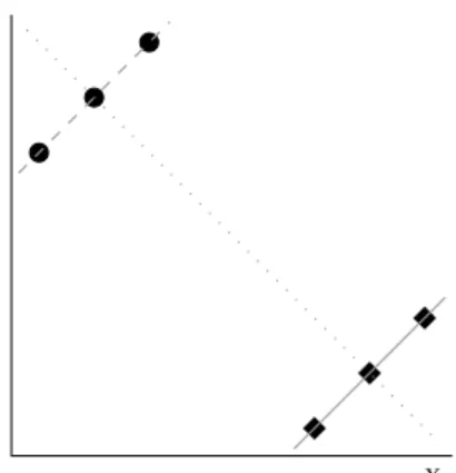
datasetΩ. The simple constructed example from Figure 3.1 illustrates that these two comparisons can lead to very different outcomes.
Suppose that we have a two-dimensional target space, and we are concerned with finding descriptions having a deviating regression line in these two dimensions. Figure 3.1 depicts the target space, and the six records in the example dataset. The dotted grey line is the regression line of the whole dataset, with slope −1. Now suppose that we find the description
3.2. HOW TO DEFINE AN EMM INSTANCE? 25
regression line of GD, with slope 1. The solid grey line is the regression
line of GC
D, also having slope 1. When gauging the exceptionality of a
description solely by the slope of the regression line, we findGD interesting
when compared to Ω, but not at all when compared to GC
D. Of course, the
assessment changes when we include the intercept in the evaluation.
The problem as displayed in Figure 3.1 is underdetermined; we have not enough information to formulate an opinion on whether the subgroup should be deemed interesting. It can therefore not be used to illustrate whether comparing to GC
D or to Ωis preferable; it merely illustrates that a different
choice may lead to a different outcome.
There is not always a clear-cut preferred choice whether to compare toGC D
or to Ω. Sometimes, the real-life problem at hand can point in one di-rection: if we are interested in deviations from a possibly inhomogeneous norm, it makes more sense to compare toΩ, whereas if we are interested in dichotomies, it makes more sense to compare toGCD. On other occasions, a statistically inspired quality measure mayrequire choosing eitherΩorGCD, to prevent violation of mathematical assumptions. Lastly, when the model class is so complicated that learning models from data covered by descrip-tions has a nontrivial computational expense, efficiency might dictate the choice: when comparingndescriptions toΩ, learningn+1models suffices, but when comparing them to GC
D, learning 2n models is required.
The previous two practical considerations supersede any personal prefer-ence that we outline; if the model class choice and quality measure design somehow require comparing to either GC
D orΩ, then that is the way to go.
However, when given the choice, we would consider comparing toΩ prefer-able. After all, Exceptional Model Mining is designed as a Local Pattern Mining task, where we strive to find coherent subsets of the data where something interesting is going on. The goal is to pinpoint many such de-viations of the norm, possibly overlapping, without consideration for the coherence and model parameters occurring in the remainder of the dataset. When we compare the model for a subgroup GD to the model for Ω, we
evaluate a subgroup by comparing its behavior to the behavior for the en-tire dataset. This implies that we strive to find subgroups deviating from the norm. By contrast, when we compare the model for a subgroup GD to
the model forGC
behavior on the complement of the dataset. This implies that we strive to find schisms in the dataset: not necessarily one subgroup deviating from the norm, but rather a partitioning of Ω into two subgroups displaying clearly contrasting behavior. We think this is a very interesting task, but it may not strictly adhere to the goals of Exceptional Model Mining.
3.3
Related Work
Exceptional Model Mining extends a vast body of work, of which this sec-tion contains some highlights. First we discuss the search strategies devel-oped to deal with the exponential search space. Then we look into other local pattern mining tasks, and other extensions of Subgroup Discovery. Finally, we discuss how similar questions arise in other data mining disci-plines, and what distinguishes them from EMM.
3.3.1
Search Strategies for SD/EMM
When striving to find interesting subsets of a dataset, the search space is exponential in the number of records. By restricting the problem to finding interesting subgroups, i.e. subsets with a concise description, the search space remains theoretically exponential in size, but we obtain a handle with which we can tackle the problem. Traditionally [55], this is done by compelling all attributes in the dataset to be nominal. In this case, occasionally exhaustive search is possible, using filters akin to the anti-monotonicity constraints known from frequent itemset mining. When not all attributes are nominal, traditionally there was no other option than to resort to heuristic search.
3.3. RELATED WORK 27
In work dedicated to expanding the description language D available to Subgroup Discoverers, Mampaey et al. introduced an efficient treatment of numeric attributes [76]. The description space is not explored exhaus-tively. Instead, the algorithm finds richer descriptions efficiently, by finding an optimal interval for every numeric attribute, and an optimal value set for every nominal attribute. The efficiency comes from considering only descriptions that lie on a convex hull in ROC space, and evaluating them with a convex quality measure. Hence, the method is only suitable for a target concept that can be properly expressed in ROC space, i.e. traditional SD with a nominal target, and a convex concept of interestingness.
Another problem stemming from the exponential search space is the re-dundancy in a resulting description set. When a description is deemed interesting, small variations will very likely deliver other descriptions that are also quite interesting. Therefore it is not uncommon, especially when there are numeric attributes in the dataset, to find the top of a description chart dominated by many copies of what technically may all be slightly different descriptions, which in practice all indicate the same underlying concept. Van Leeuwen et al. [70] introduced three degrees of subgroup redundancy, and incorporated selection strategies based on these redun-dancies in a beam search algorithm. This results in non-exhaustive, but interestingly different search strategies.
The only work so far on exhaustive Exceptional Model Mining, is Lem-merich et al.’s GP-Growth algorithm [72], which was discussed in detail earlier in this chapter. It can severely reduce the memory requirement and runtime of an EMM instance, but only when a parallel single-pass algo-rithm with sublinear memory requirements exists to compute the model from a given set of records. This can be done for relatively simple model classes, but not for more computationally expensive model classes (cf. Sec-tion 3.1.3).
3.3.2
Similar Local Pattern Mining Tasks
from Subgroup Discovery, include Contrast Set Mining [4], where the goal is to find “conjunctions of attributes and values that differ meaningfully in their distributions across groups”, and Emerging Pattern Mining [21], which strives to find itemsets whose support increases substantially from one dataset to another. One could view the latter task as an amalgamation of two separate Subgroup Discovery runs (one for each dataset), followed by a search for classification rules (where a found subgroup has class1when found on dataset1, and class 2 when found on dataset 2). Kralj Novak et al. provide a framework unifying Contrast Set Mining, Emerging Pattern Mining, and Subgroup Discovery [65].
Giving a full overview of all work related to Subgroup Discovery is beyond the scope of this dissertation; such overviews are available in the literature (for instance: [50]). In the remainder of this section we focus on work related to supervised local pattern mining with a more complex goal.
As the antithesis to Contrast Set Mining, Redescription Mining [39, 91] seeks multiple descriptions of the same subgroups, originally in itemset data. Recent extensions incorporate nominal and numeric data [38].
Umek et al. [109] consider Subgroup Discovery with a multi-dimensional output space. They approach this data by considering the output space first: agglomerative clustering in the output space proposes candidate sub-groups that have records similar in outcomes. Then, a predictive modeling technique is used to test for each identified candidates whether they can be characterized by a description over the input space.
3.3. RELATED WORK 29
3.3.3
Similar Tasks with a Broader Scope
General concepts from EMM, like fitting different models to different parts of the data, or identifying anomalies in a dataset, appear in tasks beyond Local Pattern Mining. In this section we discuss a few such tasks, and how they relate to EMM.
In Outlier Detection, traditionally the goal is to identify records that devi-ate from a general mechanism. Usually there is no desire to find a coherent set of such outliers, which can succinctly be described: identifying non-conforming records is enough. As Outlier Detection becomes more and more mature and sophisticated, we witness more attention towards the un-derlying mechanism making a point an outlier, for instance in recent work by Kriegel et al. [66]. Their method to detect outliers in arbitrarily oriented subspaces of the original attribute space also delivers an explanation with each outlier, consisting of two parts: an error vector, pointing towards the expected position of the outlier, and an outlier score, quantifying the like-liness that this point is an outlier. Searching for the reason for outliers is a step towards bridging the gap with finding coherent deviating subsets as done in EMM, although the approaches differ vastly. Alternatively, Konijn et al. [63] have designed a hybrid method, post-processing regular Outlier Detection results with a Subgroup Discovery run. This enables higher-level analysis of Outlier Detection results.
A similar caveat holds for the well-known Classification And Regression Trees [7], where a nominal or numeric target concept is assigned a differ-ent class or outcome depending on conditions on attributes. While the recursive partitioning given by the tree ensures that every path from the root to a leaf constitutes a coherent, easy to describe subgroup, there is again no explicit search for exceptionalities. A partition that performs well is enough, and if multiple exceptional phenomena that happen to have similar effects on the target are found in the same cell of the partition, the CART algorithm judges this as a good outcome while from the Exceptional Model Mining viewpoint it is not.
As an extension of the regression tree algorithm provided by CART, where the leaves contain numeric values as opposed to the classes found in the leaves of a decision tree, the M5 system [90] produces trees having multi-variate linear regression models in the leaves. Instead of learning a global model for the entire dataset, M5 partitions the dataset by means of the internal nodes of the tree, and learns a local model for each leaf. Essen-tially, the resulting tree can be seen as a piecewise linear regression model. M5 can also be seen as a sibling of Regression Clustering, but with an easy-to-describe partition and a hierarchical clustering. As is the case with CART and Regression Clustering, contrary to EMM the goal of M5 is not to find exceptionalities but to completely partition the data, and the focus is on the overall performance in the target space rather than separation of exceptional phenomena.
3.4. SOFTWARE 31
The work on PCTs has been generalized to concern the general problem of mining on a dataset with structure on the output classes, whether this structure takes the form of dependencies between classes (tree-shaped hi-erarchy, directed acyclic graph) or internal relations between classes (se-quences). A tree ensemble method for such data was proposed by Kocev et al. [61]. Their method is able to give different predictions for parts of the dataset that behave differently from the norm. Contrary to EMM, there is no explicit identification of the deviating subgroup and model.
3.4
Software
In the following chapters, we will introduce model classes and quality mea-sures, and run experiments with the corresponding Exceptional Model Min-ing instances. These experiments are primarily performed with the Cor-tana discovery package [78]: a Java implementation that is an open-source spin-off of the Safarii Data Mining system.
Cortana is not limited to Exceptional Model Mining; it provides multiple supervised Local Pattern Mining tasks. The user can set the task he/she wants Cortana to perform by selecting a target concept. For the simplest target concept, SINGLE_NOMINAL, the user must highlight one nom-inal attribute, and Cortana will perform Subgroup Discovery with that attribute as target. Similarly, for the SINGLE_NUMERIC target concept, one numeric attribute needs singling out, for Cortana to use as numeric target in a Subgroup Discovery run. Several Exceptional Model Mining in-stances are covered by other target concepts: DOUBLE_CORRELATION handles the Correlation model from Chapter 4, the MULTI_LABEL target concept corresponds to the Bayesian network model from Chapter 6, and the DOUBLE_REGRESSION target concept concerns the simple Regres-sion model from Section 7.4. For each target concept, a range of quality measures is available that allow the user to define exactly what sort of ex-ceptional subgroups Cortana should search for. The subgroup validation method we develop in Chapter 8 is also available in Cortana.
[70]), and the user can select one of many strategies for dealing with numeric attributes. Furthermore, conditions can be set on the minimal subgroup size, the minimal subgroup quality, the maximal description length, the maximal number of subgroups to present at the end of the algorithm, and the maximal amount of total time the algorithm spends on the task.
Apart from many more things, Cortana provides a parametrized version of the Beam Search algorithm for Top-q Exceptional Model Mining, as detailed in Algorithm 1. It is available online, at http://datamining.
Chapter 4
Deviating Interactions – Correlation
Model
An Exceptional Model Mining instance strives to find subgroups, for which a particular kind of interaction between multiple target attributes is un-usual, when compared to that same interaction between the same attributes on the entire dataset. Possibly the simplest such interaction is the correla-tion model. In this correlacorrela-tion model, we consider two numeric targets, `1
and`2. Within this model class, we will refer to them as x=`1 andy=`2.
We are interested in their linear association as measured by the correlation coefficient ρ, estimated by the sample correlation coefficient
^
r=
P
xi−¯x yi−y¯
qP
(xi−¯x)2P(yi−y¯)2
where xi denotes the ith observation on x, and ¯x denotes its mean. We let
ρG and ρGC
denote the population coefficients of correlation for Gand GC,
respectively, and let^rG and^rGC
denote their sample estimates.
4.1
Quality Measure
ϕ
scdTo find descriptions with a substantial coverage and deviating correlation coefficient, we develop a statistically-oriented quality measure, based on the test
H0:ρG =ρG
C
against H1 :ρG6=ρG
C
Generally, the sampling distribution of^ris unknown. Ifxandyfollow a bi-variate normal distribution, we can apply the Fisherztransformation
z0 = 1
2ln
1+ ^r 1− ^r
The sampling distribution of z0 is approximately normal [84]. Its standard error is given by
1
√
ξ−3
where ξ is the size of the sample. As a consequence
z∗ = z
0−zC0
q
1 n−3 +
1 nC−3
approximately follows a standard normal distribution under H0. Here z0
and zC0 are the z-scores obtained through the Fisher z transformation for
G and GC, respectively. If both n and nC are greater than 25, then the
normal approximation is quite accurate, and can safely be used to com-pute the p-values. As quality measure ϕscd (acronym for Significance of Correlation Difference) we take 1 minus the computed p-value. Because we have to introduce the normality assumption to be able to compute the
p-values, ϕscd should be viewed as a heuristic measure. Transformation of the original data (for example, taking their logarithm) may make the normality assumption more reasonable.
4.2
Experiments
4.2.1
Datasets
The Windsor Housing dataset [2] concerns 546 houses that were sold in Windsor, Canada in the summer of 1987. The information for each house includes the two attributes of interest, `1 = x = lot_size and `2 =
4.2. EXPERIMENTS 35
Table 4.1: Statistics concerning the datasets used in the Correlation model (this chapter), Classification model (Chapter 5), and alternative Regression model (Section 7.4) experiments. Here, N is the total number of records,
k is the number of descriptive attributes, and m is the number of targets on which the model is fitted.
Dataset Domain N k m
Affymetrix Bioinformatics 63 311 2
Windsor Housing Residential property value 546 10 2
coincides with a higher sales price. The fitted regression function is y =
34136+6.60·x, showing that on average one extra square meter corresponds to a sales price increase of $6.60.
The Affymetrix dataset comes from the domain of bioinformatics. In ge-netics, genes are organised in so-called gene regulatory networks. This means that the expression (its effective activity) of a gene may be influenced by the expression of other genes. Hence, if one gene is regulated by another, one can expect a linear correlation between the associated expression-levels. In many diseases, specifically cancer, this interaction between genes may be disturbed. The Affymetrix dataset shows the expression-levels of 313
genes as measured by an Affymetrix microarray, for 63 patients that suffer from a cancer known as neuroblastoma [64]. Additionally, the dataset con-tains clinical information about the patients, including age, sex, stage of the disease, etc. As targets, we consider the expressions of the two genes
ZHX3 (‘Zinc fingers and homeoboxes 2’) and NAV3 (‘Neuron navigator
3’), showing a slightly positive overall correlation of 0.218.
4.2.2
Experimental Results
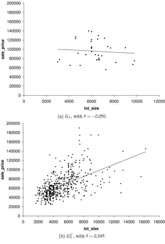
On the Windsor Housing dataset, we run an experiment with ϕscd. As discussed in Section 4.1, in order to be confident about the test results for this quality measure, the coverage of a description has to be over 25. This number was used as minimum support threshold for a run of Cortana using
D1 :drive=1∧rec_room=1∧nbath≥2
This is the group of 35 houses (covering 6.4% of the dataset) that have a driveway, a recreation room and at least two bathrooms. The scatter plots for theD1andDC1 are given in Figure 4.1. The subgroup shows a correlation
of ^rG1 = −0.090 compared to r^GC1 = 0.549 for the remaining 511 houses. A tentative interpretation could be that D1 describes houses in the higher
segments of the market where the price of a house is mostly determined by its location and facilities. The desirable location may provide a natural limit on the lot size, such that this is not a factor in the pricing. Figure 4.1 supports this hypothesis: houses inD1tend to have a higher price ($95, 947
on average, versus $68, 122 on the whole dataset).
In general sales_price and lot_size are positively correlated, but EMM discovers a description with a slightly negative correlation. However, this value is not significantly different from zero: a test of
H0 : ^rG1 =0 against H1 : ^rG1 6=0
yields a p-value of 0.61. The scatter plot confirms our impression that
sales_priceandlot_size are uncorrelated within the description. For pur-poses of interpretation, it is interesting to perform some post-processing. In Table 4.2 we give an overview of the correlations within different de-scriptions whose intersection produces the final result, as given in the last row. It is interesting to see that the conditionnbath ≥2 in itself actually leads to a slight increase in correlation compared to the whole database, but the combination with the presence of a recreation room leads to a sub-stantial drop to ^r = 0.129. When we add the condition that the house should also have a driveway we arrive at the final result with^r= −0.090. Note that adding this last condition only eliminates 3 records (the size of the subgroup goes from 38 to 35) and that the correlation between sales price and lot size in these three records (defined by the condition
4.2. EXPERIMENTS 37 0 20000 40000 60000 80000 100000 120000 140000 160000 180000 200000
0 2000 4000 6000 8000 10000 12000
lot_size s a le _ p ri c e
(a)G1, with^r= −0.090.
0 20000 40000 60000 80000 100000 120000 140000 160000 180000 200000
0 2000 4000 6000 8000 10000 12000 14000 16000 18000
lot_size s a le _ p ri c e
(b)GC
1, with^r=0.549.
Figure 4.1: Windsor Housing - ϕscd: Scatter plot of lot_size and
sales_price for the subgroupG1corresponding to descriptionD1 :drive=
Table 4.2: Descriptions on the housing data, and their sample correlation coefficients and supports.
D ^rGD |G
D|
Whole dataset 0.536 546
nbath≥2 0.564 144
drive=1 0.502 469
rec_room =1 0.375 97
nbath≥2∧drive=1 0.509 128
nbath≥2∧rec_room=1 0.129 38
drive=1∧rec_room =1 0.304 90
nbath≥2∧rec_room=1∧ ¬drive=1 −0.894 3
nbath≥2∧rec_room=1∧drive=1 −0.090 35
4.3
Alternatives
A logical consideration for a quality measure would be the absolute differ-ence of the correlation for the descriptionD and its complement, i.e.
ϕabs(D) =
^rGD − ^rGCD
Unfortunately, this measure does not take into account the coverage of the descriptions, and hence does not do anything to prevent overfitting.
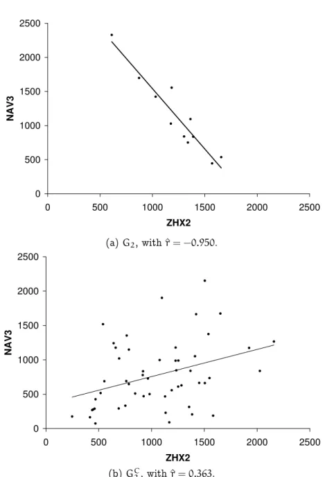
On theAffymetrix dataset, recall that we analyse the correlation between
ZHX3 and NAV3, showing a very slight correlation (^r = 0.218) on the whole dataset. We analyze this dataset in terms of the absolute difference of correlationsϕabs, allowing the use of all remaining attributes (both gene expression and clinical information) for building descriptions. As theϕabs
measure does not have any provisions for promoting larger subgroups, we use a minimum support threshold of10 (15% of the patients). The largest distance (ϕabs(D2) =1.313) was found with the following description
cov-ering 11 records (17.5%) of the dataset
D2:11_band=‘no deletion’∧survival time≤1919∧XP_498569.1≤57
4.3. ALTERNATIVES 39
0 500 1000 1500 2000 2500
0 500 1000 1500 2000 2500
ZHX2
N
A
V
3
(a)G2, with^r= −0.950.
0 500 1000 1500 2000 2500
0 500 1000 1500 2000 2500
ZHX2
N
A
V
3
(b)GC2, with^r=0.363.
Figure 4.2: Affymetrix -ϕabs: Scatter plot of the subgroup corresponding
to description D2 : 11_band = ‘no deletion’∧survival time ≤ 1919∧
and the correlation in the remaining data is ^rGC
2 = 0.363. Note that the description displays a very “stable” behavior: all points are quite close to the regression line, with R2 ≈0.9.
As an improvement ofϕabs, the following quality function weighs the abso-lute difference between the correlations with the entropy function of the split between the description and its complement, as introduced in Sec-tion 3.2.1. Hence, when we find descripSec-tions with ϕabs, but we find their coverage not substantial enough, we can solve this problem by running EMM with the alternative quality measure ϕent, defined as
ϕent(D) =ϕef(D)·
^rG− ^rGC
4.4
Conclusions
In this chapter, we propose to use the correlation between two numeric targets as a measure of exceptionality for descriptions. This is probably the simplest form of target interplay for which Exceptional Model Mining can find deviating descriptions. As such, a domain expert should be able to easily interpret not only a found description, but also the associated model. As we have seen, particularly in discussing description D1 found
on theWindsor Housing dataset, a rationale for a subgroup can relatively easily be given based on the domain-specific interpretation of attributes on which the description is defined. This rationale can be fortified straight-forwardly by inspecting the corresponding sample correlation coefficients. The statistical test, yielding the impression that the targets are uncorre-lated within D1, gives us confidence that the rationale makes sense. Also,