What Cannot Be Computed Locally!

(1)

What Cannot Be Computed Locally!

∗

Fabian Kuhn

Dept. of Computer Science ETH Zurich

8092 Zurich, Switzerland

Thomas Moscibroda

Roger Wattenhofer

ABSTRACT

We give time lower bounds for the distributed approxima-tion of minimum vertex cover (MVC) and related problems such as minimum dominating set (MDS). In k communi-cation rounds, MVC and MDS can only be approximated by factors Ω(nc/k2

/k) and Ω(∆1/k_/k_{) for some constant} _c_, wherenand ∆ denote the number of nodes and the largest degree in the graph. The number of rounds required in order to achieve a constant or even only a polylogarith-mic approximation ratio is at least Ω( logn/log logn) and Ω(log ∆/log log ∆). By a simple reduction, the latter lower bounds also hold for the construction of maximal matchings and maximal independent sets.

Categories and Subject Descriptors

F.2.2 [Analysis of Algorithms and Problem Complex-ity]: Nonnumerical Algorithms and Problems— computa-tions on discrete structures;

G.2.2 [Discrete Mathematics]: Graph Theory—graph al-gorithms;

G.2.2 [Discrete Mathematics]: Graph Theory—network problems

General Terms

Algorithms, Theory

Keywords

approximation hardness, distributed algorithms, dominat-ing set, locality, lower bounds, maximal independent set, maximal matching, vertex cover

∗_{The work presented in this paper was supported (in part)} by the Hasler Stiftung (Berne, Switzerland) and by the Na-tional Competence Center in Research on Mobile Informa-tion and CommunicaInforma-tion Systems (NCCR-MICS), a center supported by the Swiss National Science Foundation under grant number 5005-67322.

Permission to make digital or hard copies of all or part of this work for personal or classroom use is granted without fee provided that copies are not made or distributed for profit or commercial advantage and that copies bear this notice and the full citation on the first page. To copy otherwise, to republish, to post on servers or to redistribute to lists, requires prior specific permission and/or a fee.

1. INTRODUCTION AND

RELATED WORK

What can be computed locally? Naor and Stockmayer [18] raised this for the distributed computing community vital question over a decade ago, and though the price of lo-cality has puzzled researchers ever since, results have been rare [15]. The importance of locality stems from the desire of achieving a global goal based on local information only. This is not only one of the key challenges when developing fast distributed algorithms, but it also improves fault-tolerance and allows detecting illegal global configurations by check-ing local conditions [1]. Recent advances in networkcheck-ing and ever-growing distributed systems drive the need for a thor-ough understanding of locality issues. In the present paper, we study the impact of locality in the classicmessage pass-ing model where the distributed system is modelled as a graph: Nodes represent the processors and two nodes can communicate if and only if they share an edge in the graph. We present lower bounds for several traditional graph theory problems, starting out with minimum vertex cover (MVC). A vertex cover for a graphG= (V, E) is a subset of nodes V0 ⊆V such that, for each edge (u, v) ∈E, at least one of the two incident nodes u, v belongs toV0_{. Finding}

a vertex cover with minimum cardinality is known as the MVC problem.

In local algorithms, nodes are only allowed to communi-cate with their direct neighbors inG. After several rounds of communication they need to come up with a global solution, e.g. a good approximation for MVC. Intuitively MVC could be considered perfectly suited for a local algorithm: A node should be able to decide whether to join the vertex cover by communicating with its neighbors a few times. Very distant nodes seem to be superfluous for this decision. The fact that there is a simple greedy algorithm which approximates MVC within a factor 2 in the global setting, additionally raises hope for an efficient local algorithm.

To our surprise, however, there is no such algorithm. In this paper, we show that inkcommunication rounds, MVC can only be approximated by a factor Ω(nc/k2_/k_{) for a} con-stant c larger than 1/4. This implies a running time of Ω( logn/log logn) in order to achieve a constant or even polylogarithmic approximation ratio. When making the re-sult dependent on the maximum degree ∆ instead of the number of nodesn, the approximation ratio is Ω(∆1/k_/k₎ and the time needed to obtain a polylogarithmic or con-stant approximation is Ω(log ∆/log log ∆). The results for MVC can be extended to minimum dominating set (MDS) and other distributed covering problems. Further, the time

(2)

lower bounds for constant MVC approximations also apply for the construction of maximal matchings and maximal in-dependent sets. Since all lower bounds hold even in the cases of unbounded messages and complete synchrony, the lower bounds are a true consequence of locality limitations, and not merely a side-effect of congestion, asynchrony, or limited message size.

Moreover, some of our lower bounds are almost tight for many cases. In k rounds, MVC can be approximated by a factor O(∆1/k) [10]. In order to obtain a polylogarith-mic approximation, we have to setk= O(log ∆/log log ∆), for a constant approximation, the number of rounds isk= O(log ∆). Hence, for polylogarithmic (and worse) approx-imation ratios, our lower bound is tight whereas for con-stant approximation algorithms, it is tight up to a factor O(log log ∆). For the MDS problem, recent results show that ink rounds, the respective linear program can be ap-proximated up to a factor ∆c/√k_{, whereas for MDS itself} an approximation ratio of ∆c/√k_{ln ∆ can be achieved [9,} 10]. If message size and local computations are unbounded, the MDS LP and MDS can be appoximated up to factors O(n1/k_{) and O(}_n1/k_{ln ∆), respectively [10]. It is easy to} verify that the lower bounds for MDS also holds for the frac-tional LP version. The best known algorithms for maximal matching and maximal independent set need time O(logn) [8, 17].

A pioneering and seminal lower bound by Linial [15] shows that the non-uniform O(log∗n) coloring algorithm by Cole and Vishkin [2] is asymptotically optimal for the ring. This lower bound has been cherished by researchers as a funda-mental advancement in the theory of distributed algorithms. For different models of distributed computation, there is a number of other lower bounds [6, 11], most notably for the problem of constructing a minimum spanning tree (MST) of the network graph [3, 4, 16, 20]. With the exception of [3], the MST lower bounds apply to a model where message size is bounded. In [4], the lower bounds of [16, 20] are extended to approximation algorithms. To the best of our knowledge, it is the only previous lower bound on distributed hardness of approximation.

Linial’s lower bound [15] is based on thedrosophila mela-nogaster of distributed computing, the ring network. For the MVC problem, highly symmetric graphs such as rings often feature a straight-forward solution with constant ap-proximation ratio. In anyδ-regular graph, for example, the algorithm which includes all nodes in the vertex cover is already a 2-approximation for MVC: Each node will cover at mostδedges, the graph hasnδ/2 edges, and therefore at leastn/2 nodes need to be in the minimum vertex cover. On the other extreme, asymmetric graphs often enjoy constant-time algorithms, too. In a tree, choosing all inner nodes yields a 2-approximation. The same trade-off exists for node degrees. If the maximum node degree is low (constant), we can tolerate to choose all nodes, and have by definition a good (constant) approximation. If there are nodes with high degree, the diameter of the graph is small, and a few com-munication rounds suffice to inform all nodes of the entire graph. What we need is a construction of a not too sym-metric and not too asymsym-metric graph with a variety of node degrees! Not many graphs with these “non-properties” are known in distributed computing.

The proof of our lower bounds is based on the timeless in-distinguishability argument [7, 12]. Inkrounds of

commu-nication, a network node can only gather information about nodes which are at most khops away and hence, only this information can be used to determine the computation’s out-come. In particular, we show that after k communication rounds two neighboring nodes see exactly the same graph topology; informally speaking, both neighbors are equally qualified to join the vertex cover. However, in our example graphs, choosing the wrong neighbor will be ruinous.

The remainder of the paper is organized as follows. Sec-tion 2 describes the model of computaSec-tion. The lower bound is constructed in Section 3. In Section 4, we show how our MVC lower bound can be extended to minimum dominating set (MDS), maximal matching (MM), and maximal indepen-dent set (MIS). Section 5 concludes the paper.

2. MODEL

We consider the classicmessage passingmodel, which con-sists of a point-to-point communication network, described by an undirected graph G = (V, E). Nodes correspond to processors and edges represent communication channels be-tween them. In one communication round, each node of the network graph can send an arbitrarily long message to each of its neighbors. Local computations are for free and ini-tially, nodes have no knowledge about the network graph. They only know their own unique identifier.1 Ink commu-nication rounds, a nodevmay collect the IDs and intercon-nections of all nodes up to distancekfromv. Tv,k is defined to be the topology seen byvafter thesekrounds, i.e.Tv,k is the graph induced by thek-neighborhood ofvwhere edges between nodes at exactly distance kare excluded. The la-belling (i.e. the assignment of IDs) of Tv,k is denoted by L(Tv,k).

Because message size is unbounded, the best a deter-ministic algorithm can do in time k, is to collect its k -neighborhood and base its decision on (Tv,k,L(Tv,k)). In other words, a deterministic distributed algorithm can be regarded as a function mapping (Tv,k,L(Tv,k)) to the possi-ble outputs. For randomized algorithms, the outcome ofvis also dependent on the randomness computed by the nodes inTv,k.

The model presented is in accordance with the one used in [15] and textbooks [19]. It is the strongest possible model when proving lower bounds for local computations because it focuses entirely on the locality of distributed problems and abstracts away other issues arising in the design of dis-tributed algorithms (e.g. need for small messages, fast local computations, etc.). This guarantees that our lower bounds are true consequences of locality.

3. LOWER BOUND

We first give an outline of the proof. The basic idea is to construct a graphGk= (V, E), for each positive integerk, which contains a bipartite subgraphSwith node setC0∪C1

and edges inC0×C1 as shown in Figure 1. SetC0 consists

ofn0 nodes each of which hasδ0 neighbors inC1. Each of

then0·δ_δ0

1 nodes inC1hasδ1,δ1> δ0, neighbors inC0. The

goal is to constructGkin such a way that all nodes inv∈S see the same topology Tv,k within distancek. In a globally optimal solution, all edges ofS may be covered by nodes in C1 and hence, no node inC0 needs to join the vertex cover. 1_{Our results hold for any possible ID space including the}

(3)

In a local algorithm, however, the decision of whether or not a node joins the vertex cover depends only on its local view, that is, the pair (Tv,k,L(Tv,k)). We show that because adjacent nodes inSsee the sameTv,k, every algorithm adds a large portion of nodes inC0to its vertex cover in order to

end up with a feasible solution. In other words, we construct a graph in which the symmetry between two adjacent nodes cannot be broken within k communication rounds. This yields suboptimal local decisions and hence, a suboptimal approximation ratio. Throughout the proof, we will useC0

andC1to denote the two sets of the bipartite subgraphS.

Our proof is organized as follows. The structure of Gk is defined in Subsection 3.1. In Subsection 3.2, we show howGk can be constructed without small cycles, ensuring that each node sees a tree within distancek. Subsection 3.3 proves that adjacent nodes inC0andC1have the same view

Tv,k and finally, Subsection 3.4 derives the lower bounds.

3.1 The Cluster Tree

The nodes of graphGk= (V, E) can be grouped into dis-joint sets which are linked to each other as bipartite graphs. We call these disjoint sets of nodesclusters.

We define the structure ofGkusing a directed treeCTk= (C,A) with doubly labelled arcs`:A → × . We refer to CTkas thecluster tree, because each vertexC∈ Crepresents a cluster of nodes inGk. The size of a cluster|C| is the number of nodes the cluster contains. An arca= (C, D)∈ Awith`(a) = (δC, δD) denotes that the clustersC andD are linked as a bipartite graph, such that each nodeu∈C hasδCneighbors inDand each nodev∈DhasδDneighbors inC. It follows that|C| ·δC =|D| ·δD. We call a cluster leaf-clusterif it is adjacent to only one other cluster, and we call itinner-cluster otherwise.

Definition _3.1. _{The cluster tree} _CT_k _{is recursively}

de-fined as follows:

CT1 := (C1,A1), C1 := {C0, C1, C2, C3}

A1 := {(C0, C1),(C0, C2),(C1, C3)}

`(C0, C1) := (δ0, δ1), `(C0, C2) := (δ1, δ2),

`(C1, C3) := (δ0, δ1)

GivenCTk−1, we obtainCTk in two steps:

• For each inner-cluster Ci, add a new leaf-cluster Ci0 with`(Ci, Ci0) := (δk, δk+1).

• For each leaf-cluster Ci of CTk−1 with (Ci0, Ci) ∈ A

and`(Ci0, Ci) = (δp, δp+1), add k−1new leaf-clusters

Cj0 with`(Ci, Cj) := (0 δj, δj+1)forj= 0. . . k, j6=p+1.

Further, we define|C0|=n0 for allCTk.

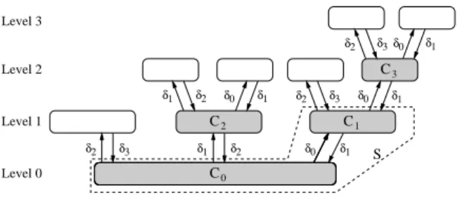
Figure 1 shows CT2. The shaded subgraph corresponds

toCT1. The labels of each arca∈ Aare of the form`(a) =

(δl, δl+1) for somel∈ {0, . . . , k}. Further, setting|C0|=n0

uniquely determines the size of all other clusters. In order to simplify the upcoming study of the cluster tree, we need two additional definitions. Thelevel of a cluster is the distance toC0in the cluster tree (cf. Figure 1). Thedepthof a cluster

C is its distance to the furthest leaf in the subtree rooted at C. Hence, the depth of a cluster plus one equals the height of the subtree corresponding toC. In the example of Figure 1, the depths ofC0,C1,C2, andC3 are 3, 2, 1, and

1, respectively.

1 2

δ δ₃ δ₂ δ₀ δ₁

δ0 δ1 δ₃ δ2 δ0 δ1

δ3 δ2 δ₂ δ0 δ₁ δ₁

δ

Level 0 Level 1 Level 2 Level 3

3 2

C

0

C

S

1

C

Figure 1: Cluster-TreeCT2.

Note thatCTk describes the general structure of Gk, i.e. it defines for each node the number of neighbors in each clus-ter. However,CTk does not specify the actual adjacencies. In the next subsection, we show thatGkcan be constructed so that each node’s view is a tree.

3.2 The Lower Bound Graph

In Subsection 3.3, we will prove that the topologies seen by nodes in C0 and C1 are identical. This task is greatly

simplified if each node’s topology is a tree (rather than a general graph) because we do not have to worry about cycles. The girth of a graphG, denoted byg(G), is the length of the shortest cycle in G. We want to construct Gk with girth at least 2k+ 1 so that ink communication rounds, all nodes see a tree. Given the structural complexity ofGk for largek, constructingGk with large girth is not a trivial task. The solution we present is based on the construction of the graph family D(r, q) as proposed in [13]. For given r and q, D(r, q) defines a bipartite graph with 2qr _nodes and girth g(D(r, q)) ≥r+ 5. In particular, we show that for appropriate r and q, we obtain an instance of Gk by deleting some of the edges of D(r, q). In the following, we introduceD(r, q) up to the level of detail which is necessary to understand our results. For the interested reader, we refer to [13].

For an integerr≥1 and a prime powerq,D(r, q) defines a bipartite graph with node setP∪Land edgesED⊂P×L. The nodes ofP andLare labelled by ther-vectors over the finite field q, i.e.P =L=

r

q. In accordance with [13], we denote a vectorp∈P by (p) and a vectorl∈Lby [l]. The components of (p) and [l] are written as follows (forD(r, q), the vectors are projected onto the firstr coordinates):

(p) = (p1, p1,1, p1,2, p2,1, p2,2, p02,2, p2,3, p3,2, . . .

pi,i, p0i,i, pi,i+1, pi+1,i, . . .) (1) [l] = [l1, l1,1, l1,2, l2,1, l2,2, l02,2, l2,3, l3,2, . . .

li,i, l0i,i, li,i+1, li+1,i, . . .]. (2) Note that the somewhat confusing numbering of the compo-nents of (p) and [l] is chosen in order to simplify the following system of equations. There is an edge between two nodes (p) and [l], exactly if the firstr−1 of the following conditions hold (fori= 2,3, . . .).

l1,1−p1,1 = l1p1

l1,2−p1,2 = l1,1p1

l2,1−p2,1 = l1p1,1

li,i−pi,i = l1pi−1,i (3) l0i,i−p0i,i = li,i−1p1

li,i+1−pi,i+1 = li,ip1

(4)

In [13], it is shown that for odd r ≥ 3, D(r, q) has girth at least r+ 5. Further, if a node u and a coordinate of a neighbor v is fixed, the remaining coordinates of v are uniquely determined. This is concretized in the next lemma.

Lemma _3.2. _{For all} ₍_p₎_∈_P _and_l₁_∈ q, there is exactly one [l] ∈ L such that l1 is the first coordinate of [l] and

such that (p) and [l] are connected by an edge in D(r, q). Analogously, if[l] ∈L and p1 ∈ q are fixed, the neighbor (p)of[l]is uniquely determined.

Proof. _{The first}_r₋_{1 equations of (3) define a linear}

system for the unknown coordinates of [l]. If the equations and variables are written in the given order, the matrix cor-responding to the resulting linear system of equations is a lower triangular matrix with non-zero elements in the diag-onal. Hence, the matrix has full rank and by the basic laws of (finite) fields, the solution is unique. Exactly the same argumentation holds for the second claim of the lemma. We are now ready to construct Gk with large girth. We start with an arbitrary instanceG0

kof the cluster tree which may have the minimum possible girth 4. An elaboration of the construction of G0

k is deferred to Subsection 3.4. For now, we simply assume that G0

k exists. Both Gk and G0k are bipartite graphs with odd-level clusters in one set and even-level clusters in the other. Let m be the number of nodes in the larger of the two partitions ofG0

k. We chooseq to be the smallest prime power greater than or equal tom. In both partitions V1(G0k) and V2(G0k) of G0k, we uniquely label all nodesvwith elementsc(v)∈ q.

As already mentioned,Gkis constructed as a subgraph of D(r, q) for appropriate r andq. We choose q as described above and we setr= 2k−4 such thatg(D(r, q))≥2k+ 1. Let (p) = (p1, . . .) and [l] = [l1, . . .] be two nodes ofD(r, q).

(p) and [l] are connected by an edge in Gk if and only if they are connected inD(r, q) and there is an edge between nodesu∈V1(G0k) andv∈V2(G0k) for whichc(u) =p1 and

c(v) =l1. Finally, nodes without incident edges are removed

fromGk.

Lemma 3.3. The graphGkconstructed as described above is a cluster tree with the same degreesδi as in G0k. Gk has at most2mq2k−5 nodes and girth at least2k+ 1.

Proof. The girth directly follows from the construction; removing edges cannot create cycles.

For the degrees between clusters, consider two neighboring clustersC0

i⊂V1(G0k) andCj0 ⊂V2(G0k) inG0k. InGk, each node is replaced byq2k−5 _{new nodes. The clusters} _C

i and Cj consist of all nodes (p) and [l] which have their first coordinates equal to the labels of the nodes inC0

i and Cj0, respectively. Let each node inC0

i haveδα neighbors in Cj0, and let each node inCj0 haveδβneighbors inCi0. By Lemma 3.2, nodes inCi have δα neighbors in Cj and nodes in Cj haveδβ neighbors inCi, too.

Remark.

In [14], it has been shown thatD(r, q) is discon-nected and consists of at least qbr+24 c isomorphic

compo-nents which the authors callCD(r, q). Clearly, those com-ponents are valid cluster trees as well and we could use one of them for the analysis. As our asymptotic results remain unaffected by this observation, we continue to use Gk as constructed above.

3.3 Equality of Views

In this subsection, we prove that two adjacent nodes in clustersC0 andC1have the sameview, i.e. within distance

k, they see exactly the same topologyTv,k. Consider a node v ∈ Gk. Given that v’s view is a tree, we can derive its view-tree by recursively following all neighbors of v. The proof is largely based on the observation that corresponding subtrees occur in both node’s view-tree.

LetCi andCj be adjacent clusters inCTk connected by `(Ci, Cj) = (δl, δl+1), i.e. each node in Cihas δlneighbors inCj, and each node inCj hasδl+1 neighbors inCi. When

traversing a node’s view-tree, we say that weenter cluster Cj(resp.,Ci) overlinkδl(resp.,δl+1) from clusterCi(resp., Cj). Furthermore, we make the following definitions:

Definition 3.4. The following nomenclature refers to sub-trees in the view-tree of a node in Gk.

• Mi is the subtree seen upon entering clusterC0 over a

linkδi.

• Bi,d,λ is a subtree seen upon entering a cluster C ∈ C \ {C0}over a linkδi, whereC is on levelλand has depthd.

Definition 3.5. When entering subtreeBi,d,λfrom a clus-ter on level λ−1 (λ+ 1), we write B↑

i,d,λ (B

↓

i,d,λ). The predicate ¬ inBi,d,λ¬ denotes that instead ofδi, the label of the link into this subtree isδi−1.

The predicate ¬ is necessary when, after enteringCj from Ci, we immediately return to Ci on link δi. In the view-tree, the edge used to enterCj connects the current subtree to its parent. Thus, this edge is not available anymore and there are onlyδi−1 edges remaining to return toCi. The predicates↑and↓describe from which “direction” a cluster has been entered. As the view-trees of nodes inC0 andC1

have to be absolutely identical for our proof to work, we must not neglect these admittedly tiresome details.

The following example should clarify the various defini-tions. Additionally, you may refer to the example ofG3 in

Figure 3 in the appendix.

Example _3.6. _Consider_G₁_{. Let}_V_C

0 andVC1 denote the

view-trees of nodes inC0 andC1, respectively:

VC0 =B ↑

0,1,1∪B

↑

1,0,1 VC1 =B ↑

0,0,2∪M1

B↑

0,1,1 =B

↑

0,0,2∪M1¬ B0↑,0,2=B

↓,¬

1,1,1

B↑

1,0,1 =M2¬ M1 =B0↑,,1¬,1∪B

↑

1,0,1

· · · ·

We start the proof by giving a set of rules which describe the subtrees seen at a given point in the view-tree. We call these rules derivation rules because they allow us to derive the view-tree of a node by mechanically applying the matching rule for a given subtree.

Lemma 3.7. The following derivation rules hold inGk: Mi=

j=0...k j6=i−1

B↑

j,k−j,1∪ B

↑,¬

i−1,k−i+1,1

B↑

i,d,1=F{i+1}∪D{}∪ Mi¬+1

B↓

i,d,1=F{i−1,k−d+1}∪D{}∪Mk−d+1∪B↑i−,¬1,d−1,2

B↑

(5)

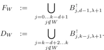
whereF andD are defined as

FW :=

j=0...k−d+1

j /∈W B↑

j,d−1,λ+1

DW :=

j=k−d+2...k j /∈W

B↑

j,k−j,λ+1.

Proof. _{We first show the derivation rule for}_M_{i. It can}

be seen in Example 3.6 that the rule holds fork = 1. For the induction step, we build CTk+1 from CTk as defined in Definition 3.1. M(k) is an inner cluster and therefore, one new clusterBk+1,0,1 is added. The depth of all other

subtrees increases by 1 and M(k+1) := _j₌₀_...k₊₁B↑

j,k−j,1

follows. If we enterM(k+1) over link δi, there will be only δi−1−1 edges left to return to the cluster from which we

had enteredC0. Consequently, the linkδi−1 features the¬

predicate.

The remaining rules follow along the same lines. LetCibe a cluster with entry-linkδi which was first created inCTr, r < k(Note that inCTk,r=k−dholds because each sub-tree increases its depth by one in each “round”). According to the second building rule of Definition 3.1,rnew neighbor-ing clusters (subtrees) are created inCTr+1. More precisely,

a new cluster is created for all entry-linksδ0. . . δr, exceptδi. We call these subtreesfixed-depth subtreesF. If the subtree with rootCi has depthdinCTk, the fixed-depth subtrees have depthd−1. In eachCTr0, r0 ∈ {r+ 2, . . . , k},Ci is an inner-cluster and hence, one new neighboring cluster with entry-linkδr0is created. We call these subtrees

diminishing-depthsubtreesD. InCTk, each of these subtrees has grown to depthk−r0_.

We now turn our attention to the differences between the three rules. They stem from the exceptional treatment of level 1, as well as the predicates ↑ and ↓. In B↑

i,d,1, the

link δi+1 returns to C0, but contains only δi+1−1 edges

in the view-tree. InB↓

i,d,1, we have to consider two special

cases. The first one is the link toC0. For a cluster on level

1 with entry-link (fromC0) i, the equalityk =d+iholds

and therefore, the link toC0 is δk−d+1 and thus, Mk−d+1

follows. Secondly, we writeB↑,¬

i−1,d−1,2, because there is one

edge less leading back to the cluster where we had come from. (Note that since we entered the current cluster from a higher level, the link leading back to where we came from isδi−1, instead ofδi+1). Finally inBi,d,λ↑ , we again have to treat the returning linkδi+1 specially.

Note that the general derivation rule forB↓

i,d,λ is missing as we will not need it for the proof.

Next, we define the notion ofr-equality. Intuitively, if two view-trees arer-equal, they have the same topology within distancer.

Definition _3.8. _Let_V₁₌

i=0...kbiandV2= i=0...kb0i be view-trees;biandb0iare subtrees entered on linkδi. Then, V1andV2arer-equal if all corresponding subtrees are(r−1)

-equal,

V1=rV2 ⇐= bir=−1b0_i, ∀i∈ {0, . . . , k}.

Further, all subtrees are 0-equal: Bi,d,λ =0 B_i0_,d0_,λ0 and

Bi,d,λ=0Mi0 for alli, i0, d, d0, λ, andλ0.

Using the notion of r-equality, it is now easy to define what we actually have to prove. We will show that inGk,

VC0 k

= VC1 holds. This is equivalent to showing that each

node inC0sees exactly the same topology within distancek

as its neighbor inC1. We will now establish several helper

lemmas.

Lemma 3.9. Let β and β0 _{be sets of subtrees, and let}

Vv1 = B ↑

i,d,x∪β and Vv2 = B ↑

i,d,y∪β0 be two view-trees. Then, for allxandy

Vv1 r

=Vv2 ⇐= β r−1

= β0.

Proof. Assume that the roots of the subtree ofVv1 and

Vv2areCiandCj. The subtrees have equal depth and

entry-link and they have thus grown identically. Hence, all paths which do not return to clustersCiandCjmust be identical. Further, consider all paths which, aftershops, return toCi andCj over linkδi+1. After theseshops, they return to the

original cluster and see viewsV0

v1andV 0

v2, differing fromVv1

andVv2 only in the placement of the¬predicate. This does

not affectβandβ0_{and therefore,}

Vv1 r

=Vv2 ⇐=V 0

v1 r−s

= V_v0₂ ∧ β r−=1 β0, s >1.

The same argument can be repeated until r−s = 0 and becauseV0

v1 0

= V_v0₂, the lemma follows.

Lemma _3.10. _Let _β _and _β0 _{be sets of subtrees, and let}

Vv1 = B ↑

i,d,x∪β and Vv2 =B ↑

i,d0_,y∪β0 be two view-trees.

Then, for allxandy, and for allr≤min (d, d0),

Vv1 r

=Vv2 ⇐= β r−1

= β0.

Proof. W.l.o.g, we assumed0 _≤_d_{. In the construction}

process of Gk, the root clusters of Vv1 and Vv2 have been

created in stepsk−dandk−d0, respectively. By Definition 3.1, all subtrees with depthd∗_{< d}0_{have grown identically in}

both views. The remaining subtrees ofVv2 were all created

in stepk−d0+ 1 and have depthd0−1. The corresponding subtrees inVv1have at least the same depth and hence, each

pair of corresponding subtrees are (d0_{−1)-equal. It follows}

that for r ≤min (d, d0_{), the subtrees}_B↑

i,d,xand B

↑

i,d0_,y are

identical within distancer. Using the same argument as in Lemma 3.9 concludes the proof.

2 Τ2 Τ1 Τ0

δ4−1

δ1

δ1 V_C

1

δ4−1

δ1

Τ2

δ3+ +1δ2 δ3+ +1δ2

δ3 δ0−1

3

−1

δ2 δ1

δ0

’ ’ ’

δ

V_C

δ

0

2

Τ1 Τ0

Τ

Figure 2: The view-trees VC0 and VC1 in G3 seen

upon using linkδ1.

Figure 2 shows a part of the view-trees of nodes inC0and

C1 inG3. The figure shows that the subtrees with linksδ0

and δ2 cannot be matched directly to one another because

of the different placement of the−1. It turns out that this inherent difference appears in every step of our theorem. However, the following lemma shows that the subtrees T0

(6)

hence, nodes are unable to distinguish them. It is this crucial property of our cluster tree, which allows us to “move” the¬ predicate between linksδiandδi+2and enables us to derive

the main theorem.

Lemma 3.11. Letβandβ0_{be sets of subtrees and let}_V

v1

andVv2 be defined as

Vv1 = M

¬

i ∪B

↑

i−2,k−i,2∪β

Vv2 = Mi ∪B ↑,¬

i−2,k−i,2∪β0.

Then, for alli∈ {2, . . . , k},

Vv1 k−i

= Vv2 ⇐= β k−i−1

= β0.

Proof. Again, we make use of Lemma 3.7 to show that MiandBi↑−2,k−i,2are (k−i−1)-equal. The claim then follows

from the fact that the two subtrees are not distinguishable and the placement of the¬predicate is irrelevant.

Mi = j=0...k

j6=i−1

B↑

j,k−j,1∪ B

↑,¬

i−1,k−i+1,1

B↑

i−2,k−i,2 =

j=0...i+1

j6=i−1

B↑

j,k−i−1,3∪

j=i+2...k B↑

j,k−j,3

∪ B↓,¬

i−1,k−i+1,1

Forj={0, . . . , i−2, i, . . . , k}, all subtrees are equal accord-ing to Lemmas 3.9 and 3.10. It remains to be shown that B↑

i−1,k−i+1,1

k−i−2 = B↓_i

−1,k−i+1,1. For that purpose, we plug

B↑

i−1,k−i+1,1 and B

↓

i−1,k−i+1,1 into Lemma 3.7 and show

their equality using the derivation rules. Let βbe defined asβ:=F_{i−2,i}∪D{}.

B↑

i−1,k−i+1,1 = F{i}∪D{}∪Mi¬ = B↑

i−2,k−i,2∪Mi¬∪β B↓

i−1,k−i+1,1 = F{i−2,i}∪D{}∪Mi∪Bi↑−,¬2,k−i,2

= B↑,¬

i−2,k−i,2∪Mi∪β

Again, ifMiandB↑i−2,k−i,2 are (k−i−3)-equal, we can move

the¬predicate because the subtrees are indistinguishable. Hence, we have to showMik−=i−3B↑_i₋₂_,k₋_i,₂. In the proof,

we have reduced Vv1 k−i

= Vv2 stepwise to an expression of

diminishing equality conditions, i.e. Vv1

k−i

= Vv2 ⇐= Mi k−i−1

= B_i↑₋₂_,k₋_i,₂

⇐= B↑

i−1,k−i+1,1

k−i−2

= B_i↓₋₁_,k₋_i₊₁_,₁

⇐= Mik−=i−3B_i↑₋₂_,k₋_i,₂.

This process can be continued until either B↑

i−1,k−i+1,1

0

=B_i↓₋₁_,k₋_i₊₁_,₁ or Mi=0B_i↑₋₂_,k₋_i,₂

which is always true.

Finally, we are ready to prove the main theorem.

Theorem 3.12. Consider graphGk. LetVC0 andVC1 be

the view-trees of two adjacent nodes in clustersC0 andC1,

respectively. Then,VC0 k =VC1.

Proof. Initially, each node in C0 sees subtree M∗ and

each node inC1 seesB∗,k,1 (∗denotes that the subtree has

not been entered on any link):

VC0 : M∗=

j=0...k B↑

j,k−j,1

VC1 : B∗,k,1=

j=0...k j6=1

B↑

j,k−j,2∪M1.

It followsVC0 k

=VC1 ⇐= B ↑

1,k−1,1

k−1

= M1 because all other

subtrees are (k−1)-equal by Lemma 3.9. Having reduced VC0

k

=VC1 to B ↑

1,k−1,1

k−1

= M1, we can further reduce it to

M2k−=2B₂↑_,k₋₂_,₁:

M1 =

j=1...k B↑

j,k−j,1∪ B

↑,¬

0,k,1

B↑

1,k−1,1 = B

↑

0,k−2,2∪B

↑

1,k−2,2∪D{}∪ M2¬

k−2 =

Lem. 3.11B

↑,¬

0,k−2,2∪B

↑

1,k−2,2∪D{}∪ M2.

By Lemmas 3.9 and 3.10, all subtree are (k−2)-equal, except B↑

2,k−2,1 andM2.

It seems clear that we can continue to reduceVC0 k =VC1

step by step in the same fashion until we reach 0. For the in-duction step, we assumeVC0

k

=VC1 ⇐= B ↑

r,k−r,1

k−r = Mrfor r < kand proveVC0

k

=VC1 ⇐= B ↑

r+1,k−r−1,1

k−r−1 = Mr+1.

Mr =

j=0...k j6=r−1

B↑

j,k−j,1∪ B

↑,¬

r−1,k−r+1,1

B↑

r,k−r,1 =

j=0...r B↑

j,k−r−1,2∪D{}∪ Mr¬+1

k−r−1 =

Lem. 3.11

j=0...r j6=r−1

B↑

j,k−r−1,2∪B

↑,¬

r−1,k−r−1,2

∪

j=r+2...k B↑

j,k−j,2 ∪ Mr+1.

Apart from Mr+1 (resp,. Br↑+1,k−r−1,1), all subtrees are

(k−r−1)-equal by Lemmas 3.9 and 3.10. SinceMr+1and

B↑

r+1,k−r−1,1 are the only subtrees not being immediately

matched, the induction step follows. For r=k−1, we get VC0

k

= VC1 ⇐= B ↑

k,0,1

0

= Mk, which concludes the proof

becauseB↑

k,0,1

0

=Mk is true.

Remark.

As a side-effect, the proof of Theorem 3.12 has highlighted the fundamental significance of thecritical path

P = (δ1, δ2, . . . , δk) inCTk. After following pathP, the view

of a nodev∈C0 ends up in the leaf-cluster neighboringC0

and sees δi+1 neighbors. Following the same path, a node

v0_∈_C

1ends up inC0and sees i_j₌₀δj−1 neighbors. There is no way to match these views. This inherent inequality is the underlying reason for the wayGkis defined: It must be ensured that the critical path is at leastkhops long.

3.4 Analysis

In this subsection, we derive the lower bounds on the ap-proximation ratio ofk-local MVC algorithms. LetOPT be an optimal solution for MVC and letALG be the solution computed by any algorithm. The main observation is that adjacent nodes in the clustersC0andC1have the same view

(7)

and therefore, every algorithm treats nodes in both of the two clusters the same way. Consequently,ALG contains a significant portion of the nodes ofC0, whereas the optimal

solution covers the edges between C0 and C1 entirely by

nodes inC1.

Lemma _3.13. _{Let ALG be the solution of any distributed}

(randomized) vertex cover algorithm which runs for at most

krounds. When applied to Gkas constructed in Subsection 3.2 in the worst case (in expectation), ALG contains at least half of the nodes ofC0.

Proof. _Let_v₀_∈_C₀_and_v₁_∈_C₁ _{be two arbitrary,}

adja-cent nodes fromC0 and C1. We first prove the lemma for

deterministic algorithms. The decision whether a given node venters the vertex cover depends solely on the topologyTv,k and the labellingL(Tv,k). Assume that the labelling of the graph is chosen uniformly at random. Further, letpA

0 and

pA

1 denote the probabilities thatv0andv1, respectively, end

up in the vertex cover when a deterministic algorithmA op-erates on the randomly chosen labelling. By Theorem 3.12, v0 and v1 see the same topologies, that is, Tv0,k = Tv1,k.

With our choice of labels,v0 andv1 also see the same

dis-tribution on the labellingsL(Tv₀,k) andL(Tv₁,k). Therefore it follows thatpA

0 =pA1.

We have chosenv0 andv1 such that they are neighbors in

Gk. In order to obtain a feasible vertex cover, at least one of the two nodes has to be in it. This impliespA

0 +pA1 ≥1

and thereforepA0 =pA1 ≥1/2. In other words, for all nodes

inC0, the probability to end up in the vertex cover is at

least 1/2. Thus, by the linearity of expectation, at least half of the nodes ofC0 are chosen by algorithm A. Therefore,

for every deterministic algorithm A, there is at least one labelling for which at least half of the nodes ofC0are in the

vertex cover.2

The argument for randomized algorithms is now straight-forward using Yao’s minimax principle. The expected num-ber of nodes chosen by a randomized algorithm cannot be smaller than the expected number of nodes chosen by an op-timal deterministic algorithm for an arbitrarily chosen dis-tribution on the labels.

Lemma 3.13 gives a lower bound on the number of nodes chosen by any k-local MVC algorithm. In particular, we have that E [|ALG|] ≥ |C0|/2 = n0/2. We do not know

OPT, but since the nodes of cluster C0 are not necessary

to obtain a feasible vertex cover, the optimal solution is bounded by|OPT| ≤n−n0. In the following, we define

δi:=δi , ∀i∈ {0, . . . , k+ 1} (4) for some valueδ.

Lemma 3.14. Ifk+ 1< δ, the number of nodes nofGk is

n ≤ n0 1 +

k+ 1 δ−(k+ 1)

.

Proof. _{There are}_n₀ _{nodes in}_C₀_{. By (4), the number}

of nodes per cluster decreases for each additional level by a factorδ. Hence, a cluster on level l contains n0/δl nodes. 2_{In fact, since at most}_|_C

0|such nodes can be in the vertex

cover, for at least 1/3 of the labellings, the number exceeds |C0|/2.

By the definition of CTk, each cluster has at most k+ 1 neighboring clusters on a higher level. Thus, the number of nodesnlon levellis upper bounded by

nl ≤ (k+ 1)l· n0

δl.

Summing up over all levelsland interpreting the sum as a geometric series, we obtain

n ≤ n0·

k+1

i=0

k+ 1

δ

l ≤ n0·

∞

i=0

k+ 1

δ

l

= n0+n0 k+ 1

δ

1 1−k+1

δ = n0 1 + k+ 1

δ−(k+ 1) .

It remains to determine the relationship between δ andn0

such thatGkcan be realized as described in Subsection 3.2. There, the construction of Gk with large girth is based on a smaller instance G0k where girth does not matter. Using (4) (i.e. δi := δi), we can now tie up this loose end and describe how to obtainG0

k. The number of nodes per cluster decreases by a factor δ on each level of CTk. Including C0, CTk consists of k+ 2 levels. The maximum number of neighbors inside a leaf-cluster is δk_{. Hence, we can set} the sizes of the clusters on the outermost level k+ 1 to be δk. This implies that the size of a cluster on level l is δ2k+1−l_{. Particularly, the size of} _C0

0 at level 0 in G0k is n0

0 = δ2k+1. Let Ci and Cj be two adjacent clusters with `(Ci, Cj) = (δi, δi+1). Ci andCj can simply be connected by as many complete bipartite graphsK_δi_,δi+1as necessary.

If we assume thatk+1≤δ/2, we haven≤2n0by Lemma

3.14. Applying the construction of Subsection 3.2, we get n0 ≤n00· hn0i2k−5, where hn0i denotes the smallest prime

power larger than or equal ton0_{, i.e.}_h_n0_i_<₄_n0

0. Putting all

together, we get

n0 ≤ (4n00)2k−4 ≤ 42k−4δ4k

2

. (5)

Theorem 3.15. There are graphsG, such that ink com-munication rounds, every distributed algorithm for the min-imum vertex cover problem on G has approximation ratios at least

Ω

nc/k2 k

and Ω ∆

1/k

k

for some constant c≥1/4, wherenand∆denote the num-ber of nodes and the highest degree inG, respectively.

Proof. _{We can choose} _δ _≥₄−1/(2k)_n1/(4k2)

0 due to

In-equality (5). Finally, using Lemmas 3.13 and 3.14, the ap-proximation ratioαis at least

α ≥ n0/2

n−n0

≥ n0/2·δ/2 n0·(k+ 1)

= δ

4(k+ 1) ≥ (n/2)

1/(4k2₎

41+1/(2k)₍_k_{+ 1)} ∈ Ω

n1/(4k2) k

. The second lower bound follows from ∆ =δk+1_.

(8)

Theorem 3.16. In order to obtain a polylogarithmic or even constant approximation ratio, every distributed algo-rithm for the MVC problem requires at leastΩ

logn

log logn andΩ log ∆

log log ∆

communication rounds.

Proof. We set k =β logn/log logn for an arbitrary constant β > 0. When plugging this into the first lower bound of Theorem 3.15, we get the following approximation ratioα:

α ≥ γn

clog logn β2 logn _· 1

β

log logn logn

whereγ is the hidden constant in the Ω-notation. For the logarithm ofα, we get

logα ≥ clog logn

β2_log_n ·logn−

1

2·log logn−logβ

= c

β2 −

1 2

·log logn−logβ.

and therefore

α ∈ Ω

log(n)

c β2−12

.

By choosing an appropriate β, we can determine the ex-ponent of the above expression. For every polylogarithmic termα(n), there is a constantβsuch that the above expres-sion is at leastα(n) and hence, the first lower bound of the theorem follows.

The second lower bound follows from an analogous com-putation by settingk=βlog ∆/log log ∆.

Remark.

By defining δi :=δi, i∈ {0, . . . , k}and δk+1 :=

δk+1/2(instead ofδk+1), we obtain slightly stronger approx-imation lower bounds of

Ω nc/k2−k

and Ω ∆c0/k−k

. (6)

The bounds of (6) clearly do not suffice to improve the re-sults of Theorem 3.16.

4. REDUCTIONS

Using the lower bound for vertex cover, we can obtain lower bounds for several other classical graph problems. In this section, we give time lower bounds for the construction of maximal matchings and maximal independent sets as well as for the approximation of minimum dominating set.

A maximal matching (MM) of a graphGis a maximal set of edges which do not share common end-points. Hence, a MM is a set of non-adjacent edges ofGsuch that all edges in E(G)\MM have a common end-point with an edge in MM. A maximal independent set (MIS) is a maximal set of non-adjacent nodes, i.e. all nodes not in the MIS are non-adjacent to some node of the MIS. The best known lower bound for the distributed computation of a MM or a MIS is Ω(log∗_n₎

which holds for rings [15]. Based on Theorem 3.16, we get the following stronger lower bounds.

Theorem 4.1. There are graphs G on which every dis-tributed, possibly randomized algorithm requires time

Ω

logn

log logn and Ω

log ∆ log log ∆

to compute a maximal matching. The same lower bounds hold for the construction of maximal independent sets.

Proof. It is well known that the set of all end-points of the edges of a MM form a 2-approximation for MVC. This simple 2-approximation algorithm is commonly attributed to Gavril and Yannakakis. The lower bound for the con-struction of a MM therefore directly follows from Theorem 3.16.

For the MIS problem, consider the line graph L(Gk) of Gk. The nodes of a line graphL(G) ofGare the edges of G. Two nodes inL(G) are connected by an edge whenever the two corresponding edges inGare incident to the same node. The MM problem on a graph Gis equivalent to the MIS problem on L(G). Further, if the real network graph isG,kcommunication rounds onL(G) can be simulated in k+ O(1) communication rounds onG. Therefore, the times tto compute a MIS onL(Gk) andt0 _{to compute a MM on}

Gk can only differ by a constant,t≥t0−O(1). Letn0 and ∆0_{denote the number of nodes and the maximum degree of}

Gk, respectively. The number of nodesn of L(Gk) is less thann02/2, the maximum degree ∆ ofGk is less than 2∆0. Because n0 _{only appears as log}_n0_{, the power of 2 does not}

hurt and the theorem holds (logn= Θ(logn0_)).

We conclude this section by considering the problem of approximating the minimum dominating set (MDS) prob-lem. A dominating setSis a subset of the nodes of a graph G such that all nodes ofG are either inS or they have a neighbor inS. In a non-distributed setting, MDS in equiv-alent to the general minimum set cover problem3 _whereas

MVC is a special case of set cover which can be approxi-mated much better. It is therefore not surprising that in a distributed environment, MDS is strictly harder than MVC, too. In the following, we show that this intuitive fact can be formalized.

Theorem _4.2. _{There are graphs} _G_{, such that in}_k

com-munication rounds, every distributed algorithm for the mini-mum dominating set problem onGhas approximation ratios at least

Ω

nc/k2

k

and Ω ∆

1/k

k

for some constant c, where n and ∆denote the number of nodes and the highest degree inG, respectively.

Proof. We show that every MVC instance can be seen as a MDS instance with the same locality. LetG0_{= (}_V0_{, E}0_{) be}

a graph for which we want to solve MVC. We construct the corresponding dominating set graphG= (V, E) as follows. For every node and for every edge inG0_{, there is a node in}

G. We call nodesvn ∈ V corresponding to nodes v0 ∈ V0 n-nodes, and nodes ve ∈ V corresponding to edges e0 ∈ E0 _e_-nodes_{. Two}_n_{-nodes are connected by an edge if and}

only if they are adjacent in G0. An n-node vn and an e -nodeveare connected exactly if the corresponding node and edge are incident inG0_{. There are no edges between two}_e

-nodes. Clearly, the localities ofG0 andGare the same, i.e. k communication rounds on one of the two graphs can be simulated byk+ O(1) rounds on the other graph. LetCbe a feasible vertex cover for G0. We claim that all nodes of

3_{There exist approximation preserving reductions in both}

(9)

Gcorresponding to nodes inCform a valid dominating set onG. By definition, alle-nodes are covered. The remaining nodes ofG are covered because for a given graph, a valid vertex cover is a valid dominating set as well. Therefore, the optimal dominating set onGis at most as big as the optimal vertex cover onG0_{. There also exists a transformation in the}

other direction. LetDbe a valid dominating set onG. IfD contains ane-node ve, we can replace ve by one of its two neighbors. The size of D remains the same and all three nodes covered (dominated) byveare still covered. By this, we get a dominating set D0 _{which has the same size as}_D

and which consists only ofn-nodes. BecauseD0 _dominates

alle-nodes, the nodes ofG0_{corresponding to}_D0_{form a valid}

vertex cover. Thus, MDS onGis exactly as hard as MVC onG0_{and the theorem follows from Theorem 3.15.}

Corollary _4.3. _{To obtain a polylogarithmic or constant}

approximation ratio for minimum dominating set, there are graphs on which every distributed algorithm needs time

Ω

logn log logn

and Ω log ∆ log log ∆

.

Proof. The corollary is a direct consequence of Theorem 4.2 and the proof of Theorem 3.16.

Remark.

Note that in the above corollary, we give a time lower bound for constant MDS approximation although it has been shown that MDS cannot be approximated better than ln ∆ unless NP ⊆ DTIME(nO(log logn)_{) [5]. Because}

local computation is for free in our model, however, it is theoretically possible to get a constant-factor approximation for MDS.

5. CONCLUSIONS

As distributed systems grow larger, it is becoming increas-ingly vital to design algorithms which do not need to main-tain full information about the network. Unfortunately, with a few notable exceptions [15], there have been almost no hard results, which would have shed light into the theoreti-cal possibilities and limitations of lotheoreti-cality-based approaches. We have shown locality-imposed restrictions on the approx-imability and computability of a number of distributed prob-lems. Comparing with the respective upper bounds, some of our lower bounds are near tight. We hope and believe that the various lower bounds given in the present paper will help to ameliorate this situation.

6. REFERENCES

[1] Y. Afek, S. Kutten, and M. Yung. The Local Detection Paradigm and its Applications to Self-Stabilization. Theoretical Computer Science, 186(1-2):199–229, 1997. [2] R. Cole and U. Vishkin. Deterministic Coin Tossing

with Applications to Optimal Parallel List Ranking. Information and Control, 70(1):32–53, 1986. [3] M. Elkin. A Faster Distributed Protocol for

Constructing a Minimum Spanning Tree. InProc. of the 15thAnnual ACM-SIAM Symposium on Discrete Algorithms (SODA), pages 359–368, 2004.

[4] M. Elkin. Unconditional Lower Bounds on the Time-Approximation Tradeoffs for the Distributed Minimum Spanning Tree Problem. InProc. of the 36th ACM Symposium on Theory of Computing (STOC), 2004.

[5] U. Feige. A Threshold of ln n for Approximating Set Cover.Journal of the ACM (JACM), 45(4):634–652, 1998.

[6] F. Fich and E. Ruppert. Hundreds of impossibility results for distributed computing.Distrib. Comput., 16(2-3):121–163, 2003.

[7] M. J. Fischer, N. A. Lynch, and M. S. Paterson. Impossibility of Distributed Consensus With One Faulty Process.J. ACM, 32(2):374–382, 1985.

[8] A. Israeli and A. Itai. A Fast and Simple Randomized Parallel Algorithm for Maximal Matching.

Information Processing Letters, 22:77–80, 1986. [9] F. Kuhn and R. Wattenhofer. Constant-Time

Distributed Dominating Set Approximation. InProc. of the 22nd_{Annual ACM Symp. on Principles of} Distributed Computing (PODC), pages 25–32, 2003. [10] F. Kuhn and R. Wattenhofer. Distributed

Combinatorial Optimization. Technical Report 426, ETH Zurich, Dept. of Computer Science, 2003. [11] E. Kushilevitz and Y. Mansour. An Ω(Dlog(N/D))

Lower Bound for Broadcast in Radio Networks.SIAM Journal on Computing, 27(3):702–712, June 1998. [12] L. Lamport, R. Shostak, and M. Pease. The Byzantine

Generals Problem.ACM Trans. Program. Lang. Syst., 4(3):382–401, 1982.

[13] F. Lazebnik and V. A. Ustimenko. Explicit

Construction of Graphs with an Arbitrary Large Girth and of Large Size.Discrete Applied Mathematics, 60(1-3):275–284, 1995.

[14] F. Lazebnik, V. A. Ustimenko, and A. J. Woldar. A New Series of Dense Graphs of High Girth.Bulletin of the American Mathematical Society (N.S.),

32(1):73–79, 1995.

[15] N. Linial. Locality in Distributed Graph Algorithms. SIAM Journal on Computing, 21(1):193–201, 1992. [16] Z. Lotker, B. Patt-Shamir, and D. Peleg. Distributed

MST for Constant Diameter Graphs. InProc. of the 20th _{Annual ACM Symposium on Principles of} Distributed Computing (PODC), pages 63–71, 2001. [17] M. Luby. A Simple Parallel Algorithm for the

Maximal Independent Set Problem. SIAM Journal on Computing, 15:1036–1053, 1986.

[18] M. Naor and L. Stockmeyer. What Can Be Computed Locally? InProc. of the 25thAnnual ACM Symp. on Theory of Computing (STOC), pages 184–193, 1993. [19] D. Peleg.Distributed Computing: A Locality-Sensitive

Approach. SIAM, 2000.

[20] D. Peleg and V. Rubinovich. A Near-Tight Lower Bound on the Time Complexity of Distributed Minimum-Weight Spanning Tree Construction.SIAM Journal on Computing, 30(5):1427–1442, 2000.

(10)

APPENDIX

δ₂ δ₁

δ₃ δ₀

δ₀ δ₂

δ₃

δ₃ δ₁ δ₀

δ₀ δ₁

δ₂

δ₂ δ₀

δ₃ δ₁δ₀ δ₃ δ₂ δ₁ δ₀ δ₃ δ₂ δ₀

δ₂ δ₁δ₀ δ₃ δ₂δ₀

δ

δ δ2−1δ1δ0 −1

δ3 δ1 δ0

−1 δ2 δ1−1 2

δ

−1 δ3

0 δ

−1 δ2 δ1−1 2

δ

−1

δ3 δ4−1

3 δ

3

δ δ2δ1−1δ0 1 δ

3

δ δ2−1δ1δ0δ3δ2δ1−1δ0 0

δ −1

δ2

−1 δ4

3 δ

0

δ δ3 δ3δ2δ1−1δ0

0 δ −1

δ1 2

δ 3

δ δ2 δ₁ δ0

1 δ 2 δ −1

δ3 δ2δ1δ0−1

−1 δ3 δ2δ1δ0

−1 δ4

3 δ

0 δ

1 δ

3

δ δ2−1δ1δ0δ3δ2δ1−1δ0 2

δ δ0−1

1 δ 2 δ −1

δ3 δ4−1

3 δ

0

δ δ3 δ3δ2δ1−1δ0

0 δ −1

δ1 2

δ 3

δ δ2 δ₁ δ0

1 δ 2 δ −1

δ3 δ2δ1δ0−1

−1 δ3 δ2δ1δ0

−1 δ4

3

δ δ2−1δ1δ0 −1

3

3 δ1

VC₀

V_C

1

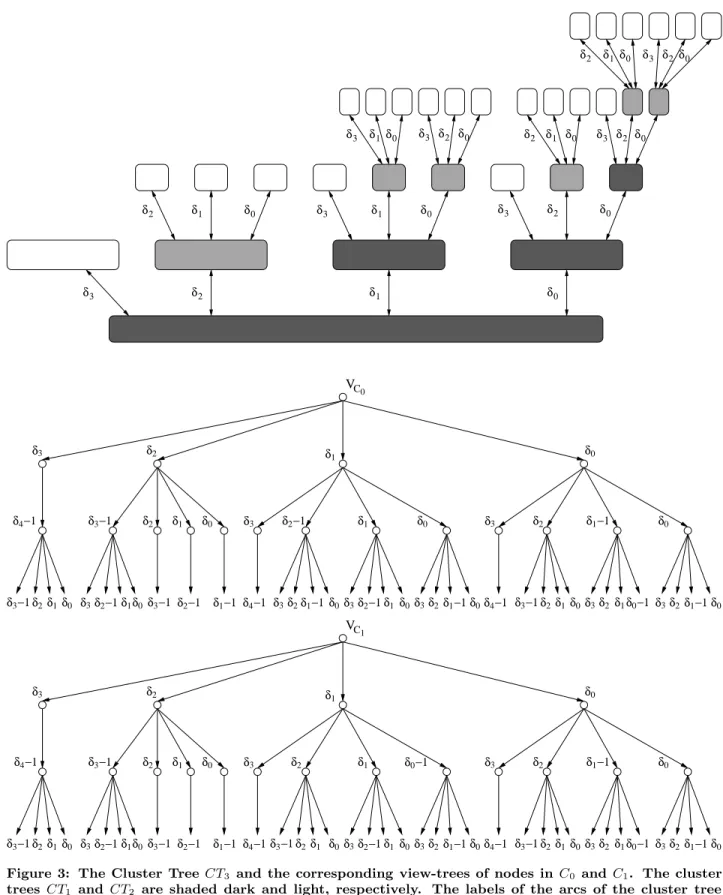
Figure 3: The Cluster TreeCT3 and the corresponding view-trees of nodes in C0 and C1. The cluster

treesCT1 and CT2 are shaded dark and light, respectively. The labels of the arcs of the cluster tree

represent the number of neighbors of nodes of the lower-level cluster in the neighboring higher-level cluster. The labels of the reverse links are omitted. In the view-trees, an arc labelled withδi stands for δi edges, all connecting to identical subtrees.

What Cannot Be Computed Locally!