Comparison of Error Mitigation
Strategies in a Hydrogen Molecule
Quantum Simulation
THESIS
submitted in partial fulfillment of the requirements for the degree of
MASTER OF SCIENCE in
PHYSICS
Author : BSc. X. Bonet-Monroig
Student ID : 1862081
Supervisor : Prof.dr. C.W.J. Beenakker MSc. T.E. O’Brien
2ndcorrector : Dr. V. Cheianov
Comparison of Error Mitigation
Strategies in a Hydrogen Molecule
Quantum Simulation
BSc. X. Bonet-Monroig
Instituut-Lorentz for Theoretical Physics P.O. Box 9506, 2300 RA Leiden, The Netherlands
May 28, 2018
Abstract
Contents
1 Introduction 1
1.1 Quantum computing and quantum chemistry 1 1.1.1 Fundamentals of quantum computing 2 1.1.2 Molecular electronic structure Hamiltonian 4
1.1.3 From quantum chemistry to qubits 5
1.2 Quantum simulations 6
1.2.1 Variational quantum eigensolver 7
1.2.2 Variational algorithms over other methods 9
2 Modeling the hydrogen molecule quantum simulation 11
2.1 The hydrogen molecule 11
2.2 VQE algorithm for the hydrogen molecule 13
2.2.1 Ansatz preparation 14
2.2.2 Measurement 15
2.3 Simulating experimental noise 16
2.3.1 Idling qubits 16
2.3.2 Single-qubit gates 17
2.3.3 Two-qubit gates 17
2.3.4 Measurement 18
2.3.5 Other noise channels 19
2.4 Results 19
3 Error mitigation techniques 21
3.1 Introduction 21
3.2 Parity verification measurement 22
3.3 Quantum subspace expansion 24
3.5 Combining error mitigation techniques 27
3.5.1 Parity verification and QSE/AEM 28
3.5.2 QSE and AEM 28
3.5.3 Parity verification, QSE and AEM 29
3.6 Results 29
4 Conclusions and outlook 35
Chapter
1
Introduction
1.1
Quantum computing and quantum chemistry
The theory of quantum mechanics describes Nature at its smallest scale. Its predictions, which have been extensively proved experimentally, are fundamentally different with respect to classical mechanics. Such a fun-damental difference led Richard Feynman to postulate that if informa-tion could be processed using quantum mechanics, it would lead to an absolutely different theory of information processing [1]. This conjecture opened to door to a new research area, namely quantum computation and information. A quantum computer is the device that carries and manipu-lates quantum information.
Improved fabrication and experimental control of quantum processors have permitted to move from theoretical proposals to practical applica-tions. In this context, quantum chemistry has emerged as one of the most promising fields for which near- and mid-term quantum computers can make an impact. It is expected that these devices will solve the molecular electronic structure problem more accurately than classical computers.
1.1.1
Fundamentals of quantum computing
In a quantum computer the information is stored and processed in a fun-damentally different way than its classical counter-part. The basic unit of a quantum computer is a quantum bit, or qubit, as opposed to a classical bit. The key difference between the bit and the qubit is that the former can only store either a 0 or a 1, whereas the latter can be both 0 and 1 simulta-neously. Therefore, the state of a qubit is described as a linear combination of 0 and 1 as:
|ψi =α|0i+β|1i, (1.1)
where α,β are complex numbers which give the probability of mea-suring (0,1). As the total probability of the state can not be larger than 1, it follows that |α|2+|β|2 = 1. The information is hence stored in a two-dimensional complex vector space. The states |0i and |1i form an orthonormal basis such a vector space, commonly referred as the compu-tational basis. This description extends naturally to a representation of N qubits on aC2via the tensor product.
In order to manipulate the state of a qubit, we need to apply quantum operations. A quantum operation ˆU transforms the state of a qubit from
|ψito|ψ˜isuch that:
|ψ˜i =α˜ |0i+β˜|1i. (1.2)
A transformation of this form requires the operation to be a 2×2 matrix acting on the qubit vector space. Moreover, the fact that |α˜|2+β˜
2
= 1
implies that the operation must be a unitary,UU† = I. A unitary matrix is therefore the quantum counter-part to a “gate” on a classical computer.
Finally, the information stored in a quantum computer must be extracted by measuring the state of the qubit. In quantum mechanics, such a process is describe by Born’s rule: the output of an observable ˆOon the state|ψiis equal to one of the eigenvaluesλiof ˆO
ˆ
1.1 Quantum computing and quantum chemistry 3
with probability
P(λi) =|hλi|ψi|2. (1.4)
When a qubit is measured in a quantum computer, there are only two possible outputs, namely 0 or 1. Based on Born’s rule, the observable of a qubit must necessarily be a matrix with two different eigenvalues. In a quantum computer such observables are the so-called Pauli matrices. In the computational basis, the Pauli matrices{X, Y, Z}take the following form:
X =
0 1 1 0
; Y=
0 −i
i 0
; Z =
1 0
0 −1
The fact that all these three matrices have the same eigenvalues allows us to use any of them as a basis to readout a qubit. Because theZPauli ma-trix is diagonal in the computational basis, it is generally used to measure the qubits. Measurement in the X or Y basis is performed by pre-rotations. On individual qubits, the Pauli operators anti-commute,
{X,Y} ={X,Z} ={Y,Z} =0, (1.5)
but acting on separate tensor factors commute:
[A⊗ I,I ⊗B] =0, (1.6)
for anyA,B =X,Y,Z.
1.1.2
Molecular electronic structure Hamiltonian
The molecular electronic structure Hamiltonian describes the interaction between electrons and nuclei in a Coulomb potential [3]. The dynamics of a system are represented by the position of the electronsri and the po-sition, mass and charge of the nucleiRi, Mi, Zi. The molecular structure Hamiltonian in the first-quantization formalism is given by:
H=−
∑
i
∇2
Ri 2Mi −
∑
i∇2
ri 2 −
∑
i,jZi
Ri−rj
+
∑
i,j>i
ZiZj
Ri−Rj
+
∑
i,j>i 1
ri−rj
.
(1.7)
Within the realm of quantum chemistry, this Hamiltonian is of central interest because almost all properties of the dynamics of a molecule are determined by its eigenstates.
For example, a chemical reaction occurs when the system evolves from one to another stable chemical structure. The energy difference between two stable configurations determine the kinetics of the reaction [4]. Mathe-matically, this is expressed in equation 1.7 by the evolution of the electrons with respect to each other and the nuclei. Those configurations that mini-mize the energy are the most likely to be part of the reaction mechanism. For this reason, accurate calculations of the ground and some excited state energies of this Hamiltonian are important to understand complex chem-ical reaction processes.
Classical computational methods have been extensively used to solve a wide range of electronic structures problems, from molecules to materials. However, for a system with hundred correlated electrons, the accuracy of these techniques no longer allows one to make reliable predictions. The reason is that the number of bits required to store all the information is
∼2100, exceeding the capabilities of the best supercomputers. In contrast, a quantum computer will be able to store the information in a superpo-sition state which will drastically reduce the resources to simulate such problems.
1.1 Quantum computing and quantum chemistry 5
qubits required to simulate quantum systems which exceed the capabili-ties of the best classical computers. Large molecules or strongly correlated materials are amongst the most studied problems in the field [4–8]. For instance, Reiher et al. [4] studied the open problem of biological nitrogen fixation. They predicted that a qualitatively valid result would require
∼104−106physical qubits and a computational time of the order of days including quantum error correction. A recent work by Babbush et al. [8] used a clever choice of the molecular basis to express the molecular struc-ture Hamiltonian, which reduced the required quantum resources. They proposed jellium as a model to study in near-term quantum device includ-ing error mitigation methods instead of costly quantum error correction codes.
1.1.3
From quantum chemistry to qubits
In order to solve the molecular electronic structure Hamiltonian (eq. 1.7) on a quantum computer, we must express it in terms of qubits. Previ-ous works have directly mapped eq. 1.7 onto a quantum computer [6]. However, in this work we use the second quantization formalism before mapping the Hamiltonian onto qubits. We follow the description given in reference [7] to express the molecular structure Hamiltonian in the second quantization formalism.
The first step to transform eq. 1.7 is to take the Born-Oppenheimer ap-proximation, assuming that the motion of the electrons is much faster than the motion of the nuclei. The latter can, therefore, be treated as a classical point charge. Next, a basis to represent the wave-function of the elec-tronsφi(ri,si)is chosen with a defined positionriand spinsifor each elec-tron. The position and momentum of the electrons are then expressed in terms of the annihilation and creation operators (ai, a†i), which obey the fermionic anti-commutation relations:
{ai,a†j} =aiaj†+a†jai =δi,j,
{ai,a†i} ={aj,a†j} =0. (1.8)
H =
∑
pq
hpqa†paq+1
2pqrs
∑
hpqrsa†
pa†qaras, (1.9)
where the coefficientshpq andhpqrs are calculated from:
hpq =
Z
drdsφ∗p(r,s)
h∇2
r 2 −
∑
iZi
|Ri−r|
i
φq(r,s), (1.10)
hpqrs =
Z
dr1ds1dr2ds2
φ∗p(r1,s1)φq∗(r2,s2)φs(r1,s1)φr(r2,s2)
|r1−r2|
. (1.11)
The potential advantage of a quantum computer over its classical counter-part in simulating molecular structure problems comes from the fact that spin-orbitals can be identified with qubits. This is because a spin-orbital contributes a 2-dimensional Hilbert space tensor factor, which is precisely what a qubit does. Although some theoretical requirements exist for the realization of a qubit [9], in principle any quantum mechanical two-level system can be used as a one.
A qubit is described in terms of Pauli matrices which follow the com-mutation relations previously given in equation 1.6. Hence, a natural way to simulate a Hamiltonian in a quantum computer is in terms of such operators. Mapping the molecular structure Hamiltonian from its anti-commuting fermionic operators (a,a†) onto a qubits is a non-trivial task.
There exist different ways in which this mapping can be done, namely the Jordan-Wigner and the Bravyi-Kitaev transformations. Both provide a recipe to write the anti-commuting fermionic operators as a linear combi-nation of Pauli matrices such that the anti-commutation relations are pre-served.
1.2
Quantum simulations
1.2 Quantum simulations 7
described by Seth Lloyd in [10], a quantum simulation consists of repro-ducing the dynamics of a quantum system by another quantum system. The requirement for such a calculation is that the interactions of the quan-tum system must be controllable experimentally. In other words, we must have the ability to apply quantum gates to reproduce the problem under investigation.
Recent methods that combine quantum and classical resources have emerged as an optimization of classical and quantum computation. In this hybrid quantum-classical paradigm, the computational effort is split between quan-tum and classical resources. A quanquan-tum computer performs those tasks that are more efficient or even impossible to do in a classical computer. In the same way, a classical computer runs those processes which a quantum computer finds difficult.
1.2.1
Variational quantum eigensolver
In the context of quantum-classical algorithms, the variational quantum eigensolver (VQE) [11, 12] has emerged as a candidate to use in the next generation of quantum hardware.
The VQE algorithm can be outlined in the following steps [12]:
1. Prepare a quantum state, ψ(~θ)
E
= U(~θ)
~0
E
, depending on a set of
parameters~θ. These parameters must be experimentally adjustable in the quantum hardware.
2. Measure the energyE(~θ) :=
D
ψ(~θ)
H
ψ(~θ)
E
of the state.
3. MinimizeE(~θ)as a function of the parameters~θwith a classical rou-tine.
The variational principle is used to approximate the expectation value of an observable given a trial wave-function
ψ(~θ)
E
E(~θ)≥E0. (1.12)
This implies that the classical minimization routine can only push our en-ergy closer to the ground state enen-ergy.
Some fundamental limitations of the variational methods must be taken into account while designing a VQE experiment. First, the ansatzes are problem-dependent. They are required to have sufficient overlap with the ground state eigenvector|ψ0i, such that the optimization of the
parame-ters gets close to the exact solution. Unless
ψ(~θ)
E
= |ψ0ifor some~θ, the
minimum energyE(~θ) will be strictly larger thanE0. Moreover, covering
the entire Hilbert space with
ψ(~θ)
E
requires an exponentially large
num-ber of parameters~θ. Therefore, the computation time of the optimization routine might become extremely large [13].
Nevertheless, the fact that quantum resources are used in the VQE al-gorithm allows one to prepare ansatz which cannot be, in principle, com-puted in a classical computer. In particular, trial states which are parametrized by the action of a unitary matrix on a state, emerge naturally in a quantum computer and might not have any classical correspondence [14]. The abil-ity to construct such states opens a window to explore problems for which classical methods ado not achieve reliable results.
The VQE algorithm has been successfully applied experimentally in the context of quantum simulations of small molecules [11, 15, 16]. These ex-periments use very different choices of ansatz: for instance, O’Malley et al. [15] used the unitary coupled cluster (UCC) ansatz taken from the cou-pled cluster method in computational chemistry. By contrast, Kandala et al. [16] designed an ansatz based on the capabilities of their quantum de-vices: choosing the more accurate quantum gates that could be performed experimentally.
1.2 Quantum simulations 9
1.2.2
Variational algorithms over other methods
The following quote by Frank Wilczek encompasses the long-time belief that quantum computers will help to solve problems in research areas that will directly impact society:
“In the 21st century quantum computers will do for molecular design what classical computers did for aircraft design in the 20th century”
To fulfill these expectations, we must show that the upcoming quantum algorithms match or improve upon the best classical algorithm. Quantum chemistry and correlated electron problems have been largely studied us-ingab initiomethods developed in computational chemistry. Solving those problems with quantum algorithms allows their capabilities to be bench-marked against state-of-the-art computational methods. Some of the most important computational chemistry techniques are:
• Hartree-Fock: This method describes the motion of single electrons in the field of the nuclei and the average field of the other elec-trons [17]. However it does not account for electron correlations, thus it does not provide good results for strongly correlated systems.
• Density functional theory (DFT): In DFT, the problem of interact-ing electrons in an static potential is reduced to a problem of non-interacting electrons moving in an effective potential [18]. Although DFT has been applied to study large systems of electrons with great success, the results become inaccurate when the problem involves strong correlations. Furthermore, DFT does not allow for the estima-tion or bounding of the errors.
• Coupled Cluster (CC): In this method the excitation operator that promotes electrons from occupied to excited orbitals is exponenti-ated. The CC ansatzes are prepared by the action of this exponential operator acting on the vacuum [19].
• Other methods: Monte-carlo and Density-matrix renormalization group are the most advanced classical methods. They show good results for strongly correlated systems but are computationally in-tensive if one aims to get small errors for systems with 50 electrons and beyond.
• Quantum phase estimation algorithm (QPE): The QPE algorithm is designed to find the phase that a unitary transformation adds to its eigenstates. It is expected that for large enough steps of the al-gorithm the result converges to the true eigenvalue of the unitary. However, the existing theoretical proposals require quantum error correction for large systems with the current error rates [7].
Chapter
2
Modeling the hydrogen molecule
quantum simulation
2.1
The hydrogen molecule
The hydrogen molecule (H2) is a good first toy model for studying
quan-tum algorithms applied to quanquan-tum chemistry. Despite its simplicity, it provides a playground to experimentally test and benchmark the capabil-ities of small quantum devices.
If we are to simulate the hydrogen molecule in a quantum computer, it is necessary to find the number of qubits required to experimentally do so. In quantum chemistry, qubits are identified with spin-orbitals. Hence, for H2, where the 2 ls spin-orbitals form a minimal basis, the number of qubits
is four.
From equation 1.9, one observes that the Hamiltonian can be divided into one- and two-electron parts:
H=
4
∑
p,q=1hpqa†paq+ 1 2
4
∑
pqrs=1hpqrsa†pa†qaras =H(1)+H(2), (2.1)
bond length (d) between the two hydrogen atoms. The minimal basis to represent the hydrogen molecule requires to add the 4 spin-orbitals in the previous expressions.
Following the calculation by Whitfield et al. [7], the one-electron Hamil-tonian is of the form:
H(1) =h
11a†1a1+h22a†2a2+h33a3†a3+h44a†4a4, (2.2)
and the two-electron Hamiltonian:
H(2) =h
1221a†1a†2a2a1+h3443a†3a4†a4a3+h1441a†1a4†a4a1+
h2332a†2a†3a3a2+ (h1331−h1313)a†1a†3a3a1+ (h2442−h2424)a†2a4†a4a2+
h1423(a†1a†4a2a3+a†3a†2a4a1) +h1243(a†1a2†a4a3+a†3a†2a4a1)+
h1423(a†1a†4a2a3−a†3a†2a4a1) +h1243(a1†a†2a4a3−a†3a†2a4a1).
(2.3)
Next, one expresses the above equation in terms of operators which can be measured on a quantum computer, this is, mapping the anti-commuting fermionic operators onto Pauli operators. In this work, we use the Bravyi-Kitaev (B-K) transformation [20], which results in the following form at each bond length (d) [21]:
H= f0I+f1Z0+ f2Z1+ f3Z2+f1Z0Z1
+f4Z0Z2+ f5Z1Z3+ f6X0Z1X2+f6Y0Z1Y2
+f7Z0Z1Z2+ f4Z0Z2Z3+ f3Z1Z2Z3
+f6X0Z1X2Z3+ f6Y0Z1Y2Z3+ f7Z0Z1Z2Z3.
(2.4)
Here, Ii, Xi, Yi, Zi are the Pauli matrices acting on the i-th qubit, and XiZj = Xi⊗Zj refers to the tensor product of the operators. The coef-ficients fi are calculated from equation 1.10 and 1.11. We use the open-source package for quantum chemistry on a quantum computer Open-Fermion [22] to calculate these coefficients.
2.2 VQE algorithm for the hydrogen molecule 13
it is possible to solve the problem in a single simultaneous eigenspace of Z1 and Z3. As the true ground eigenstate of H2 is guaranteed to have
non-zero overlap with the Hartree-Fock state|0000i, it must lie in the+1 eigenspace ofZ1andZ3. By using this symmetry we can effectively reduce
the full Hamiltonian from four to two qubits, leaving:
H =g0I+g1Z0+g2Z1+g3Z0Z1+g4X0X1+g5Y0Y1, (2.5)
where the coefficientsgiare calculated from the two- and four-body in-tegrals (1.10,1.11) and depend upon the bond length.
2.2
VQE algorithm for the hydrogen molecule
In the rest of this section, we present a VQE algorithm in a hybrid quantum-classical architecture for the hydrogen molecule, and detail the measure-ment protocol.
The VQE algorithm can be split into two parts, one involving quan-tum resources and one with a classical computer. In the quanquan-tum part, a small quantum computer is used to prepare and measure a quantum state. We differentiate between the state preparation and the measurement, al-though experimentally they act as one. The data processing is done in the classical section: the coefficients giare calculated, the expectation value is obtained as a weighted sum of individual Hamiltonian terms 2.5, and a minimization routine is launched to suggest new parameters. This is re-peated until the parameters converge to a set of values which represent the approximated ground state energy,E(~θ).
At the same time that we are searching for interesting problems to solve on a quantum computer, we are also interested in understanding which trial states can be efficiently prepared in small quantum devices. For in-stance, it is known that the Hilbert space of N-qubits can be parametrized with p=2N+1−2.
Hamiltonian). If one aims to use a VQE algorithm to simulate large sys-tems, taken advantage of the symmetries will be important to minimize the computational resources required for it.
2.2.1
Ansatz preparation
A general 2-qubit system requires p = 23−2 = 6 variables to param-eterize its Hilbert space. The hydrogen molecule Hamiltonian (2.5) con-tains only real values, hence half of the parameters are needed to reach its ground state. We can fix one more parameter by enforcing that the ground state energy of the hydrogen molecule lies in the single-excitation mani-fold. With all of the above, we find that only two parameters are needed in our algorithm.
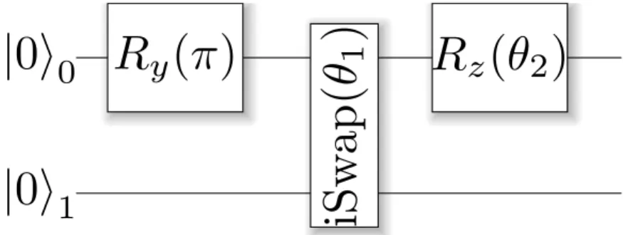
The circuit that prepares the state is given in figure 2.1. In order to pre-pare the state in the single-excitation manifold, we apply a single-qubit ro-tationRy(π). Qubits are entangled with a parametrized two-qubitiSwap(θ1)
gate [23]. Finally, a parametrized single-qubit rotation Rz(θ2), that
ac-counts for any imaginary terms of the Hamiltonian, is applied. Although this circuit prepares a trial state that can be used for any Hamiltonian with real and imaginary values, for the hydrogen molecule problem, which has only real entries, the parametrized Z-rotation is unnecessary to obtain its ground state. Nonetheless, we leave it as a free parameter to observe its experimental behaviour.
|
0
i
0
R
y
(
π
)
|
0
i
1
iSw
ap(
θ
1
)
R
z
(
θ
2
)
Figure 2.1: State preparation circuit parametrized by anglesθ1 &θ2. Qubits are
initialized in the|00istate because its experimental preparation is simple.
Each term of the two-qubit Hamiltonian is measured by preparing the state with the same parametersθ1,θ2. When the energy expectation value
2.2 VQE algorithm for the hydrogen molecule 15
This optimization is repeated until the energy converges to a minimum at~θminAt this point,
ψ(~θmin) E
represents the best estimate of the ground state wave-function. This is repeated for different bond lengths until the dissociation curve is clearly defined. We make use of the Nelder-Mead optimization method through the open source python software SciPy [24, 25].
2.2.2
Measurement
Previously in the text, we have described how to extract the information in a quantum computer. We have mentioned that the state of a qubit is obtained by measuring the Z observable, and also that only partial in-formation of it can be recovered. Therefore, multiple repetitions of the measurement are needed to statistically recover the qubit state.
MeasuringI, Z0, Z1, Z0Z1 is trivial because they are diagonal in the
Z-basis. Furthermore, the fact that all of them commute with each other allow us to use the same single-shot measurements for obtaining their expectation values. By contrast, measuring X0X1 and Y0Y1 requires
pre-rotating the qubit. This allows us to put the qubit in the X or Y basis before reading it out. The extended measurement circuit for these observables is shown in figure 2.2.
From the repeated single-shots, the density matrix of the state is recon-structed and the operators measured as:
ˆ
O
=tr[Oˆρ]. (2.6)
The expectation value of the Hamiltonian is then obtained from the in-dividual expectation values as:
hHi =g0hIi+g1hZ0i+g2hZ1i+g3hZ0Z1i+g4hX0X1i+g5hY0Y1i.
|
ψ
i
0
R
α
(
π
2
)
|
ψ
i
1
R
α
(
π
2
)
Figure 2.2: Measurement circuit for X0X1 & Y0Y1. Here, α = Y,X labels the
rotation to be applied.
2.3
Simulating experimental noise
In this section, we outline the underlying error model of our numerical cal-culations. They have been performed using the quantumsim density ma-trix simulator package [26]. This software allows us to introduce a noise model to describe the qubit architecture imperfections. We use the noise model described by O’Brien et al. [27] for the superconducting transmon qubit architecture [28, 29].
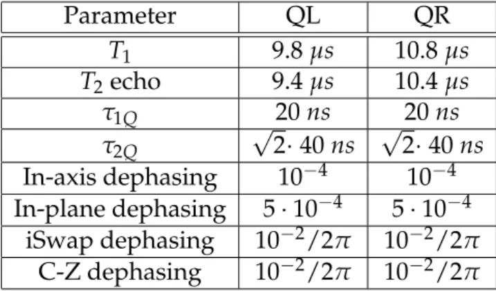
One of the goals of this project is to predict the performance of an ex-isting superconducting qubit device. We have chosen parameters to best model this device within the capabilities of quantumsim (see table 2.1).
Superconducting qubits are prone to errors due to qubit relaxation and dephasing (T1, T2), as well as imprecisions of control hardware (e.g. angle
dephasing) and readout infidelity. The values of T1and T2 have been
ex-perimentally obtained, whilst the rest of the parameters are taken from the literature and internal experimental results.
2.3.1
Idling qubits
When a qubit in the state|1i is idling for a time t it has a probability p1
2.3 Simulating experimental noise 17
probabilities depend on the qubit relaxation and dephasing timeT1,Tφas:
p1=exp
− t
T1
,
pφ =exp
− t Tφ , (2.8)
whereTφ is related to the experimental valuesT1, T2as:
1 T2
= 1
Tφ
+ 1
2T1
. (2.9)
2.3.2
Single-qubit gates
Single-qubit gates are modeled as an instantaneous gate sandwiched by idling gates of time t = τ1Q
2 . In this way, it is possible to separate errors
due to qubit decoherence from those related to hardware control imper-fections.
The instantaneous Ry rotation gate is modeled with an additional de-polarizing noise which corresponds to a shrink towards the origin of the Bloch sphere. The size of this errors is paxis along the y-axis and pplane in the x,z-plane. On the other hand, the instantaneous Rz rotation will only suffer from an over-rotation of the axis (1−paxis).
2.3.3
Two-qubit gates
The model for qubit gates is the same as the single-qubit model; two-qubit gates are applied instantaneously, and sandwiched between two idling gates of time t = τ2Q
2 . In general, quantumsim allows one to
in-dependently set the one- and two-qubit gate times. In our simulations we have set the time to τ2Q = 2
√
2τ1Q, provided by experimental collabora-tors.
the understanding of underlying physical error mechanisms. In our algo-rithm, we use two of these gates with different noise models [23].
1. iSwap: The gate is used to prepare the trial state in its parametrized version. Experimentally this is performed by holding the system for a timeτ(θ)in the|01i ↔ |10iavoided crossing such that the excita-tions are exchanged between the qubits (process matrix given in app. A.). The imperfection on the application of the angle is accounted for by including a small incoherent error in the angle value.
2. CNOT: Experimentally this gate is decomposed in two single-qubit gates and two-qubit C-Z gate (detailed in app. A). The C-Z gate is performed by holding the system for a timeτ2Q at the avoided cross-ing|11i ↔ |02i. The state|01iacquires a phase which is multiple of 2π , whilst the state|11i picks up a phase which is an odd multiple ofπ, as required. Inaccuracies on the phase acquisition are modeled with a small incoherent deviation from the expected phase value. The dephasing parameter is taken from the supplementary material of reference [27].
2.3.4
Measurement
The implementation of the measurement process in our simulations largely differs from the physical realization. Instead of reconstructing the density matrix of the system from single measurements, we extract it from quan-tumsim without collapsing the state. The expectation values are calculated as in equation 2.6. This is justified because the error in measurement can be canceled by careful tomography using linear inversion or maximum likelihood estimation techniques, with one exception: sampling noise.
2.4 Results 19
Table 2.1:Values used in the simulations.
Parameter QL QR
T1 9.8µs 10.8µs
T2echo 9.4µs 10.4µs
τ1Q 20ns 20ns
τ2Q
√
2·40ns √2·40ns In-axis dephasing 10−4 10−4 In-plane dephasing 5·10−4 5·10−4
iSwap dephasing 10−2/2π 10−2/2π C-Z dephasing 10−2/2π 10−2/2π
2.3.5
Other noise channels
Even though the quantumsim package has a very accurate error model, there are noise sources that are not yet incorporated which could have significant effects on the experiment.
First of all, a more thorough noise model is needed for the two-qubit gates, including leakage effects. Leakage occurs when the qubit gets ex-cited out of the two lowest energy levels. The C-Z gate is very sensitive to this effect since the qubit is moved close to the|02istate and there is a non-zero probability to tunnel to it.
Another unmodeled source of noise is qubit-qubit flux cross-talk, and microwave cross-talk. When a qubit is manipulated, neighboring qubits might interfere with it, reducing the fidelity of the process.
2.4
Results
0.5 1.0 1.5 2.0 2.5 Bond distance (Angstroms)
−1.2
−1.0
−0.8
−0.6
−0.4
−0.2 0.0 0.2
Energy
(Hartree)
Noisless qubits Noisy qubits Exact ground energy 0.5 1.0 1.5 2.0 2.5
Bond distance (Angstroms) 10−2
∆Energy
(Hartree) Error in energy Chemical accuracy
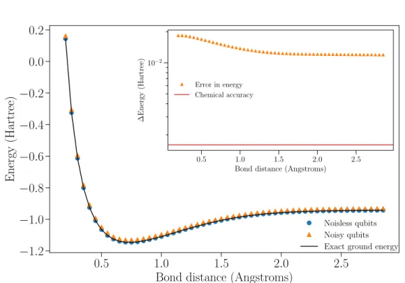
Figure 2.3: Exact dissociation curve (solid black), solution of the VQE algorithm
for noiseless (blue dots) and noisy (orange triangles) qubits. Inset: Deviation from the exact solution under noise effects and chemical accuracy line (solid red).
We first compute the numerical calculation under the ideal scenario of a noiseless device. As expected, the exact solution fully overlaps with the simulation of the experiment (blue dots in figure 2.3). The result is a confirmation that, under ideal conditions, it is possible to calculate the ground state energy of the hydrogen molecule via quantum simulations with 2 qubits. Moreover, it confirms that the code works correctly.
Figure 2.3 additionally shows the simulation result in the presence of experimental noise (orange triangles). The inset of the figure shows the error in energy of the noisy curve with respect to the exact solution (black solid line). As a visual reference, we also include the chemical accuracy threshold (red line).
We conclude that with the available device a quantum simulation ofH2
Chapter
3
Error mitigation techniques
3.1
Introduction
In the previous chapter, we have shown that small calculations on cur-rent quantum hardware are insufficient to make predictions. For instance, a VQE quantum simulation of a molecule with 50 orbitals will require a circuit of length ∼ 10 µs, reaching the limits of our experimental device. Assuming an error probability ofp=5·10−2every 1µs, the estimate error of such a simulation is:
p0=1−(1−p)t0 =1−(1−0.05)10 ∼5·10−1. (3.1)
This result shows that the current technology will not be sufficient to run large calculations. While it is expected that error rates will be reduced in upcoming generations of quantum technology, we do not expect these to be sufficiently reduced for accurate quantum simulations without addi-tional strategies to correct or mitigate remaining errors.
with error rates of 0.1%.
An alternative solution for near-term quantum computers are the so-called error mitigation techniques. They use extra information accessible about the system to reach more accurate results. Error reduction methods represent an intermediate method towards accurate solutions without, or with minimal, QEC .
In this chapter, we apply three error mitigation strategies to a hydrogen molecule quantum simulation to study their performance. We introduce a new technique that we call ‘parity verification’, and apply to other pre-vious developed technique: quantum subspace expansion [31] and active error minimization [32, 33]. The goal is to estimate the error reduction of these strategies for our device. Moreover, we aim to investigate their combination with the idea of reaching chemical accuracy for theH2
disso-ciation curve.
3.2
Parity verification measurement
Given a physical system described by a Hamiltonian H and a conserved quantityC, if
[H,C] =0, (3.2)
we may simultaneously measure H and C. This can be used to verify that the prepared state lies in the subspace in which the desired solution is contained. Experimentally, one will disregard the outputs in which C signals an error.
By enforcing physical symmetries, it is possible to reduce noise due to the interaction between the environment and the quantum computer, also known as incoherent noise. The reason is that the effect of the noise on the state often puts it out of the correct eigenspace of C. By disregarding the measurement, we prevent the error to enter into the final result. We expect this technique to be especially effective because incoherent noise represents the main source of errors on superconducting qubits.
In the hydrogen molecule problem, there exists a conserved quantity that can be used to signal errors. The operator Z0Z1, which contains
3.2 Parity verification measurement 23
|
ψ
i
0
R
α
(
π
2
)
|
ψ
i
1
R
α
(
π
2
)
R
α
(-
π
2
)
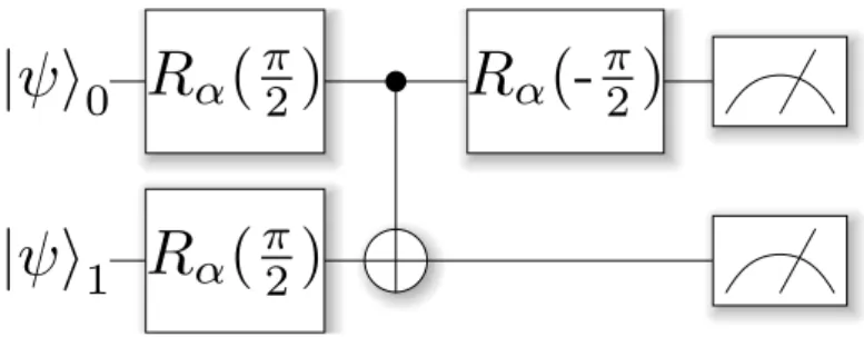
Figure 3.1: Parity verification measurement circuit for X0X1 &Y0Y1. Here,α =
Y,Xlabels the rotation to be applied.
single-excitation manifold and, thus has odd parity. Therefore, it is pos-sible to measure the energy and the parity and disregard those measure-ments that do not satisfy the correct parity. Note that a change in the parity of a state comes from a qubit flipping from the excited to the ground state. A bit-flip error like this occurs when a qubit relaxes, hence we expect to fully mitigate theT1noise channel.
In chapter two, we have described how the individual expectation val-ues are calculated from single-shot measurements, as well as the expecta-tion value of the Hamiltonian. Again, I, Z0, Z1 & Z0Z1 can be obtained
from the same set of measurements. The parity is calculated from the single-shot valuesa =0, 1 orb =0, 1 of each qubit as:
P = (−1)a+b, (3.3)
ifP 6=−1, the measurement is disregarded.
By contrast, measuringZZalong with XXorYY requires an extension of the circuit. It is sufficient to use a single circuit becauseZZ·XX =YY. The extended measurement circuit is shown in figure 3.1. In this circuit, the parity is encoded in the top qubit, whereas the bottom one gets the information of the state. When the top qubit returns a 0, the measurement is disregarded becauseP =1.
3.3
Quantum subspace expansion
McClean et al. [31] developed the quantum subspace expansion (QSE) method to approximate excited states of a Hamiltonian from a ground state wave-function obtained with a quantum computer. The wave-function
|ψ0ibecomes the reference state to explore the spectrum of the system by
extending the Hilbert space with excitations from it. Therefore, the first excited manifold will be found by acting with a single operator on each qubit. The second will be reached by applying excitation to two qubits, and similarly for larger systems.
Mathematically, this will translate into a construction of a new set of vectors|φii, such that:
|φii = Ai|ψ0i, (3.4)
where Ai are the excitations from the reference state. These vectors are then used as a basis to extend the problem HamiltonianHas:
˜
Hi,j =
φj
H |φii =hψ0|A†jHAi|ψ0i. (3.5)
Finally, the excited states are calculated by solving the generalized eigen-value problem of the new Hamiltonian ˜H:
˜
H |λi=λC|λi, (3.6)
where C is the overlap matrix, given by:
Ci,j =
φj
φi
=hψ0|A†jAi|ψ0i (3.7)
In the same paper [31], it is shown that the ground state energy given by the ˜His a more accurate solution than that resulting from|ψ0ialone. The
3.4 Active error minimization 25
The application of QSE as a mitigation strategy requires a careful selec-tion of the set of operators Ai to extend the problem because the number of measurements required grows polynomially with the number of opera-tors. Moreover, prior to the start of the experimental run, one must know which extra measurements are required in the expansion.
In this work, we apply the linear response (LR) expansion, also de-scribed in reference [31], on the two-qubit H2 Hamiltonian (eq. 2.5). The
set of operators in this expansion is given by:
Ai ={I I,ZI,IZ,XI,IX,YI,IY}. (3.8)
The application of these operators on equation 2.5 leads to a 7-dimensional effective Hamiltonian ˜H. In addition to the previous expectation values, ˜H
also depends onhXYiandhYXi. If we are to combine QSE with the parity verification method another measurement circuit is needed. It takes the same form of figure 3.1, with different rotation in each qubit.
In our simulations, QSE is computed as a post-processing step after the optimal set of angles have been obtained from a numerical minimization of the initial circuit. These angles define approximate the lowest eigen-state of the Hamiltonian|ψ0iwhich is necessary to calculate the additional
expectation values. Once all the terms have been measured, the effective Hamiltonian and overlap matrices are computed. Finally, the eigenvalues of these matrices are calculated and its lowest eigenvalue becomes the new energy expectation value.
It is important to mention that a first demonstration of this method to H2 has recently been performed [34]. However, QSE has not been tested
together with other mitigation techniques. We aim to show that it is pos-sible to combine QSE with other methods to reduce the final error in the energy estimate.
3.4
Active error minimization
more accurate solution of the expectation value of a problem Hamiltonian
Hby running experiments with higher error rates.
At the heart of AEM lies the idea that the energy calculated from a noisy quantum computer differs from the true value as:
˜
H
(e) =hHi+ea1+e2a2+e3a3+O(e4), (3.9)
where ˜
H
represents the expectation value ofhHiat a noise levele andak are constants of the noise model. Therefore,e can be accurately calculated as one makes the experiment progressively worse. The error-free expecta-tion value can be obtained from a polynomial extrapolaexpecta-tion ate→0.
Although AEM is an interesting idea to reduce the errors in a compu-tation, its experimental implementation remains unclear. For instance, finding an experimental knob that can be controlled to increase the errors seems a challenging task. Moreover, in the case that one or more of those knobs can be found, they need to be linked to a noise source. Finally, we will not expect that detuning a single parameter will leave the other noise channels static, hence not affecting the final expectation value.
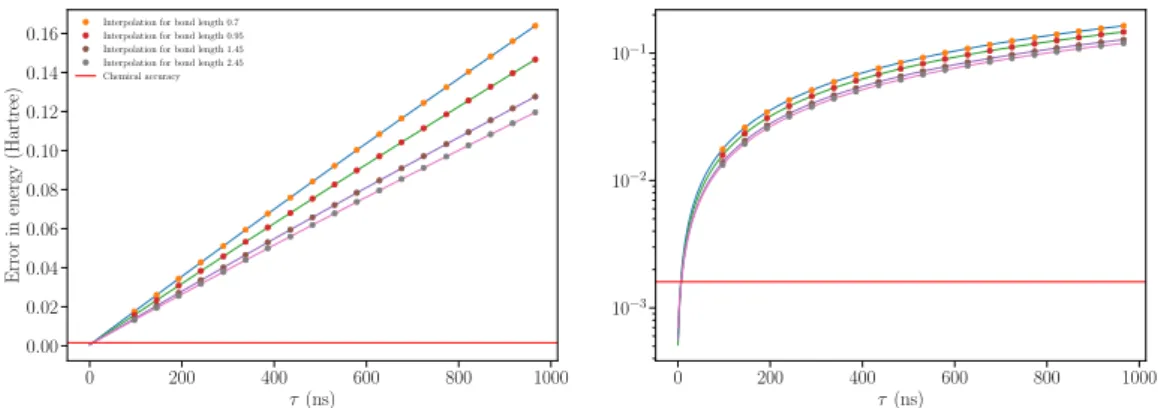
Nonetheless, we simulate the performance of AEM in our existing de-vice. As discussed in section 2.3, this work focuses on cQED transmon qubits which are known to be coherence-limited. The largest sources of error are due to T1 and T2 decay during the experiment. One would
ex-pect that as the circuit time increases, so does the error in the energy be-cause the qubits are longer exposed to decoherence. For this reason, circuit length (τ) can be used as an error parameter in equation 3.9.
In our simulations, τ is tuned by increasing the time of all single- and two-qubit gates. Based on the error model described in section 2.3, this translates into longer idling gates that expose the qubits to more errors due to decoherence. It turns out that this can be realized in our experimental set-up by adding waiting times between the gates.
3.5 Combining error mitigation techniques 27
0 200 400 600 800 1000
τ(ns) 0.00
0.02 0.04 0.06 0.08 0.10 0.12 0.14 0.16
Error
in
energy
(Hartree)
Interpolation for bond length 0.7 Interpolation for bond length 0.95 Interpolation for bond length 1.45 Interpolation for bond length 2.45 Chemical accuracy
0 200 400 600 800 1000
τ(ns) 10−3
10−2
10−1
Figure 3.2: Example of active error minimization for different bond lengths. The
dots are the energy calculated from the VQE experiment at differentτ, the solid
line is the least-square fitting of the energies. Both left and right panels show the same data.
The optimal angles at each point are used to compute the energy of a longer circuits. Experimentally, the computational time needed to do so is approximately one day. Each dissociation curve currently requires 1.5 hours repeated for 19 circuit lengths. In total, we estimate an experimental time of 10 days to implement AEM . Optimizing this is a key target for future research.
Nonetheless, we aim to predict the performance in our existing device, for a simulation of 54 bond distances and 19 circuit lengths. Extrapolation curves for different distances are shown in figure 3.2, in linear (left) and logarithmic (right) scales. The error-free ground state energy is computed from a third order polynomial fit of the minimum energy calculated at differentτ.
3.5
Combining error mitigation techniques
3.5.1
Parity verification and QSE/AEM
The parity verification circuit together with either QSE or AEM is obtained in the same way as for the initial circuit. The ground state energy is com-puted from a numerical optimization of~θwith the parity verification strat-egy.
Next, if we want to overlay this solution with QSE, the optimal angles
~θminmust be fed into the post-processing stage to calculate the additional
terms, compute the matrices and get the lowest eigenvalue of the extended Hamiltonian as the new energy estimate.
In a similar way as before, AEM uses~θmin computed from the parity
verification measurement as previously described.
3.5.2
QSE and AEM
The application of QSE and AEM is done by feeding~θminof the initial
cir-cuit into the QSE data processing. The energy at a given circir-cuit length is obtained from the QSE lowest eigenvalue. By extracting the energy esti-mate from QSE at different circuit lengths, we are able to apply the AEM extrapolation.
While simulating the output of these combinations, we encountered that the lowest eigenvalue goes below the exact solution of the hydrogen molecule. As discussed in the first chapter, the variational principle en-suresE(~θmin)≤E0. Hence, the result obtained does not have any physical
value as it no longer corresponds to our problem Hamiltonian. Further-more, at some bond distances the generalized eigenvalue problem can not be solved because the overlap matrixCcan be made non-positive by nu-merical error.
3.6 Results 29
3.5.3
Parity verification, QSE and AEM
As a final goal of this work, we simulate the combination of the three meth-ods, aiming to push the error of the dissociation curve significantly below the chemical accuracy (CA) threshold.
The implementation requires us to obtain the optimized angles~θmin
from the parity verification measurement. Such angles are then used to calculate the estimate energy from the QSE protocol. This becomes the ground state energy at a given circuit length. The final energy estimate is obtained by repeating this for several circuit lengths, and getting the error-free energy from the AEM protocol.
3.6
Results
In the rest of this chapter, we show the results of the application of the error mitigation techniques to the hydrogen molecule quantum simulation.
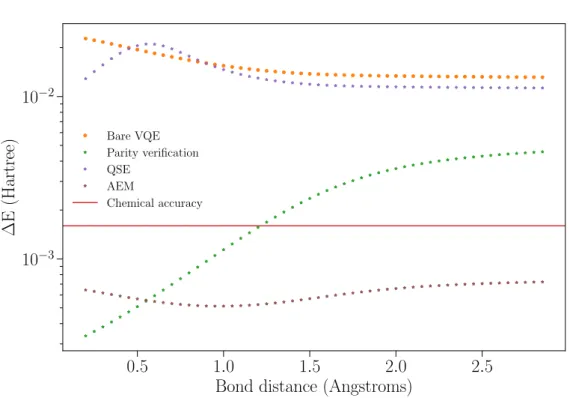
In figure 3.3, we present the error with respect to the exact dissociation curve of a single mitigation technique. The orange dots represent the noisy experiment without error reduction.
From this plot, one already notices that QSE (purple stars) does not provide a significant improvement over the initial result. Furthermore, around R = 0.5 ˚A the error shows a kink that goes above the bare VQE experiment. This is unexpected because one would assume that the low-est eigenvalue of the extended Hamiltonian will be smaller of equal to the reference ground state. A possible explanation is that the additional ex-pectation values calculated from the optimal angles are more noisy than QSE is capable of correcting. However, a more rigorous study is required to understand the possibilities of QSE as a noise cancellation protocol.
mainly caused by the T1 channel, or bit-flips. By verifying the parity, we
are signaling these bit-flips, and thus we are able to eliminate them.
By contrast, at large distances bit-flips are not the only errors disturbing the computation. While we can correct the remaining T1-related errors,
we are largely affected by dephasing due to T2 decay. The reason is that
larger bond lengths require more entanglement between the qubits, thus exposing the system to such noise channels. As proof, in figure 3.4 we show the expectation values of the individual terms of the two-qubit hy-drogen Hamiltonian. Here, one can see that the hXXi = hYYi ∼ 0 for short distances, whilehZIi and hIZi are at their maximum value. When the distance between hydrogen atoms gets larger,hZIi,hIZitend to 0, but
hXXi = hYYi ' −1. Hence, more entanglement is required to accurately measure these expectation values.
The last curve on figure 3.3 (brown stars) shows the error in the energy from the AEM protocol, as described previously. This is approximately the error in our calculation in the absence of decoherence. By only applying AEM in our experiment, we reduce the error from the initial experiment by an order of magnitude, putting the simulation below CA for the entire dissociation curve. The reason for AEM to give such an improvement is that transmon qubits are coherence-limited, thus the time to implement a circuit is the main noise channel.
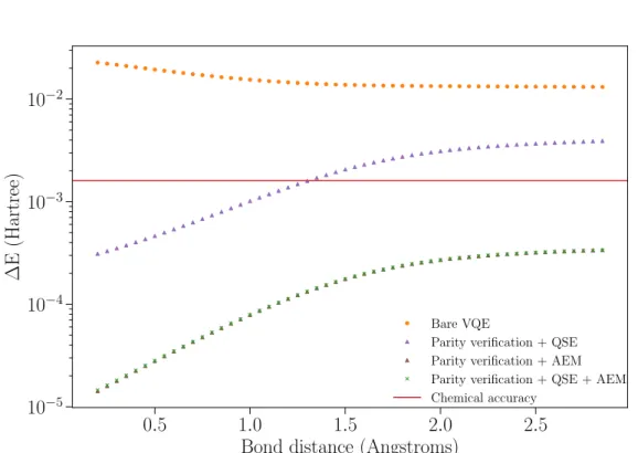
We continue by presenting the combination of two techniques in fig-ure 3.5 (purple and brown triangles). As previously discussed in this chap-ter, the combination of QSE and AEM have not been successful, and we do not include it in the figure.
By looking at the curve of PV and QSE (purple triangles) one notices that the correction is similar to the one given by PV alone. Again, at large bond distances dephasing is the dominant error channel and neither PV nor QSE are able to mitigate it. This simulation also suggests that PV and QSE mitigate similar noise channels.
3.6 Results 31
0.5 1.0 1.5 2.0 2.5 Bond distance (Angstroms)
10−3 10−2
∆E
(Hartree)
Bare VQE Parity verification QSE
AEM
Chemical accuracy
Figure 3.3:Comparison of one mitigation technique with respect to the bare VQE
experiment.
0.5 1.0 1.5 2.0 2.5 Bond distance (Angstroms)
−1.00
−0.75
−0.50
−0.25 0.00 0.25 0.50 0.75 1.00
Exp
ectation
value
hIIi hZIi hIZi hZZi hXXi hY Yi
0.5 1.0 1.5 2.0 2.5 Bond distance (Angstroms)
10−5
10−4 10−3 10−2
∆E
(Hartree)
Bare VQE
Parity verification + QSE Parity verification + AEM Parity verification + QSE + AEM Chemical accuracy
Figure 3.5: Energy error without mitigation and with two and three mitigation
3.6 Results 33
Finally, in figure 3.5 we show the result of combining the three mitiga-tion strategies (green crosses). We observe that the curve fully overlaps with the one of PV and AEM . This shows that QSE no longer suppresses any errors, and only parity verification and AEM are able to mitigate them.
The results seen previously suggest two relevant considerations to be made when planning VQE experiments:
1. Stacking several layers of mitigation does not guarantee a more ac-curate result.
Chapter
4
Conclusions and outlook
In this thesis we have modeled a quantum simulation experiment for the hydrogen molecule using a VQE algorithm to compare three error mitiga-tion techniques. We have used a density-matrix quantum simulator that allows us to introduce a realistic error model based on the current state-of-the-art quantum hardware. Moreover, we have developed a new strategy to signal and eliminate errors that violate physical restrictions of the prob-lem under study. We have further explored existing noise suppression schemes, and analyzed two of them: quantum subspace expansion and active error minimization.
Two main results have been obtained from this work. Firstly, we have estimated the performance of the VQE experiment on an existing device. We have shown that in the absence of error mitigation, it is not possi-ble to achieve a reliapossi-ble result on the dissociation curve of the hydrogen molecule. Secondly, we have explored the capabilities of the same ex-periment in combination with three error mitigation strategies. We have shown that near-term quantum devices can provide accurate solutions without requiring full quantum error correction.
and other quantum algorithms by applying existing, or newly developed error mitigation schemes.
Acknowledgments
I would like to start by thanking Carlo Beenakker and Tom O’Brien for considering me as the suitable candidate for this project, although I was a constant bother at their lectures. I would like to emphasize that Tom has been an incredible supervisor from whom I learned almost everything I know about research, and also has become a very good friend.
Since my very first day at the Nanophysics group, I felt very welcomed and I rapidly became an active member of it. It is an honor, and a priv-ilege, to work with such an extraordinary and smart group of people. I am very grateful to everyone of them: Paul, Nicandro, Maxim, Mar-cello, Lizzy, Yaroslav, Nikolay, Cameron, Slava, Michal, Mark, Jimmy and Marco. Thank you all for never refusing to answer my questions, and for tolerating my “peculiar” vision of life (and death).
I must not forget to include everyone at the Instituut-Lorentz that have helped me, one way or another. In particular, I am very grateful to our secretaries Fran and Manon because without them nothing would be as easy as it is.
Furthermore, I would like to express my gratitude to Leo DiCarlo and his lab for showing and teaching me the beauty of quantum mechanics in action. Brian, Niels, Adriaan, Ramiro, Malay and all the others, thank you all for making me part of what you are trying to achieve.
Appendix
A
Matrix representation of gates
Here we show the matrix representation of the gate set used throughout the text.
Pauli rotations
Rx(θ) =
cosθ
2
isinθ
2
isinθ
2
cosθ
2
(A.1)
Ry(θ) =
cosθ
2
sinθ
2
−sinθ
2
cosθ
2
(A.2)
Rz(θ) =
cosθ
2
+isinθ
2
0
0 cosθ
2
+isinθ
2
(A.3)
Specific Pauli rotations
Rxπ 2
= √1
Ryπ 2
= √1
2
1 1
−1 1
(A.5)
Ry(π) =
0 1
−1 0
(A.6)
Two-qubit Gates
iSwap(θ) =
1 0 0 0
0 cosθ isinθ 0 0 isinθ cosθ 0
0 0 0 1
(A.7) CNOT =
1 0 0 0 0 1 0 0 0 0 0 1 0 0 1 0
(A.8)
In a real experiment a CNOT gate is decomposed as:
CNOT = [I⊗Ry(−π
2)]·CZ·[I⊗Ry( π
2)] (A.9)
Where the new matrices take the following form:
I⊗Ry(−π
2) = 1 √ 2
1 −1 0 0
1 1 0 0
0 0 1 −1
0 0 1 1
(A.10)
I⊗Ry(π
2) = 1 √ 2
1 1 0 0
−1 1 0 0
0 0 1 1
0 0 −1 1
41
CZ =
1 0 0 0 0 1 0 0 0 0 1 0 0 0 0 −1
Bibliography
[1] R. P. Feynman, Simulating physics with computers, International Jour-nal of Theoretical Physics21(1982).
[2] M. Nielsen and I. Chuang, Quantum computation and quantum infor-mation, Cambridge University press, Cambridge, UK, 2001.
[3] T. Helgaker, P. Jorgensen, and J. Olsen, Molecular Electronic Structure Theory, Wiley, New York, 2002.
[4] M. Reiher et al.,Elucidating reaction mechanisms on quantum computers, Proceedings of the National Academy of Sciences114, 7555 (2017).
[5] A. Aspuru-Guzik, A. Dutoi, P. Love, and M. Head-Gordon,Simulated quantum computation of molecular energies, Science309(2005).
[6] I. Kassal et al.,Polynomial-time quantum algorithms for the simulation of chemical dynanmics, PNAS105(2008).
[7] J. D. Whitfield, J. Biamonte, and A. Aspuru-Guzik, Simulation of electronic structure Hamiltonians using quantum computers, Molecular Physics , 735 (2010).
[8] R. Babbush et al., Low depth quantum simulation of electronic structure, arXiv:1706.00023v3 [quant-ph] (2018).
[9] D. DiVincenzo, The physical implementation of quantum computation, arXiv:0002077 [quant-ph] (2000).
[11] A. Peruzzo et al.,A variational eigenvalue solver on a photonic quantum processor, Nature Communications (2014).
[12] J. R. McClean, J. Romero, R. Babush, and A. Aspuru-Guzik,The the-ory of variational hybrid quantum-classical algorithms, New Journal of Physics (2016).
[13] N. Moll et al., Quantum optimization using variational algorithms on near-terms quantum devices, arXiv:1710.01022 [quant-ph] (2017).
[14] Y. Shen et al., Quantum implementation of Unitary Couple Cluster for simulating molecular electronic structure, Phys. Rev. A (2017).
[15] P. J. J. O’Malley et al., Scalable Quantum Simulation of Molecular Ener-gies, Phys. Rev. X6, 031007(13) (2016).
[16] A. Kandala et al.,Hardware-efficient variational quantum eigensolver for small molecules and quantum magnets, Nature6, 242 (2017).
[17] F. Neese et al.,Advanced aspects of ab initio theoretical optical spectroscopy of transition metal complexes: Multiplets, spin-orbit coupling and reso-nance Raman intensities, Coordination Chemistry Reviews 251, 288 (2007).
[18] P. Hohenberg and W. Kohn,Inhomogeneous electron gas, Phys. Rev.136 3B, B864 (1965).
[19] D. Lyakh et al., Multireference nature of chemistry: The coupled cluster view, Chem. Rev.112, 182 (2012).
[20] S. Bravyi and A. Kitaev, Fermionic quantum computation, Annals of Physics298, 210 (2002).
[21] J. T. Seeley, M. J. Richard, and P. J. Love, The Bravyi-Kitaev transfor-mation for quantum computation of electronic structure, The Journal of Chemical Physics (2012).
[22] J. McClean et al., OpenFermion: The Electronic Structure Package for Quantum Computers, arXiv:1710.07629 [quant-ph] (2017).
[23] Appendix A describes the details of the gate set.
BIBLIOGRAPHY 45
[25] E. Jones et al.,SciPy: Open source scientific tools for Python, (2001–).
[26] The quantumsim package can be found at https: // github. com/ brianzi/ quantumsim.
[27] T. E. O’Brien, B. Tarasinski, and L. DiCarlo, Density-matrix simulation of small surface codes under current and projective experimental noise, NPJ Quantum Information , 3 (2017).
[28] A. Blais et al.,Cavity quantum electrodynamics for superconducting elec-trical circuits: an architecture for quantum computation, Phys. Rev. A (2004).
[29] J. Koch et al.,Charge-insensitive qubit design derived from the Cooper pair box, Phys. Rev. A (2007).
[30] J. Preskill, Fault-tolerant quantum computation, arXiv: quant-ph/9712048 (1997).
[31] J. R. McClean, M. E. Schwartz, J. Carter, and W. A. de Jong, Hybrid quantum-classical hierarchy for mitigation of decoherence and determina-tion of excited states, Phys. Rev. A (2017).
[32] S. Endo, S. C. Benjamin, and Y. Li, Practical quantum error mitigation for near-future applcations, arXiv:1712.0971 [quant-ph] (2017).
[33] K. Temme, S. Bravyi, and J. M. Gambetta, Error mitigation for short-depth quantum circuits, Phys. Rev. Lett. (2017).
[34] J. I. Colless et al.,Computation of molecular spectra on a quantum proces-sor with an error-resilient algorithm, Phys. Rev. X , 011021(8) (2017).