Abstract ⎯ pH neutralization process analytical model represents two processes dynamic. They mix reaction and reaction invariance that are achieved by solving the nonlinear electric charge balance acid-base. Reaction invariants are quantities that take the same values before, during and after a reaction. We identify a set of reaction invariants that are linear transformations of the species mole numbers. The material balances for chemically reacting mixtures correspond exactly to equating these reaction invariants before and after reaction has taken place. This research used HCl (strong acid) that is titrated by NaOH (Strong Base). All dynamic will perform nonlinear model, so we need the nonlinear controller scheme too. Therefore we choose the Self-Tuning-Controller (STCPID) that is part of adaptive control which has ability to handle nonlinearity and process load change. To find Figure of merit the STC in this work the control system compare with PID conventional controller scheme. The simulation result has a good and suitable performance under several tests (set-point and load change).
Keywords ⎯
Invariant Reaction, pH Neutralization, Adaptive Self-Tuning PID Controller (STCPID)
I.INTRODUCTION
he model and control of pH has been paid considerable attention in many practical papers. Titration curves are traditional classical pH-models. They describe the pH-value as a function of acid-base content difference. Experimental titration curves usually present the pH-value as a function of added acid or base volume; the only difference is in the scaling. The shape of the titration curve is determined by the participating chemical components. Theoretical titration curves require the knowledge of the equilibrium constants and the total concentrations of acids and bases. Experimental curves, on the other hand, only require a sample. Theoretical titration curves can be generated from the charge balance (also known as electro neutrality equation) that takes into account all the charged ions of the solution. In this paper pH model is determined base on reaction invariant scheme. The term “reaction invariant” was originally introduced by Fjeld et al., [1] but the pH process formulation of reaction invariants was presented by Gustafsson and Waller, [2] as a systematic matrix formulation of the physico-chemical modeling procedure. The stoichiometric chemical reactions and the charge balance form together a set of equations that can
1Hendra Cordova and Heri Justiono are with Department of Engineering Physics, Faculty of Industrial Technology, Institut Teknologi Sepuluh Nopember, Surabaya, Indonesia.
2Ali Masduki is with the Department of Environmental Engineering, Faculty of Civil Engineering and Planning, Institut Teknologi Sepuluh Nopember, Surabaya, 60111, Indonesia. E-mail:
be used for determining the reaction invariants with the help of simple linear algebra. An early review of the reaction invariants and their use was presented by Waller and Mäkilä, [3]. A recent paper by the same researchers in 2001 extended the concept of reaction invariants to mole numbers. A set of reaction invariants that are linear transformations of the species mole numbers were identified. With this set of reaction invariants the consistency of experimental data and the reaction chemistry can be checked easily and the material balances of complex chemical reactions can be written in simple collected matrix structure. The dynamics of an acid-base reaction process in a CSTR is often taken to be a “first linear system” From the control engineer’s point of view this is a linear model where the time constant and the process gain vary both with pH and with the buffer concentrations in the system. The contradiction appear from the equation “titration curve”, pH is negative of logarithmic H+ concentration, this is a non-linear mathematical model. The non-linear model will bond the range of pH operation. The pH process exhibits severe nonlinear and time varying behavior and therefore cannot be controlled with a PI or a controller based a linear control algorithm like PID controller. So far many different approaches to dealing control pH. [4], [5], [6] proposed a modification of linear PID control to handle a unique nonlinear pH neutralization process. The control scheme is divided three-linearization. The corresponding area is determined each parameter PID controller tuning automatically using the Dahlin Method Tuning, so they have three PID controls. The disadvantage of this method is occurred if the pH value at the transition of that area which was not covered, Hendra Cordova [7] devised an auto-switch PID controller method based on control errors and tuning parameter of the PID controller can obtain. The adaptive control used self-tuning technique to adjust PID parameters on-line. However, this was based on the assumption that process to be controlled is linear. The PID and pH process were modeled based on the reaction between a strong basic solution and strong acid and a digital PI control algorithm was used as the controller with no dead time [8]. According to several control scheme which studied by any researcher above, the Adaptive Control is one of compromising to handle and good performance in modeling and pH control [9]. Therefore, this paper proposed the input-output representation of the nonlinear adaptive technique for control of a pH neutralization process with Self-Tuning Controller (STCPID) scheme using recursive prediction error method. pH by the prediction model approximation is used to identify and represent pH process. This section begins with
Nonlinear pH Control Based on Reaction
Invariant and Self-Tuning PID Controller
Hendra Cordova1, Heri Justiono1, Ali Masduki27
presenting the companion form system model and demonstrating how STCPID can use to control pH non-linear model.
II.REACTION INVARIANT TO PH MODELING
The process model in this paper uses schematic is shown in Fig. 1. There are two flowrates, Fa, Fb for acid and base solution. Initially the tank fills some acid or base volume V is in accordance with titrating scheme. In this paper we will discuss two acid-base reaction and weak acid titrating with strong base. First, thoughtful discussion will reveal the entire reaction invariant variable. In this paper, the continuous process model (Fig. 1, appendix), consists of a mixing tank with an initial amount of strong acidic or base solution.
pH Model for Strong Acid (HCl) and Base (NaOH). The chemical reaction with their dissociation constant for Acid (Ka), Base (Kb) and Water (Kw) can be written, HCl(aq)'H+(aq)+Cl-(aq),
⎣ ⎦
[
]
[ ][
HCl HO]
OHl H Ka 2 . . − + =NaOH(aq)'Na+(aq)+OH-(aq),
⎣ ⎦
[ ]
[
NaOH][ ]
HO OH Na Kb 2 . . − + =H2O'H++OH-,
⎣ ⎦
[ ]
[ ]
HO OH H Kw 2 . − += (1)
Fig. 1. pH process
Based on Makilla and Waller [2] and Manji [10] the modified reaction formulae (1) can be written compactly in standard matrix form
NTm ⇔ 0 (2)
Where NT is stoichiometric matrix and m is a vector of
chemical symbols. The vector m should be chosen to give a stoichiometric matrix appropriate structure in the following form: ⎥ ⎥ ⎥ ⎦ ⎤ ⎢ ⎢ ⎢ ⎣ ⎡ − − − = 1 0 0 1 1 0 0 0 1 0 0 1 0 1 0 0 1 0 0 1 1 T
N (3)
m =[H+ Cl- OH- Na+ HCl H2O NaOH]T (4)
We can define vector p, which components are the concentrations of chemical species involved in the system. It is given by
p=([H+][Cl-][OH-][Na+][HCl][H2O][NaOH])T (5)
where [pi] stands for the molar concentration of
component i. Vector p can be decomposed by the following linear transformation:
[
]
⎥ ⎦ ⎤ ⎢ ⎣ ⎡ ⎥ ⎦ ⎤ ⎢ ⎣ ⎡ = ⎥ ⎦ ⎤ ⎢ ⎣ ⎡ = + = − z q L D z q T P Tz q P p 1 .. (6)
where q and z are the vectors of reaction invariants and reaction variants, respectively. Considering the equation above, it is clear that q=Dp. According to Waller and
Mäkilä (1981), matrix D can be calculated by equation 7 as follows:
(
)
[
W W I]
D 1
1 2
−
−
= (7)
where I is the identity matrix and W1 and W2 correspond
to the partitioning of W.
⎥ ⎦ ⎤ ⎢ ⎣ ⎡ = ⎥ ⎦ ⎤ ⎢ ⎣ ⎡ = xb xa W W W 2
1 (8)
Here W1 is a nonsingular matrix and represents a base
for the reaction invariants. Thus, for the hydrochloric acid-sodium hydroxide system, the partitioning considered above results in
⎥ ⎥ ⎥ ⎦ ⎤ ⎢ ⎢ ⎢ ⎣ ⎡ = = 1 1 0 0 0 1 0 1 1 1 xa W ⎥ ⎥ ⎥ ⎥ ⎦ ⎤ ⎢ ⎢ ⎢ ⎢ ⎣ ⎡ − − − = = 1 0 0 0 1 0 0 0 1 1 0 0 1 xb W ⎥ ⎥ ⎥ ⎥ ⎦ ⎤ ⎢ ⎢ ⎢ ⎢ ⎣ ⎡ − − − − = 1 0 0 0 0 0 0 1 1 1 1 0 0 0 1 1 0 1 0 0 1 0 0 0 1 1 1 1
D (9)
The matrix above is used to perform the variable of reaction invariant for pH modeling. The dynamic mass balance is also derived from the same scheme. Consequently, for this system, the vector of reaction invariants q is given by
[ ] [ ] [ ] [ ]
[ ]
[ ]
[ ] [ ]
[
]
[ ] [ ] [ ]
[
]
⎥⎥ ⎥ ⎥ ⎥ ⎦ ⎤ ⎢ ⎢ ⎢ ⎢ ⎢ ⎣ ⎡ + + − + − + + − − = − + − − + − + − − + NaOH OH H Cl O H Cl H HCl Cl Na OH Cl H q 2 (10)From vector q, the first component is suitable for the development of a dynamic model for the purpose of controlling the system and for carrying out the stability analysis. Since the combination of invariants is also an invariant, it can be shown that [Na+] and [Cl-] are also
reaction invariants. Since we know that q(1) for the pure neutral water is equal to zero, it should remain equal to zero after the addition of strong acid and strong base. NaOH, HCl are a strong base and acid which fully dissociates (i.e. strong electrolytes which ionize completely in water), the concentration and dissociation constant equal to zero, [NaOH] = [HCl]= 1/Kb=1/Ka=0, and hence equation for electrically neutral is,
[Cl-] + [OH-] = [Na+] + [H+] (11)
Combining equation (1), (9) and (10) we have the following polynomial in H+,,
[H+]2 + [H+].[xb-xa] – Kw = 0 (12)
The equation above can solve to obtain [H+] and also
pH=-log [H+]. Derivation of the following balance
equations, taking into account the reaction invariants of the system, is also straightforward:
xa Fb Fa Ca Fa dt dxa
V = . −( + ). (13)
xb Fb Fa Cb Fb dt dxb
V = . −( + ). (14)
where, xa=[Cl-] + [HCl] as total ionic concentration of
the acid and xb=[NaOH]+[Na+] for the total ionic
variable), Fa, Fb are the acid, base flow rate Ca, Cb is the acid, base concentration and V is the CSTR liquid volume [11], [12], [13], [14]. The other pH model is derived for another acid-base combination, we’ll describe below,
pH model for weak acid (H3PO4) and strong base
(NaOH), The phosphoric acid (H3PO4) in water
decompose into a phosphoric ion and three hydrogen, so it has a three acid dissociation constant for each ion, H3 PO4(aq)' H+(aq)+ H2PO4-(aq),
Ka1=
[ ][
]
[
H PO]
[
H O]
PO H H 2 4 3 4 3 . . − + (15)H2PO4-(aq)' H+(aq)+ HPO42-(aq)
Ka2 =
[ ][
]
[
H PO]
[
H O]
HPO H 2 4 2 2 4 . . − + (16)HPO42-(aq)' H+(aq)+ PO4-(aq)
Ka3 =
[ ][ ]
[
HPO]
[
H O]
PO H 2 2 4 4 . . − − + (17)The equilibrium constant of water at the same temperature is Kw=10-14. The reaction invariant for
NaOH derives from Equation (1). Reaction invariant variable can be written as,
xa=[H3PO4]+[H2PO4-]+[HPO42-]+[PO4-]xb
=[NaOH]+[Na+] (18)
The combination of equation (1), (15)-(18) we have the electroneutraliry equation as,
[H2PO4-]+[HPO42-] +[PO4-]+[OH-]=[Na+] [H+] (19)
The static equation with variable polynomial in [H+],
[H+]5+ (Ka1 + xb)[H+]4
+ (Ka1xb + Ka1Ka2 – Kw – Ka1xa).[H+]3
+ (Ka1Ka2xb + Ka1Ka2Ka3 – Ka1Kw – 2Ka1Ka2xa).[H+]2 +
+ (Ka1Ka2Ka3xb – Ka1Ka2Kw
-3Ka1Ka2Ka3xa).[H+]-( Ka1Ka2Ka3xa)=0 (20)
III.SELF TUNING CONTROL
Self-Tuning Controller (STCPID) is the part of adaptive control can handle the non-linear process like pH. The example of Plant nonlinearities is pH neutralization process. Self-tuning control can be thought of as an on-line automation of the off-line model-based tuning (re-tuning) procedure performed by control engineers. Fig. 2 depicts the architecture of an indirect self-tuning controller where these two operations are clearly seen. It is possible to reformulate the self-tuning problem in a way that the model estimation step essentially disappears, in which case the controller parameters are directly adapted, this is the so-called direct self-tuner [15].
Estimator is the procedure that develops models of a dynamic system (plant) based on the input and output (y,u) signals from the system,
) ( ) ( ) ( ) ( ) ( 1 1 − − = = q A q B q u q y q
Gp (21)
Where B and A are parameter polynomial in shift operator q-1. There many alternative ways to make
real-time estimation, both in continuous and discrete real-time using the form is called Autoregressive eXogenuous (ARX) [15], ) ( ) 1 ( ) ( )
(k k k e k
y =θT φ − + s (22)
where, ] ,..., , , ,..., , , ,..., , [ )
( 1 2 na 1 2 nb 1 2 nd
T k = a a a b b b d d d θ ), ( ),..., 1 ( [ ) 1
(k yk y k na
T − = − − − − φ )] ( ),..., 1 ( ), ( ),..., 1
(k uk nb vk vk nd
u − − − −
θ, unknown parameters, φ the variable from measured input, output (y,u) process. es(k) is random unknown
unmeasured variable. The variables ϕn are called the
regression variable or repressors and the model in Eq. (22) is also called a regression model. The parameter estimation (Estimator) problem is to find estimate θ) of unknown parameters θ that will minimize the loss function. Solving this equation leads to the recursive version of least square method (LSM) where vector of parameters estimations is updated in each step according to equation (Bobal et. Al, 2005),
) ( ˆ ) ( 1 ) 1 ( ) ( ) 1 ( ˆ ) (
ˆ ek
k k k C k k ξ φ θ θ + − + − = where, ) 1 ( ) ( ) 1 ( )
(k =φT k− C kφ k− ξ ) 1 ( ) 1 ( ˆ ) ( ) (
ˆk =yk − k− k−
e θ φ (9)
) ( ˆ ) ( ) 1 ( ) 1 ( ) 1 ( ) 1 ( ) 1 ( )
( 1 ek
k k C k k k C k C k C T ξ ε φ φ + − − − − − −
= − (23)
Re-Tuning (self-tuning) process is finding the proper controller action (a new signal u) in order to anticipate the change of parameter process. In this paper the controller is PID with parameter Kp, Ti and TD based on
Ziegler-Nichols method. It needs to know process gain (Ku) and period (Tu) ultimate. The basic idea of this calculation is to find feedback gain to reach stability border of closed loop [16]. For process transfer function defined by equation (21) or (22), the characteristic equation of closed loop is,
A(q)+ Kp B(q)=0 (24)
When the closed system is on the stability border, one or more roots of its characteristic equation are on stability border and the other roots are stable. In complex variable z (discrete form) similar with q, the stable region is the inner of unit circle, the stability border is unit circle and rest is unstable region. For practical use the recurrent control algorithms which compute the actual value of the controller output u(k) from the previous value u(k-1) and from compensation increment seem to be suitable. The Ziegler -Nichols formula gives for setting the PID controller these relations. Proportional gain, Kp= 0,6 Kpu, Time integral, Ti = 0,5 Tu. The form of controller (PID) with T0 as time sample,
and Time Derivative TD = 0,125 Tu. where Kpu, Tu are
gain and period ultimate [16],
u(k)=q0e(k)+q1e(k-1)+q2e(k-2)+u(k-1) (25)
where q0=
⎟⎟ ⎠ ⎞ ⎜⎜ ⎝ ⎛ + 0 1 T T Kp D ,q1=
⎟⎟ ⎠ ⎞ ⎜⎜ ⎝ ⎛ + − − 0 0 2 1 T T Ti T
Kp D , q2=
0 T T
Kp D (26)
The controller and process plant above are the part of STCPID for maintaining the pH reference until the process value achieving the steady state. The control valve dynamic model is used linear 1st order without
IV.RESULT AND DISCUSSION
The simulation result consists of two experiments, the first is simulated for reaction invariant pH model, and the second is STCPID to pH control Fig. (1). The system is a continuous stirred tank reactor (CSTR) with 1 L volume (V). The inlet streams consist of a strong acid (HCl) stream (Fa, 0,5 L/sec., Ca, 0.001 mol/L), a strong base (NaOH) stream (Fb, 0-2 L/sec., Cb vary with value 0-0.001 mol/L).
Fig. 2. Self Tuning Controller (STCPID) using LSM and PID scheme
0 2 4 6 8 10 12 14
1 15 75 200 330 400 500 750
base vol. (mL)
pH
Fig. 3. The experiment (▲) and simulation titration result ( HCl-NaOH)
In order to capture the characteristics of the pH process, experiment and simulation-using Eq. (1)-(14) was done by adding HCl with NaOH (1-750 mL) and can see in Fig. 3. The result have no different indicating thee reaction invariant perform a good method for pH modeling.
Fig. 5 above is the reaction invariant variable xa and xb response. As mentioned before from Eq. (10)-(14) the xa is the ion of Cl- and xb is Na+. Initially the xa 0.01 M
(mol/L) and the pH=-log 0.01=2 and tend to zero when the flowrate of NaOH (Fb, L/sec.) increase (indicating the ion of Cl- or [H+]) will neutralized by base. The
variable xb tend to the opposite of xa (dotted-line). Fig. 4 showed a group of titration curves at different acid (HCl) concentrations. The shape of curve is same as “S” curve, increasing the concentration cause the graph tend to right shift in according to more acid dense the solution. It takes a time to reach pH 10-12 (base condition).
The pH curve strong acid-base only falls a very small amount until quite near the equivalence point. Then there is a steep plunge and tend too much (dramatically) with small volume change. At the equivalent point the quantity xa equal to xb at around 0.005 M (4-7 sec.), this is the neutral point (pH=7). Before that point, the xb (Na+) will increase and at 0.009 M the pH have the
10-11 value (CSTR in base condition). The other simulation is simulated titration between week acid (H3PO4) and
strong base (NaOH) using Eq. 15-20 with the parameter
with 2 L volume (V). The inlet streams consist of H3PO4
strong acid (HCl) stream (Fa, 0,118 L/sec., Ca, 0.012 mol/L), a strong base (NaOH) stream (Fb, 0-15 L/sec., Cb vary with value 0-0.05 mol/L).
2 4 6 8 10 12
0 3 11 19 27 35
pH
(1) (2) (3)
(sec.) Acid (Ca)
(1) 0,001 M (2) 0,012 M (3) 0,015 M
Fig. 4. pH response by increasing acid concentration (0.001-0.015 M)
0 0.004 0.008 0.012
0 3 11 19 27 35
(3) (2) (1)
xa(mol) xb(mol)
(sec.) equivalent point
Fig. 5. Variable of reaction invariant (xa,xb) based Fig. 4
Polyprotic acids (H3PO4) have more than one proton
that may be removed by reaction with a base. In aqueous solution, this acid will be distributed in four different species; the acid and the three conjugate bases [17]. When completely ionized, a mol of phosphoric acid will give three hydrogen ions and a phosphate ion, but the hydrogen ions come off one at a time at different pH and with different Ka. At the first when NaOH equal to zero, and the pH equal to 2 (-log 0.01). For region 2 (Ka2) the value of pH equal to pKa2 (-log Ka2=-log 6.38 x 10⁻⁷)
which is equal to pH 7 (some time called the equivalent point). Past that point, the all acid has been assumed. Although the above equation is valid, it is easier to calculate the pH from through the excess added base pH=14-log([NaOH]-[H3PO4]).
Fig. 7 is pH response for H3PO4 added the various
NaOH flowrate. The curve of pH tends to right shift when decreasing in the base flow (0.6-1 L/minute). Therefore the equivalent point reaction invariant variable xa and xb (Eq. 18) will shift to the left when the increasing NaOH flow 0,6-1 L/min (Fig. 8 a-c). The neutral or equivalent point (pH 7) in this model has around 0.01 M for xa or xb.
can see in Fig. 9(a), the STCPID reach the set-point in 40-50 second without oscillation but the PID controller scheme cannot reach pH 7 and also has a bigger oscillation at initial simulation. Both the controller scheme can reach pH 9 and again the PID has an oscillation before the steady state. PID scheme cannot track the set-point that is caused by control action (u=Fb mL/sec.) that doesn’t change to proper value (Fig. 10); meanwhile, according to Fig. 3 and 4 the small change to in base volume will cause the change in pH. Another reason is that the reaction invariant xa, xb does not meet the equivalent point, and they are remaining in -0.0003 M and 0.0003 M until the end simulation. But, the proper (xa, xb) was shown for STCPID control below, In order to evaluate performance of the controller, the set-point forced to change between pH 9 to 5 and 5 to 7 as shown Fig. 12.
Fig. 12 initially as shown, significant oscillation occur in PID scheme, but doesn’t happen in STCPID scheme because of appropriate tuning parameter. The better performance was shown in Fig. 13 by STCPID than PID scheme, especially when the pH changes from 5 to 7 (neutral point). The STCPID advantage tuning to automatically tuning is tested under random set-point change as seen Fig. 14 and 15. As can see in Fig. 14, the STCPID can track set point and able to avoid the load change. Fig. 16 is the control action u that manipulated the change of NaOH flowrate based on set-point change at 50 and 100 second. From the theory of section, 2 there are two problems for pH control, nonlinearity and load disturbance that can change the process parameter. The STCPID is the controller scheme that has an estimator and re-tuning section to handle that problem, so the control will stable in their set point. The estimator is used to predict the parameter process. As mentioned before, the random acid change will the change the process, Fig. 17 is the estimator result due to the change of set point at 50 and 100 second random based on Fig. 15.
At the first simulation (0-50 second) the simulation at normal condition and all θ’s parameter track to its value, at 50-100 second load and set-point change to pH 8 and updating process by estimator begin, as can see θ1, θ2, θ3, θ4 converge to estimation (prediction) parameters 0.001,
0, -0.001 and 0, and repeat again at 100 second where the pH change to 7. All the sample of simulation the estimator will perform a new process based on equation 22,
pH(k)=θT(k)φ(k-1) (27)
where,
θT(k) = [θ
1T(k), θ2T(k), θ3T(k), θ4T(k)] φ(k-1)=[-pH(k-1)…-pH(k-na) Fb(k-1)…+ Fb(k-1)]
Now we will look the ability of STCPID to automatically if the process (set point) changes. In this paper the Fb(k-1) is the base flowrate and u(k-1) for control action, we assumed they are same value (mL/sec.). The next to do by STCPID scheme is updating the new PID parameter (Re-Tuning process), proportional gain Kp, time integral Ti, and time
derivative TD due to parameter or a new process equation
(27).
Fig. 18 show all PID parameter, we’ll discus one by one. The proportional gain Kp (Fig. 18a) at initial start from 0-1000 to make the base (NaOH) appropriate flowrate at the 0.1 mL/sec maximum, as the pH set-point change from pH 8-7.5 the valve or base flow must decrease to anticipated it, the same to do at 100 second the value become 450 (0.01 mL/sec). The time integral, Ti (Fig. 18 b), is used to reduce the offset pH process from set-point but its value big in fast moment, because the pH can track the set-point. The time derivative TD
(Fig. 18b) is used to avoid the load change and will constant at 0.1 until the end of simulation.
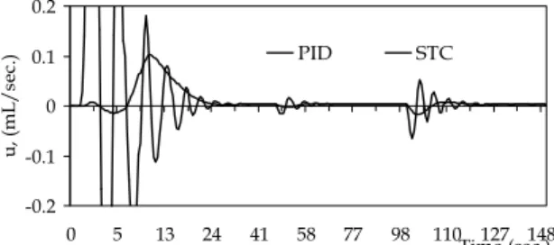
All the PID parameter change is called the self-tuning PID controller due to anticipated nonlinearity and process parameter change. The other test for STCPID is to show the ability to handle the random load HCL (Fa) change as see Fig. 19 and the set point.
Once again, the advantage for STC scheme can see in Fig. 20. At Fig. 20a the random load and set point will automatically updating the process parameter by estimator. The updating and retuning run with recursive to send the proper control signal for pH control systems via open and closed the control valve.
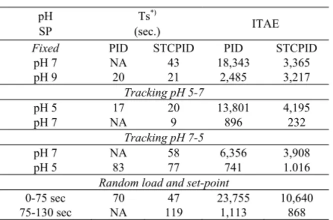
The qualitative performance for all control strategy is calculated by performance index standard. It is shown in Table 1 (settling time Ts and ITAE). The index performance with various set-point change is calculated by average value each reference. The better settling time (Ts) is reached by STC than PID scheme and fastest to achieving pH 7. The NA is abbreviation for Not Available for achieving the pH reference. At pH set point 7 the PID cannot have the Ts and STC reach the 43, 58 second. For the other set point 7, 5 and 9 the STC better than PID with the 43 s, 3s and 1 second in the difference. The ITAE is used to measure the qualitative (minimum energy) for all the time simulation consumption. For pH 7,5 and 9 STC has a good performance comparing with PID it has 15,000, 11,000 in the difference value.
In pH 9 the ITAE PID (2,485) is better than STC (3,217). The all result show that the reaction invariant and STC can be performed a good result due to nonlinearity and pH process parameter change.
TABLE 1. THE PERFORMANCE INDEXES
pH SP
Ts*)
(sec.) ITAE
Fixed PID STCPID PID STCPID
pH 7 NA 43 18,343 3,365
pH 9 20 21 2,485 3,217
Tracking pH 5-7
pH 5 17 20 13,801 4,195
pH 7 NA 9 896 232
Tracking pH 7-5
pH 7 NA 58 6,356 3,908
pH 5 83 77 741 1.016
Random load and set-point
0-75 sec 70 47 23,755 10,640
75-130 sec NA 119 1,113 868
0 2 4 6 8 10 12
0.00 0.01 0.11 0.31 0.62 1.01
Vol. NaOH (mL)
pH
Ka1 Ka2
Ka3
Fig. 6. Titrating H3PO4 with NaOH
Fig. 7. pH curve H3PO4 titrating with various NaOH flowrate
Fig. 8. Reaction invariant variable (xa, xb) for Reaction Fig. 7
0 2 4 6 8 10 12
0 8 19 36 63 87 111 136
(sec.)
pH
PID
set-point STC
PID
(a)
2 4 6 8 10
0 6 15 26 45 68 89 109 128 150
(sec.)
pH
set-point
STC PID
(b)
Fig. 9. pH response (a) set-point pH 7 (b) set-point pH 9
-2 0 2
0 5 11 19 30 43 63
(sec.)
u (
m
L/
se
c.
)
PID STC
Fig. 10. Base (NaOH) flowrate for pH 7
-0.0006 -0.0002 0.0002 0.0006
0 5 11 19 30 43
(sec.) xb (mol)
xa(mol)
Fig. 11. Reaction invariant (xa,xb) for PID Control set-point pH 7
-0.0004 -0.0002 0 0.0002 0.0004 0.0006 0.0008
0 5 11 19 30 43
xb (mol)
xa(mol)
(sec.) Fig. 12. Reaction invariant (xa,xb) for STCPID Control
2 4 6 8 10
0 5 13 24 41 64 80 94 117 138
(sec.)
pH set-point
PID STC
Fig. 13. Set-point tracking pH 9-5
2 3 4 5 6 7 8 9 10 11
0 5 13 24 41 64 78 96 118 138
(sec.)
pH
PID
STC set-point
Fig. 14. Set-point tracking pH 5-7
2.00 4.00 6.00 8.00 10.00
0 5 13 24 41 63 82 102 121 142
(sec.)
pH
PID set-point STC
-0.2 -0.1 0 0.1 0.2
0 5 13 24 41 58 77 98 110 127 148Time (sec.)
u,
(m
L/
se
c.
) PID STC
Fig. 16. The control action u (NaOH Flowrate, Fb, mL/sec.)
-2 -1 0 1 2
0 30 60 90 120 150
(sec.)
θ1 θ3
(a)
-0.045 -0.015 0.015 0.045
0 50 100 150
(sec.) θ2
θ4
(b)
Fig. 17. The parameter estimation due to load change Fig. 14 (a) θ1 & θ3 (b) θ2 &, θ4
0 400 800 1200
0 30 60 90 120 150 (sec.)
Kp
(a)
0 0.2 0.4 0.6 0.8
0 30 60 90 120 150 (sec.) Ti
TD
(b)
Fig. 18. The PID parameter change using STC (a) Kp (b) Ti and TD
V.CONCLUSION
In this paper the reaction invariant with electro neutrality balance is used to modeling the nonlinear mathematical pH model or neutralization process. In this scheme, the Self Tuning Controller (STC) with based PID scheme is done well choose the controller action according to set point and load (disturbance) in pH process.
The advantage was shown to updating automatically PID parameter (Kp, Ti and TD) The simulation results
satisfactory performing to 2%-5% steady state error and well done to track the fixed or set-point change (tracking the set-point). The advantage the STC is not need the large time and ITAE reach the minimum value.
VI.REFERENCES
[1] Fjeld., Asbjørnsen, O. A., Åström, K. J., 1974, Reaction Invariants and Their Importance in The Analysis of Eigenvectors, State Observability and Controllability of The Continuous Stirred Tank Reactor, Chem. Eng. Sci., 29.
0 20 40 50 90 100
170 180 190 200
Fa
H
C
l (
m
L/
se
c.
) (x 10-4)
sec. Fig. 19. Random load (HCl, Fa) change
2 4 6 8 10
0 7 15 28 47 68 83 96 119 138
(sec.)
pH
PID set-point STC
(a)
-0.5 -0.3 -0.1 0.1 0.3 0.5
0 15 47 83 119
PID STC
(sec.)
u (m
L/
se
c.
)
(b)
Fig. 20. STC pH response for random load and set-point change (a) pH output (b) control signal u (Fb, mL/sec.)
[2] Waller, K. V., Mäkilä, P. M., 1981, Chemical Reaction Invariants and Variants and Their Use in Reaction Modeling, Simulation, and control, Ind. Eng. Chem. Process Des. Dev., 20, 1- 11. [3] Gufftafson, T.K, and Waller, K.V., 1983, Dynamic Modeling and
Reaction Invariant Control pH, Chemical Engineering Science, Vol.38, pp.389-398.
[4] Cordova, H., 2003, Prototype Kontroler PID Self-Tuning Menggunakan Algoritma Auto-Switch Berbasis Margin Fasa dan Penguatan pada Proses Penetralan pH Larutan Campuran NaOH dan HAC, [Laporan Akhir Penelitian DIKS ITS 2003] Lembaga Penelitian dan Pengabdian Pada Masyarakat –ITS.
[5] Cordova, H., 2005, PID Control Systems Design to pH Neutralization by Neural Network Inverse Model Optimization at PT Petrokimia-Gresik, Prosiding Seminar FTI-ITS: Deindsutrialisasi Nasional: Ancaman Terhadap Pengembangan Daya Saing Global, hal. 20-22, Surabaya, Indonesia.
[6] Cordova, H., 2005, The Application of Early Warning System for Monitoring and Control pH Water Based On Auto-Switch Algorithm, Prociding International Seminar and Disaster for Early Warning Systems PSB-ITS, 4-5 March, pp.10-13, Surabaya, Indonesia.
[7] Cordova, H., 2004, PID Self-Tuning Based on Auto-Switch Algorithm to Control pH Neutralization Process, Jurnal Industri, FTI-ITS, Vol. 3, hal.3-6.
[8] Ishak., A,A., Hussain., M,A., 2001, Modeling and Control Studies of Waste Water Treatment Process., Proceeding to Brunei International Conference on Engineering & Technology, Bandar Seri Begawan, 9- 11 Oct, pp. 221-231.
[9] Besharati, R, A., Lo, W, W., Tsang, K, M., 2001, Self-tuning PID Controller Using Newton-Raphson Method, IEEE Transaction On Industrial Electronic, Vol. 44, no.5, pp. 432-440.
[10] Manzi, J.T.; Odloak, D., 1998, Control and Stability Analysis GMC Algorithm Applied to pH System, Braz. J. Chem. Eng. v. 15 n. 3 São Paulo Sept, pp.15-20, http:// www.scielo.br/scielo.php?Ing=es [2 September].
[11] McAvoy, T., Hsu, E., Lowenthal, S., 1972, Dynamics of pH in Controlled Stirred Tank Reactor, Ind. & Eng. Chem., Process Descr. & Develop. 11(1), 67-70, 1972.
[13] Cordova, H., 2006, Prototipe Kontroller Intelligent Self-Tuning PID pada Proses Penetralan pH dengan Metode Penalaan Newton-Rhapson, [Laporan Akhir Penelitian DIKS ITS 2006] Lembaga Penelitian dan Pengabdian Pada Masyarakat –ITS. [14] Cordova, H., Wijaya., AF., 2007, Self-Tuning PID Neural
Network Controller to Nonlinear pH Neutralization on Waste Water Treatment, Jurnal IPTEK, ITS, vol. 18, n. 3, hal. 5-10. [15] Astrom, K.J., Wittenmark, B., 1995, “Adaptive Control”, Addison
Wesley Publishing Company, USA., Page 150-250.
[16] Bobál, V, Böhm, J, Fessl, J, Macháéca’k, J., 2005, Digital Self Tuning Controllers., Springer-Verlag., London., UK., Page. 130-225.
[17] Ylén, J-P., Measuring, 2001, Modeling and Controlling The pH Value and The Dynamic Chemical State., [Dissertation for the degree of Doctor], Department of Automation and Systems Technology., Helsinki University of Technology.
[18] Boling., J,M., Seborg., D,E., Hespanha, J,P., 2006, Multi-Model Adaptive Control of a Simulated pH Neutralization Process,
Elsevier Science., Vol. 3. no. 2. pp. 240-250.
[19] Henson, M.A., Serborg, D.E., 1998, “Adaptive Nonlinear Control of a pH Neutralization Process,” IEEE Transaction on Control Systems Technology, vol. 2, no. 3 August.
Appendix
The closed loop pH control system in the Continuous Stirred Tank Reactor schematic,
The STCPID received the pH process value from pH sensor, and calculated the proper signal action u(t) L/sec. for Base (Fb,Cb) NaOH