Int. J. of Mathematical Sciences and Applications, Vol. 2, No. 2, May 2012
Copyright
Mind Reader Publicationswww.journalshub.com
STOCHASTIC PERISHABLE INVENTORY CONTROL SYSTEMS IN
SUPPLY CHAIN WITH PARTIAL BACKORDERS
R.Bakthavachalam 1* S.Navaneethakrishnan 2 C. Elango3
1
Department of Mathematics, Raja College of Engineering & Technology, Madurai,TN.
2
Department of Mathematics, V.O.C College, Thoothukudi, TN.
3
Department of Mathematical Sciences, C.P.A College Bodinayakanoor, TN.
Abstract
This article analyzes a supply chain management system (SCM), with two echelons. We consider a perishable inventory with Poisson demand, exponential life time and positive lead time at distribution center (DC) and retailer. Partial backlogging at retailer node is assumed with limited quantity. (s, S) policy at retailer and (M-1, M) policy at DC are assumed to get a tractable analytic solution. Transient and steady state solutions are discussed. Numerical examples are provided to illustrate the proposed SCM model.
Keywords: Supply chain management, Multi-echelon Inventory control, perishable inventory control, Optimization.
AMS Classification Number: 90B05, 60J27, 91B70
1. Introduction
The study of supply chain management started in the late 1980s and has gained a growing level of interest from both companies and researchers over the past three decades.
There are many definitions of supply chain management. Hau Lee, the head of the Stanford Global Supply Chain Management Forum (1999), gives a simple and straight forward definition at the forum website as follows: ‘Supply chain management deals with the management of materials, information and financial flows in a network consisting of suppliers, manufacturers, distributors, and customers’. From this definition, we can see that SCM is not only an important issue to manufacturing companies, but is also relevant to service and financial firms. A supply chain may be defined as an integrated process wherein a number of various business entities (suppliers, distributors and retailers) work together in an effort to (1) acquire raw materials (2) process them and then produce valuable products and (3)transport these final product to retailers. The process and delivery of goods through this network needs efficient maintenance of inventory, communication and transportation system. The supply chain is traditionally characterized by a forward flow of materials and products and backward flow of information, money, etc.
One of the most important aspects of supply chain management is inventory control. Inventory control models are almost invariably stochastic optimization problems with an objective function being either expected costs or expected profits or risks. In practice, a retailer may want an optimal decision which achieves a minimal expected cost or a maximal expected profit with low risk of deviating from the objective
Perishable goods are those goods, which have a fixed or specified lifetime after which they are considered unusable, that is they cannot be utilized to meet the demand. The planning and control of perishable inventory systems is important because in real life products like milk, blood, drug, food, vegetables and some chemicals do have fixed life times after which they will perish. The presence of these kind products after their
lifetime will not only occupy space of the store, but also affect the lifetime (damage) of the neighboring items. The decayed (exponential decay) items may be removed from the stock at certain time points.
A complete review was provided by Benita M. Beamon (1998) [4]. However, there has been increasing attention placed on performance, design and analysis of the supply chain as a whole. HP's (Hawlett Packard) Strategic Planning and Modeling (SPaM) group initiated this kind of research in 1977. From practical stand point, the supply chain concept arose from a number of changes in the manufacturing environment, including the rising costs of manufacturing, the shrinking resources of manufacturing bases, shortened product life cycles, the leveling of planning field within manufacturing, inventory driven costs (IDC) involved in distribution (2005) and the globalization of market economics. Within manufacturing research, the supply chain concept grow largely out of two-stage multi-echelon inventory models, and it is important to note that considerable research in this area is based on the classic work of Clark and Scarf (1960) [6]. A complete review on this development was recorded by Federgruen (1993) [9]. Recent developments in two-echelon models may be found in Axaster, S (1993) [3], Nahimas, S (1982) [13] and Antony Svoronos & Paul Zipkin (1991) [1]. Continuous review Perishable inventory with instantaneous replenishment at single location was considered by Kalpakam, S and Arivarignan, G (1988) [10]. Continuous review Perishable inventory at service facility has been studied by Elango.C (2000) [8] and Arivarignan.G, Elango.C and Arumugam (2002) [2].
A continuous review (s, S) policy with Poisson demands and positive lead times in two-level Inventory Control in Supply Chain was considered by Krishnan. K (2007) [11]. In our previous papers we are discussed three level stochastic inventory control models with lost sale model for both perishable and non-perishable products [14, 15]. Now we extended the model to introduce partial backorder that is the demands occurring during the stock out periods at retailer node are backlogged upto ‘b’ units. This paper deals with a simple supply chain that is modeled as system with a single warehouse, a distribution center and single retailer, handling a single product. In order to avoid the complexity, at the same time without loss of generality, we assumed the Poisson demand pattern at retailer node. This restricts our study to design and analyze as the tandem network of inventory, which is the building block for the whole supply chain system.
The rest of the paper is organized as follows; the model formulation is described in section 2. In section 3, both transient and steady state analysis are done. Section 4, deals the derivation of operating characteristics of the system and section 5, deals with the cost analysis for the operation. Numerical examples and sensitivity analysis are provided in section 6 and the last section 7 concludes the paper.
2. The Model Description
For over 50 years researchers have been addressing a variety of problems in multi-echelon inventory systems. The current research is unique and distinct from previous research because it combines all of the following features (assumptions):
We consider a three level supply chain system consisting of a warehousing facility, single distribution centre and one retailer dealing with a single perishable product.
Figure 1-Tandem Network Inventory Control System in Supply Chain
A perishable product is supplied from warehouse to distribution center which adopts one-for-one replenishment policy (M-1, M). The product is supplied from distribution center to the retailer who adopts (s, S) policy. The demand at retailer node follows a Poisson process with rate λ >0. Supply to the retailer in packets of Q (=S-s) items is administrated with exponential lead time having parameter µ>0.The replenishment of items in
µ1 S M WH DC R
Demands occurring during the stock out periods are backlogged upto a specified quantity ‘b’ at retailer node. [Where b is the backorder level such that Q > b + s , that is Q-s > b>0 ]. A demand at distribution center (Q items) is satisfied by local purchase during the shortage at distribution center. The maximum inventory level at retailers node S is fixed and the maximum inventory level at distribution centre is M a variable quantity (M = nQ; Q = S-s, n∈N).
According to the above assumptions the on hand inventory levels at both nodes are random variables, and yields a two dimensional stochastic process.
We fix the following notations for the forthcoming analysis part of our paper. [R]ij : the element /sub matrix at (i,j)th position of R
0 : zero matrix of appropriate dimension I : an identity matrix of appropriate dimension . e : a column vector of 1’s of appropriate dimension.
3. Analysis
Let I0(t) denote the on hand inventory level at retailer node and I1(t) denote the on hand inventory level
at distribution centre node at time t+. From the assumptions on the input and output processes , I (t) = {(I0 (t), I1
(t)) : t ≥ 0 } is a Markov process with state space E = {(j, q) / j = S, S-1 …3, 2, 1, 0, -1,-2,-3 … -b. and q = 0,Q, 2Q…nQ}. Where b is backorder level such that Q > b + s. that is Q - s > b ≥ 0.(we use negative sign for backlogging quantity)
The infinitesimal generator of this process
A
=
(
a
(
j
,
q
:
k
,
r
))
(
j
,
q
)(
k
,
r
)
∈
E
can be obtained using the following arguments.• The arrival of a demand of an item or perish makes a transition in the Markov Process from (j, q) to (j-1, q) with intensity of transition λ (> 0) or (γ >0).
• Replenishment of inventory at retailer node makes a transition from (j, nQ) to (j +Q, (n-1)Q) with rate of transition µ > 0.
• Replenishment of inventory at distribution centre node makes a transition from (j,M-Q) to (j,M) with rate of transition µ1 (> 0).
The infinitesimal generator R is given by
−
−
=
E
C
0
...
0
0
0
B
D
C
...
0
0
0
...
...
...
...
...
...
0
0
0
...
D
C
0
0
0
0
...
B
D
C
0
0
0
...
0
B
A
0
Q
...
Q
)
2
n
(
Q
)
1
n
(
nQ
R
The entries of the matrix R can be written as
=
=
=
=
+
=
=
=
=
=
=
=
otherwise
0
q
r
;
0,
q
if
E
Q
r
;
Q
2)Q...2Q,
-(n
1)Q,
-n
(
q
if
D
Q
q
r
;
Q,0
2)Q...2Q,
-(n
1)Q,
-(n
q
if
C
Q
-q
r
;
Q
2)Q...2Q,
-(n
1)Q,
-(n
,
nQ
q
if
B
q
r
;
nQ,
q
if
A
[R]
q
x
r
Then the sub matrices A, B, C, D and E are given by
=
=
µ
λ
+
µ
=
=
+
=
=
µ
+
γ
+
λ
+
=
=
γ
+
λ
=
=
λ
=
=
γ
+
λ
otherwise.
0
0
j
j,
q
if
-1).
-b
0,-1,-2,-(
j
j,
q
if
)
(
-2,1.
...
2,
-s
1,
-s
s,
j
j,
q
if
)
i
(
-1).
(s
...
2,
-S
1,
-S
S,
j
j,
q
if
)
i
(
-.
1)
-(b
-.
0,-1,-2,..
j
1,
-j
q
if
.
2,1
...
2,
-S
1,
-S
S,
j
1,
-j
q
if
i
=
[A]
j
x
q
µ
=
+
=
−
−
otherwise
0
.
b
--1,-2,...
,
0
,
1
,
2
,...
2
s
,
1
s
,
s
j
Q
j
q
if
=
[B]
j
x
q
µ
=
=
−
−
−
−
otherwise
0
.
b
--1,-2,...
,
0
,
1
,
2
,...
2
s
,
1
s
,
s
,...
2
S
,
1
S
,
S
j
j
q
if
=
[C]
j
x
q
1
=
=
µ
+
µ
λ
+
µ
+
µ
=
=
+
=
=
µ
+
µ
+
γ
+
λ
+
=
=
µ
+
γ
+
λ
=
=
λ
=
=
γ
+
λ
otherwise.
0
0
j
j,
q
if
)
(
-1).
-b
0,-1,-2,-(
j
j,
q
if
)
(
-2,1.
...
2,
-s
1,
-s
s,
j
j,
q
if
)
i
(
-1).
(s
...
2,
-S
1,
-S
S,
j
j,
q
if
)
i
(
-.
1)
-(b
-.
0,-1,-2,..
j
1,
-j
q
if
.
2,1
...
2,
-S
1,
-S
S,
j
1,
-j
q
if
i
=
[D]
1
1
1
1
q
x
j
=
=
µ
λ
+
µ
=
=
+
=
=
µ
+
γ
+
λ
=
=
λ
=
=
γ
+
λ
otherwise.
0
0
j
j,
q
if
-1).
-b
0,-1,-2,-(
j
j,
q
if
)
(
-2,1.
...
2,
-S
1,
-S
S,
j
j,
q
if
)
i
(
-.
1)
-(b
-.
0,-1,-2,..
j
1,
-j
q
if
.
2,1
...
2,
-S
1,
-S
S,
j
1,
-j
q
if
i
=
[E]
1
1
1
q
x
j
3. 1 Transient AnalysisLet I0 (t) and I1 (t) denote the on hand inventory levels at retailer node and distribution node respectively
at time t+. From the assumptions on the input and output processes, clearly the vector process {I(t) : t ≥ 0} where I(t) = (I0(t), I1(t)) for t ≥ 0 is a continuous time Markov Chain with state space E = {(j, q) / j = 0, 1, 2..., S ; q =
0,Q, 2Q, ...,nQ}. Define the transition probability function: Pj,q(k, r : t) = Pr {(I0(t), I1(t)) = (k, r) | (I0(0), I1(0)) = (j,
q)}.The corresponding transient matrix function is given by P(t) = (Pj,q(k, r : t))(j,q)(k,r)∈ E which satisfies the
Kolmogorov forward equation P’(t) = P(t)A, where A is an infinitesimal generator. Above equation, together with initial condition P(0) = I, yields a solution of the form P(t) = P(0)eAt = eAt where the matrix expansion in power series form is ∞∑ = + = 1 n n n At n! t A I e .
Case (i): Suppose that the eigen values of A are all distinct. Then from the spectral theorem of matrices, we have A = HDH−1, where H is the non-singular ( formed with the right eigen vectors of A) and D is the diagonal matrix having its diagonal elements, the eigen values of A. Now 0 is an eigen value of A and if di ≠ 0, i = 1, 2, ...,m, are
the distinct eigen values then we have An = HDnH−1. Using An in P(t) we have the explicit solution of P(t) as P(t) = HeDtH−1 with
=
−
t
m
d
t
1
m
d
t
1
d
Dt
e
..
..
..
0
0
e
..
0
0
...
..
..
...
...
...
..
..
e
0
0
..
..
0
1
e
and
=
−
m
1
m
1
d
..
..
..
0
0
d
..
0
0
...
..
..
...
...
...
..
..
d
0
0
..
..
0
0
D
Case (ii): Suppose the eigen values of A are all not distinct, we can find a canonical representation as A = SZS−1. From this the transition matrix P(t) can be obtained in a modified form. (Medhi, J [12]).
3.2 Steady State Analysis:
The structure of the infinitesimal matrix R reveals that the state space E of the Markov chain {I(t) : t ≥ 0}, is finite and irreducible. Let the limiting distribution of the inventory level process be defined
by
{
}
E ) q , j ( 1 0 t q jlim
Pr
(
I
(
t
),
I
(
t
))
(
j
,
q
)
P
∈ ∞ →=
=
where Pjq is the steady state probability that the system be in state (j,q), (Cinlar [5].Let
ν
=
(
ν
nQ
,
ν
(
n
−
1
)
Q
,
ν
(
n
−
2
)
Q
...
ν
Q
,
ν
0
)
denote the steady state probability distribution where
ν
ν
ν
=
ν
−
q
0
q
1
S
q
S
q
,
....
for the system under consideration. For each (j, q), νqj can be obtained by solving
the matrix equation νR = 0, that is the steady state balance equations are
νiQ A + ν(i-1)QC = 0 ; i= n νiQ B + ν(i-1)QD + ν(i-2)QC = 0 ; i= n,n-1,.n-2,…2 νiQ B + ν(i-1)QE = 0 ; i= 1, together with normalizing condition
∑
ν
=
q
,
j
q
j
1.
4. OPERATING CHARACTERISTICS 4.1 Reorder Rate:Consider the event βi of reorders at node i (i =0,1). Observe that β0 - events occur whenever the inventory level at retailer node reaches s, whereas the β1-event occurs whenever the inventory level at distribution centre reaches (M-Q).
The mean reorder rate at retailer node is β0 and the mean reorder rate at the distribution centre is β1 Thus
∑
=
+
λ
=
β
nQ
Q
q
q
1
s
0
P
and∑
−
=
=
µ
=
β
s,
(
n
1
)
Q
0
q
,
0
j
q
j
1
P
4.2 Mean Inventory Level:
Let
Ii
denote the mean inventory level in the steady state at node i (i=0,1). Thus,∑
=
∑
=
=
nQ
Q
q
S
0
j
q
j
0
.j
p
I
and∑
=
=
∑
=
S
0
j
nQ
Q
q
q
j
1
q
.
p
I
4.3 Shortage rate:Shortage occurs at retailer nodes and only upto ‘b’ units are backlogged, the remaining demands are assume to be lost sale. Therefore the shortage rate at retailer node (α0)is given by
∑
=
λ
=
α
nQ
Q
q
q
b
0
P
and thedemand at distribution center ) is satisfied by local purchase during the stock out period, hence the shortage rate at distribution centre (α1) is given by
∑
=
µ
=
α
s
0
j
0
j
1
P
. 5 COST ANALYSISIn this section we impose a specified cost structure for the proposed model. Considering the minimization of the long run total expected cost per unit time. There are fixed ordering costs k1 associated with each order initiated from warehouse to distribution centre and k0 that of initiated from distribution centre to retailer regardless of the order size.
The holding cost h1 per unit of item per unit time at distribution centre and the holding cost h0per unit of item per unit time at retailer node are considered. The demands occur during stock out period are assumed as lost.
g0 and g1 are theshortage costper unit shortage at retailer node and distribution centre respectively. The long run expected cost rate C(s,Q) is given by
1 1 0 0 1 1 0 0 1 1 0 0I h I k k g g h ) Q , s ( C = + + β + β +α +α ,
where hi is the holding cost at node i, ki is the setup cost for node i and gi is the shortage cost at node i
(i=0,1) for unit shortage. Although we have not proved analytically the convexity of the cost function C(s,Q), our experience with considerable number of numerical examples indicates that C(s,Q) for fixed Q to be convex in s. In some cases it turned out to be an increasing function of s. Hence we adopted the numerical search procedure to determine the optimal values s*, consequently we obtain optimal n* =
*
Q
M
.For large number of parameters, our calculation of C(s, Q) revealed a convex structure for the same. Hence we adopted a numerical search procedure to obtain the optimal value s* for each S.
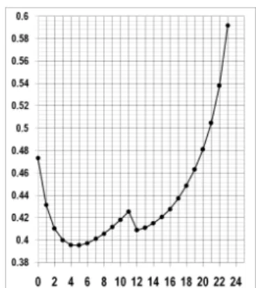
6. Numerical Exampleand Sensitivity Analysis
In this section we discuss the problem of minimizing the long run total expected cost per unit time under the following cost structure. The results we obtained in the different cases may be illustrated through the following numerical example.
For the input S= 24, b= 2, M= 5, µ1=0.1, h0=0.005, h1=0.003, λ0=0.9, µ = 0.2, k0=1.75, k1=0.5, g0 =0.3, g1
=0.5, γ =0.4.
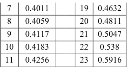
Table 1 - The total expected cost rate as a function of C(s,Q) s Cost s Cost 0 0.4733 12 0.4089 1 0.4316 13 0.4111 2 0.4104 14 0.4153 3 0.4001 15 0.4207 4 0.3958 16 0.4276 5* 0.3954* 17 0.4372
7 0.4011 19 0.4632 8 0.4059 20 0.4811 9 0.4117 21 0.5047 10 0.4183 22 0.538 11 0.4256 23 0.5916
For each of the inventory capacity S, the optimal reorder level‘s’ and optimal cost C(s,Q) are indicated by the symbol ’*’.
Sensitivity Analysis – 1. For the same input with reorder at s = 5.
Table 2- The total expected cost deviation based on various holding cost (h0 and h1) h0 h1 1 2 3 4 5 1 5.3617 5.6014 5.8411 6.0808 6.3205 2 10.1038 10.3435 10.5832 10.8229 11.0626 3 14.8459 15.0856 15.3253 15.5650 15.8047 4 19.5580 19.8277 20.0674 20.3071 20.5468 5 24.3301 24.5698 24.8094 25.0491 25.2888
It is observed that if the holding cost (h0 and h1) of the item is increased then the total expected cost C(s, Q) is also
increased. Hence the holding cost is key parameter of this system. Sensitivity Analysis – 2. For the same input with reorder at s = 5.
Table 3- The total expected cost deviation based on various demand rate λλλλ0 λλλλ0 C(s,Q) 1 5.3617 2 10.1038 3 14.8459 4 19.5580 5 24.3301
It is observed that if the demand rate is increased then the total expected cost C(s,Q) is also increased.
7. Concluding remarks
In this paper we analyzed a continuous review perishable inventory control system strategy to Multi-echelon system. The structure of the chain allows vertical movement of goods from warehouse to Distribution center to then retailers. The model is dealing the supply from distribution center is in the terms of pockets. We are also proceeding in this multi-echelon stochastic inventory control system with non-perishable products and also dealing with backlogging. This model deals with only tandem network (basic structure of supply chain), this structure can be extended to tree structure and to be more general.
REFERENCES
[1] Antony Svoronos and Paul Zipkin, Evaluation of One-for-One Replenishment Policies for Multiechelon Inventory Systems, Management Science, 37(1): 68-83, 1991.
[2] Arivarignan. G, Elango. C and Arumugam. N, A continuous review perishable inventory control system at service facilities, Advances in Stochastic Modelling, Notable Publications, Inc., 29 – 40, 2002.
[3] Axaster, S. Exact and approximate evaluation of batch ordering policies for two level inventory systems. Operation Research 41. 777-785, 1993.
[4] Benita M. Beamon, Supply Chain Design and Analysis: Models and Methods. International Journal of Production Economics.Vol.55, No.3, pp.281-294, 1998.
[5] Cinlar. E, Introduction to Stochastic Processes. Prentice Hall, Englewood Cliffs, NJ, 1975.
[6] Clark A J and Scarf H, Optimal Policies for a Multi- Echelon Inventory Problem. Management Science, 6(4), 475-490, 1960.
[7] Diwakar Gupta and Selvaraju.N Performance evaluation and stock allocation in capacitated serial supply system, Manufacturing & service-operations management vol.8 No.2 INFORMS. PP 169-191, 2006. [8] Elango, C., A continuous review perishable inventory system at service facilities, unpublished Ph. D.,
Thesis, Madurai Kamaraj University, Madurai, 2000.
[9] Federgruen. A, Centralized planning models for multi echelon inventory system under uncertainty, S.C.Graves et al.eds. Handbooks in ORMS vol 4, North-Holland, Amsterdam, The Netherlands, 133-173, 1993.
[10] Kalpakam, S and Arivarignan, G. A Continuous review Perishable Inventory Model, Statistics 19, 3, 389-398, 1988.
[11] Krishnan.K, Stochastic Modeling in Supply Chain Management System, unpublished Ph.D., Thesis, Madurai Kamaraj University, Madurai, 2007.
[12] Medhi, J.: Stochastic processes. new age international publishers. India, 2009.
[13] Nahimas S, Perishable inventory theory a review. Operations Research, 30, 680-708, 1982.
[14] Bakthavachalam, R. and Elango, C. Multi-Echelon Stochastic Inventory Control Systems in Supply Chain, Computational and Mathematical Modelling, Narosa Publishing House, New Delhi. pp191-199, 2011.
[15] Bakthavachalam, R. and Elango, C. Perishable Inventory Control System with Partial Backlogging in Supply Chain, The PMU Journal of Humanities and Science, vol.2, No.2. pp 31-41, 2011.