UDT: UDP-based Data Transfer
for High-Speed Wide Area Networks
Yunhong Gu and Robert L. Grossman
National Center for Data Mining, University of Illinois at Chicago
851 S Morgan St, M/C 249, Chicago, IL 60607, USA
[email protected], [email protected]
Abstract
In this paper, we summarize our work on the UDT high performance data transport protocol in the past four years. UDT was designed to effectively utilize the rapidly emerging high-speed wide area optical networks. It is built on the top of UDP with reliability control and congestion control, which makes it quite easy to get installed. The congestion control algorithm is the major internal functionality to enable UDT to effectively utilize the high bandwidth. Meanwhile, we also implemented a set of APIs to support easy application implementation, including both reliable data streaming and partial reliable messaging. The original UDT library has also been extended to Composable UDT, which can support various congestion control algorithms. We will describe in detail the design and implementation of UDT, the UDT congestion control algorithm, Composable UDT, and the performance evaluation.
Keywords: Transport Protocol, Congestion Control, High Speed Networks, Design and Implementation
1.
INTRODUCTION
The rapid increase of network bandwidth and the emergence of new distributed applications are the two reciprocal motivations of networking research and development. On the one hand, network bandwidth today has been expanded to 10Gb/s with 100Gb/s emerging, which enables many data intensive applications that were impossible in the past. On the other hand, new applications, such as scientific data distribution, expedite the deployment of high-speed wide-area networks.
Today, national or international high-speed networks have connected most developed regions in the world with fibers [13, 17]. Data can be moved at up to 10 Gb/s among these networks and often at a higher speed inside the networks themselves. For example, in the United States, there are national multi-10Gb/s networks, such as National Lambda Rail, Internet2/Abilene, Teragrid, ESNet, etc. They can connect to many international networks such as CA*Net 4 of Canada, SurfNet of the Netherlands, and JGN2 of Japan.
Meanwhile, we are living in a world of exponentially increasing
data. The old way of storing data in disk or tape storage and delivering them by transport vehicles is no longer efficient. In many situations, this old fashioned method of shipping disks with data on them makes it impossible to meet the applications' requirement (e.g., online data analysis and processing).
Researchers in high-energy physics, astronomy, earth science, and other high performance computing areas have started to use these high-speed wide area optical networks to transfer their terabytes of data. We expect that home Internet users will also be able to make use of the high-speed networks in the near future for applications with high-resolution streaming video, for example. In fact, an experiment between two ISPs in USA and Korea has demonstrated an effective 80Mb/s data transfer speed.
Unfortunately, the high-speed networks have not been smoothly used by those applications. The Transmission Control Protocol (TCP), the de facto transport protocol of the Internet, substantially underutilizes network bandwidth over high-speed connections with long delays [13, 22, 39, 70]. For example, a single TCP flow with default parameter settings on Linux 2.4 can only reach about 5 Mb/s over a 1Gb/s link between Chicago and Amsterdam; with careful parameter tuning the throughput still only reaches about 70Mb/s. A new transport protocol as a timely solution is required to address this challenge. The new protocol is expected to be easily deployed and easily integrated with the applications, in addition to utilizing the bandwidth efficiently and fairly.
Network researchers have proposed quite a few solutions to this problem, most of which are new TCP congestion control algorithms [8, 23, 25, 37, 40, 53, 55, 67] and application-level This paper is partly based upon five conference papers published on the
proceedings of PFLDNet workshop 2003 and 2004, IEEE GridNets workshop 2004, and IEEE/ACM SC conference 2004 and 2005. See reference [26, 27, 28. 29, 30].
libraries using UDP [18, 26, 61, 65, 66, 71]. Parallel TCP [1, 56] and XCP [39] are two special cases: the former tries to start multiple concurrent TCP flows to obtain more bandwidth, whereas the latter is a radical change by introducing a new transport layer protocol involving changes in routers.
In UDT we have a unique approach to address the problem of transfer large volumetric datasets over high bandwidth-delay product (BDP) networks. While UDT is a UDP-based approach, to our best knowledge, it is the only UDP-based protocol that employs a congestion control algorithm targeting shared networks. Furthermore, UDT is not only a new control algorithm, but also a new application level protocol with support for user configurable control algorithms and more powerful APIs.
This paper summarizes our work of UDT in the past four years. Section 2 gives an overview of the UDT protocol and describes its design and implementation. Section 3 explains its congestion control algorithm. Section 4 introduces Composable UDT that supports configurability of congestion control algorithms. Section 5 gives an experimental evaluation of the UDT performance. Section 6 concludes the paper.
2.
THE UDT PROTOCOL
2.1
Overview
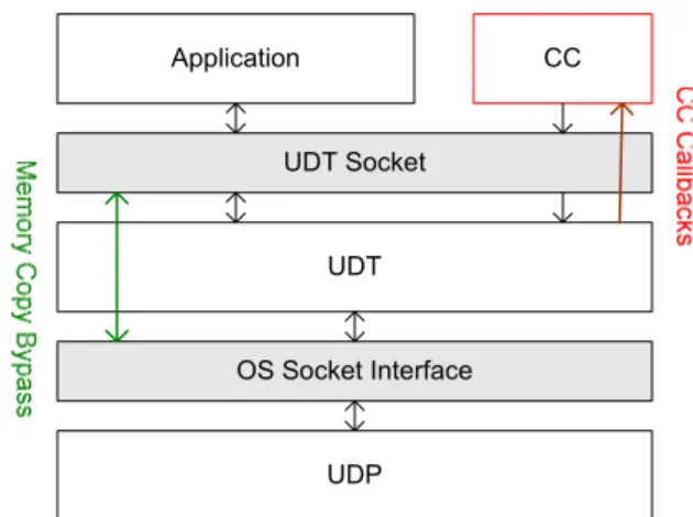
UDT adapts itself into the layered network protocol architecture (Figure 1). UDT uses UDP through the socket interface provided by operating systems. Meanwhile, it provides a UDT socket interface to applications. Applications can call the UDT socket API in the same way they call the system socket API. An application can also provide a congestion control class instance (CC in Figure 1) for UDT to process the control events, thus a customized congestion control scheme will be sued, otherwise the default congestion control algorithm of UDT will be used.
UDP OS Socket Interface
UDT UDT Socket
Application CC
Figure 1: UDT in the Layer Architecture. UDT is in the application layer above UDP. Application exchanges its data through UDT socket, which then uses UDP socket to send or receive the data. Memory copy is bypassed between UDT socket and UDP socket, in order to reduce processing time. Application can also provides a customized control scheme (CC).
UDT addresses two orthogonal research problems: 1) the design and implementation of a transport protocol with respect to functionality and efficiency; and, 2) an Internet congestion
control algorithm with respect to efficiency, fairness, and stability.
In this section, we will describe the design and implementation of the UDT protocol (Problem 1). The congestion control algorithm and the Composable UDT (Problem 2) will be introduced in Section 3 and Section 4, respectively.
2.2
Protocol Design
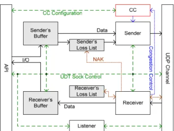
UDT is a connection-oriented duplex protocol, while it supports both reliable data streaming and partial reliable messaging. Figure 2 describes the relationship between the UDT sender and the receiver. In Figure 2, the UDT entity A sends application data to the UDT entity B. The data is sent from A’s sender to B’s receiver, whereas the control flow is exchanged between the two receivers.
Figure 2: Relationship between UDT sender and receiver. All UDT entities have the same architectures, each having both a sender and a receiver. This figure demonstrates the situation when a UDT entity A sends data to another UDT entity B. Data is transferred from A’s sender to B’s receiver, whereas control information is exchanged between the two receivers.
The receiver is also responsible for triggering and processing all control events, including congestion control and reliability control, and their related mechanisms as well.
UDT uses rate-based congestion control (rate control) and window-based flow control to regulate the outgoing data traffic. Rate control updates the packet-sending period every constant interval, whereas flow control updates the flow window size each time an acknowledgment packet is received.
2.2.1
Packet Structures
There are two kinds of packets in UDT: the data packets and the control packets. They are distinguished by the 1st bit (flag bit) of the packet header.
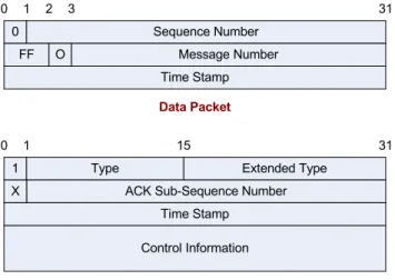
A UDT data packet contains a packet-based sequence number, a message sequence number, and a relative timestamp (which starts counting once the connection is set up) in the resolution of microseconds (Figure 3), in addition to the UDP header information.
Note that UDT’s packet-based sequencing with the packet size information provided by UDP is equivalent to TCP’s byte-based sequencing and can also support data streaming. Meanwhile, the message sequence number is only used for messaging services. The message number field indicates which packets consist of a particular application message. A message may contain one or more packets. The "FF" filed indicates the message boundary: first packet – 10, last packet – 01, and solo packet – 11. The "O" filed indicates if this message should be delivered in order.
In-order delivery means that the message cannot be delivered until all messages prior to it are whether delivered or dropped.
0 Sequence Number
FF O Message Number
Time Stamp
0 1 2 3 31
Data Packet
1 Type Extended Type
ACK Sub-Sequence Number X
Time Stamp Control Information
Control Packet
0 1 15 31
Figure 3: UDT packet header structures. The first bit of the packet header is a flag to indicate if this is a data packet (0) or a control packet (1). Data packets contain a 31-bit sequence number, a 29-bit message number, and a 32-bit timestamp. In the control packet header, bit 1- 15 is the packet type information and bit 16 –31 can be used for user-defined types. The detailed control information depends on the packet type.
There are 7 types of control packets in UDT and the type information is put in bit field 1 - 15 of the packet header. The contents of the following fields depend on the packet type. The first three 32-bit fields must exist in the packet header, whereas there may be an empty control information field, depending on the packet type.
Particularly, UDT uses sub-sequencing for ACK packet. Each ACK packet is assigned a unique increasing 31-bit sequence number, which is independent of the data packet sequence number.
The 7 types of control packets are: handshake (connection setup information), ACK (acknowledgment), ACK2 (acknowledgment of acknowledgment), NAK (negative acknowledgment, or loss report), keep-alive, shutdown, and message drop request.
The extended type field is reserved for users to define their own control packets in the Composable UDT framework (Section 4).
2.2.2
Connection Setup and Teardown
UDT supports two kinds of connection setup, traditional client/server mode and rendezvous mode.
In the client/server mode, one UDT entity starts first as the server, and its peer side (the client) that wants to connect to it will send a handshake packet first. The client should keep on sending the handshake packet every constant interval (the implementation should decide this interval according to the balance between response time and system overhead) until it receives a response handshake from the server or a time-out timer expires.
The handshake packet has the following information: 1) UDT version, 2) socket type (SOCK_STREAM or SOCK_DGRAM),
3) initial random sequence number, 4) maximum packet size, and 5) maximum flow window size.
The server, when receiving a handshake packet, checks its version and socket type. If the request has the same version and type, it compares the packet size with its own value and sets its own value as the smaller one. The result value is also sent back to the client by a response handshake packet, together with the server's initial sequence number and maximum flow window size. The server is ready for sending/receiving data right after this step. However, it must send back a response packet as long as it receives any further handshakes from the same client, in case the client does not receive the previous response.
The client can start sending/receiving data once it gets a response handshake packet from the server. Further response handshake messages, if any are received, should be omitted.
Traditional client/server setup process requires explicit server side and client side. However, this mechanism does not work if both of the machines are behind firewalls, when the connection setup request from the client side will be dropped.
In order to support convenient connection setup in this situation, UDT provides the rendezvous connection setup mode, in which there is no server or client, and two users can connect to each other directly.
Inside the UDT implementation of the rendezvous connection setup, each UDT socket sends connection request to its peer side, and whoever receives the request will then send back response and set up the connection.
If one of the connected UDT entities is being closed, it will send a shutdown message to the peer side. The peer side, after receiving this message, will also be closed. This shutdown message, delivered using UDP, is only sent once and not guaranteed to be received. If the message is not received, the peer side will be closed by a timeout mechanism (through the keep-alive packets). Keep-alive packets are generated periodically if there is no other data or control packets sent to the peer side. A UDT entity can detect a broken connection if it does not receive any packets in a certain time.
2.2.3
Reliability Control / Acknowledging
Acknowledgment is used in UDT for congestion control and data reliability. In high-speed networks, generating and processing acknowledgments for every received packet may take a substantial amount of time. Meanwhile, acknowledgment itself also consumes some bandwidth. (This problem is more serious if the gateway queues use packets rather than bytes as the minimum processing unit, which is very common today.)
UDT uses timer-based selective acknowledgment, which generates an acknowledgment at a fixed interval, if there are new continuously received data packets. This means that the faster the transfer speed, the smaller the ratio of bandwidth consumed by control traffic. Meanwhile, at very low bandwidth, UDT acts like protocols that acknowledge every data packet.
UDT uses ACK sub-sequencing to avoid sending repeated ACKs as well as to calculate RTT. An ACK2 packet is generated each time an ACK is received. When the receiver side gets this ACK2, it learns that the related ACK has reached its destination and only a larger ACK will be sent later. Furthermore, the UDT receiver
can also use the departure time of the ACK and the arrival time of the ACK2 to calculate RTT.
Note that it is not necessary to generate an ACK2 for every ACK packet. Furthermore, an implementation can generates more light ACKs to help synchronize the packer sending (self-clocking) but these light ACKs will not change the protocol buffer status in order to reduce the processing time.
The ACK interval of UDT is 0.01 seconds, which means that a UDT receiver will generate 1 acknowledgment per 833 1500-byte packets at 1 Gb/s data transfer speed.
To support this scheme, negative acknowledgment (NAK) is used to explicitly feed back packet loss. NAK is generated once a loss is detected so that the sender can react to congestion as quickly as possible. The loss information (sequence numbers of lost packets) will be resent after an increasing interval if there are timeouts indicating that the retransmission or NAK itself has been lost. By informing the sender of explicit loss information, UDT provides a similar mechanism to TCP SACK, but the NAK packet can bring more information than the TCP SACK field.
In partial reliability messaging mode, the sender assigns each outbound message a timestamp. If the TTL of a message expires by the time a packet of this message is to be sent or retransmit, the sender will send a message drop request to the receiver. The receiver, upon received the drop request, will regard all packets in the message has been received and mark that message as dropped.
2.3
Implementation
Figure 4 depicts the UDT software architecture. The UDT layer has five function components: the API module, the sender, the receiver, the listener, and the UDP channel, as well as four data components: sender’s protocol buffer, receiver’s protocol buffer, sender’s loss list, and receiver’s loss list.
Because UDT is bi-directional, all UDT entities have the same structure. The sender and receiver in Figure 4 have the same relationship as that in Figure 2.
The API module is responsible for interacting with applications. The data to be sent is passed to the sender's buffer and sent out by the sender into the UDP channel. At the other side of the connection (not shown in this figure but it has the same architecture), the receiver reads data from the UDP channel into the receiver's buffer, reorders the data, and checks packet losses. Applications can read the received data from the receiver's buffer. The receiver also processes received control information. It will update the sender's loss list (when NAK is received) and the receiver's loss list (when loss is detected). Certain control events will trigger the receiver to update the congestion control module, which is in charge of the sender’s packet sending.
The UDT socket options are passed to the sender/receiver (synchronization mode), the buffer management modules (buffer size), the UDP channel (UDP socket option), the listener (backlog), and CC (the congestion control algorithm, which is only used in Composable UDT). Options can also be read from these modules and provided to applications by the API module. Many implementation issues arise during the development of UDT. Most of them can be applied to general protocol implementation. The details can be found in [28].
Figure 4: Software Architecture of the UDT implementation.
The solid line represents the data flow, and the dashed line represents the control flow. The shading blocks (buffers and loss lists) are the four data components, whereas the blank blocks (API, UDP channel, sender, receiver, and listener) are function components.
2.4
Application Programming Interface
The API (application programming interface) is an important consideration when implementing a transport protocol. Generally, it is a good practice to comply with the BSD socket semantics. However, due to the special requirements and use scenarios in high performance applications, additional modifications to the original socket API are necessary.
File transfer API. In the past several years, network programmers have welcomed the new sendfile method [38]. It is also an important method in data intensive applications, as these are often involved with disk-network IO. In addition to sendifle, a new recvfile method is also added, to receive data directly onto disk. The sendfile/recvfile interfaces and send/recv interfaces are orthogonal.
Overlapped IO. UDT also implements overlapped IO at both the sender and the receiver sides. Related functions and parameters are added into the API. Overlapped IO is an effective method to reduce memory copies [28].
Messaging with partial reliability. Streaming data transfer does not cover requirements from all applications. There are applications that care the delay of message delivery more than the reliability. Such requirements have been addressed in other protocols such as SCTP [58]. UDT provides a high performance version of data messaging with partial reliability.
When a UDT socket is created as SOCK_STREAM socket, the data streaming mode is used; when it is created as a SOCK_DGRAM socket, the data messaging mode is used. For each single message, application can specify two parameters: the time-to-live (TTL) value and a boolean flag to indicate that if the message should be delivered in order. Once the TTL expires, a message will be removed from the sending queue even if the sending is not finished. A negative TTL value means that the message will be guaranteed for reliable delivery.
Rendezvous Connection Setup. UDT provides a convenient rendezvous connection setup to traverse firewalls. In rendezvous setup, both peers connect to each other at the same time to a known port.
An application can make use of the UDT library in three ways. The library provides a set of C++ API that is very similar to the system socket API. Network programmers can learn it easily and use it in a similar way as using TCP sockets.
When used in applications written by languages other than C/C++, an API wrapper can be used. So far, both Java and Python UDT API wrappers have been developed.
Certain applications have a data transport middleware to make use of multiple transport protocols. In this situation, a new UDT driver can be added to this middleware, and then used by the applications transparently. For example, a UDT XIO driver has been developed so that the library can be used in Globus applications seamlessly.
3.
CONGESTION CONTROL
3.1
The DAIMD and UDT Algorithm
We consider a general class of the following AIMD (additive increase multiplicative decrease) rate control algorithm:
For every rate control interval, if there is no negative feedback from the receiver (loss, increasing delay, etc.), but there are positive feedbacks (acknowledgments), then the packet-sending rate (x) is increased by (x).
)
(x
x
x (1)
(x) is non-increasing and it approaches 0 as x increases, i.e.,
0 ) (
limx x .
For any negative feedback, the sending rate is decreased by a constant factor (0 < <1):
x
x (1 ) (2)
Note that formula (1) is based on a fixed control interval, e.g., the network round trip time (RTT). This is different from TCP control, in which every acknowledgment triggers an increase. By varying (x), we can get a class of rate control algorithm that we name the DAIMD algorithm (AIMD with decreasing increases), because the additive parameter is decreasing. Using the strategies of [57], we can show that this approach is globally asynchronously stable and will converge to fairness equilibrium. Detailed proof can be found in [27].
In addition to stability and fairness, the function of (x) has to be large around (0) to be efficient and it has to decrease quickly to reduce oscillations.
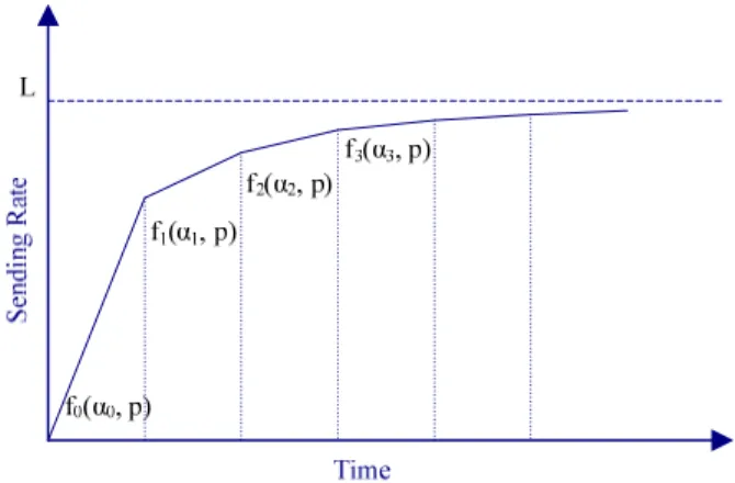
UDT adopts this efficiency idea and specifies a piecewise a(x) that is related to the link capacity. The fixed rate control interval of UDT is SYN, or the synchronization time interval, which is 0.01 second. UDT rate control is a special DAIMD algorithm by specifying a(x) as: SYN S x L Cx 1500 1 10 ) ( log( ( )) (3)
In formula (3), x has the unit of packets/second. L is the link capacity measured by bits/second. S is the UDT packet size (in terms of IP payload) in bytes. C(x) is a function that converts the unit of the current sending rate x from packets/second to bits/second (C(x) = x * S * 8). is a protocol parameter, which is 9 in the current protocol specification.
The factor of (1500/S) in function (3) is to balance the impact of flows with different packet sizes. UDT treats 1500 bytes as a standard packet size.
Table 1 gives an example on how UDT increases its sending rate under different situations. In this example, we assume all packets are in 1500 bytes.
Table 1: UDT increase parameter computation example. The first column represents the estimated available bandwidth and the second column represents the increase in packets per SYN. While the available bandwidth increases to the next scope of 10's integral power, the increase parameter also increases by 10 times. B = L - C (Mb/s) inc (packets/SYN) B 0.1 0.00067 0.1 < B 1 0.001 1 < B 10 0.01 10 < B 100 0.1 100 < B 1000 1 … …
The UDT congestion control described above is not enabled until the first NAK is received or the flow window has reached the maximum size. This is the slow start period of the UDT congestion control. During this time the inter-packet time is kept as zero. The initial flow window size is 2 and it is set to the number of acknowledged packets each time an ACK is received. The slow start only happens at the beginning of a UDT connection, and once the above congestion control scheme is enabled, it will not happen again.
Figure 5: Sending rate changes over time. This figure shows the sending rate of a single UDT flow changes over time. This is the situation when there is no non-congestion loss and no other flows in the system; otherwise there will be oscillations in the sending rate.
Figure 5 shows an illustration of the increase of data sending rate of a single UDT flow. At each stage k (k = 0, 1, 2,…), the equilibrium can be reached when
x
0
, or intuitively, when the increase is balanced off by the decrease. The sending rate at equilibrium of stage k is approximately [27]:2 9 10 3 * e k k p x (4)
where p is the loss rate, and e is a value such that 10e-1 < L 10e. Many characterizes of UDT can be further deduced using formula (4). One interesting example is TCP friendliness. By comparing (4) against the simple version of the TCP throughput model ( 1.5/p/RTT ) [48], we can reach a sufficient condition to guarantee that UDT is less aggressive than TCP:
6 / 108 2 2 L SYN RTT (5)
Condition (5) shows that UDT is very friendly to TCP in low BDP environments. In addition, RTT has more impact on TCP friendliness than bandwidth.
3.2
Bandwidth Estimation
UDT uses receiver-based packet pairs [2] to estimate the link capacity L. The UDT sender sends out a packet pair (by omitting the inter-packet waiting time) every 16 data packets. Other patterns of packet pair or train can also be used because at the receiver side, whether the incoming packets consist of a packet pair or train can be determined from their timestamp information. The receiver records the inter-arrival time of each packet pair or train and uses a median filter (more complex mechanisms can be found in [44, 50]) on them to compute link capacity. Suppose the median inter-arrival time is T and the average packet size in the measure period is S, then the link capacity can be estimated by
S/T.
There are two major concerns in using packet pairs to estimate link capacity. One is the impact of cross traffic [19]. The existence of cross traffic can cause the capacity be under estimated. The other concern is the NIC interrupt coalescence [52]. High speed NIC often has the functionality of interrupt coalescence to avoid too frequent interrupts. This can cause multiple packet arrivals to be notified by one single interrupt and hence the link capacity may be overestimated. This error can be eliminated by using the average inter-arrival time of multiple packet pairs.
Nevertheless, estimation error is inevitable at most cases. We have seen that UDT may overestimate the capacity when there is only one flow in the network, whereas it tends to underestimate the capacity when there are multiple flows. For a single flow, capacity estimation error only affects the convergence time. For multiple flows, it can also affect the fairness. (Note that if all flows have the same estimation error, they can still reach fairness.)
One of the important reasons to use a ceiling function in UDT's increase formula (3) is to reduce the impact of estimation errors. As a simple intuitive example, if two flows share one 100 Mb/s link, flow 1 measures the link capacity as 101 Mb/s and flow 2
measures it as 99 Mb/s, then the two flows will still share the bandwidth almost equally. After flow 1 exceeds 1 Mb/s, it will enter the same stage as flow 2, and both of the two flows will have the same increments and decrements.
3.3
Dealing with Packet Loss
While in most loss-based congestion control work, packet loss is regarded as a simple congestion indication, few of them have investigated the loss pattern in real networks. Because one single loss may cause a multiplicative rate decrease, dealing with packet loss is very important.
There are three particular kinds of situations related to packet loss that need to be addressed: loss synchronization, non-congestion loss, and packet reordering. Loss synchronization is a condition in which all concurrent flows experience packet loss at almost the same time. Non-congestion loss is usually caused by link error and can give transport protocols false signals of network congestion. Finally, packet reordering can mislead the receiver as packet losses.
In particular, there has been an effective approach for packet reordering [69], so in this subsection we only focus on the first two situations, for which the solutions in literatures do not apply to UDT.
3.3.1
Loss Synchronization
The phenomenon of "loss synchronization" or "global synchronization" is the situation when all concurrent flows increase and decrease their sending rate at the same time, thus the aggregate throughout has a very large oscillation and leads to low aggregate utilization of the bandwidth. This is due to the fact that almost all the flows will experience packet drops when congestion occurs and have to drop their sending; when there is no congestion, they all increase the sending rate.
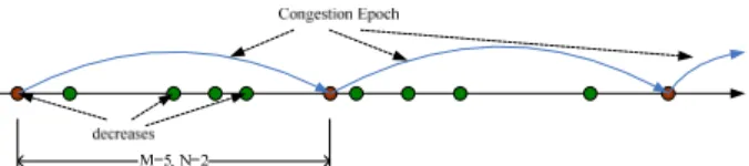
We use a randomization method to alleviate this problem. To describe this method, we define three terms. A loss event is the event when packet losses are detected. A UDT sender can detect a loss event when it receives a NAK report. A congestion event is a particular loss event when the largest sequence number of the lost packets in this loss event is greater than the largest sequence number that has been sent when the last rate decrease occurred. We call the period between two continuous congestion events a congestion epoch. Suppose there are M loss events between two continuous congestion events, and N is a random number that satisfies the uniform distribution between 1 and M.
For each congestion epoch, the decrease factor of the UDT control algorithm is randomized starting from 1/9 to [1 – (8/9)N]. Once a NAK is received, if this NAK starts a new congestion epoch, i.e., this is a congestion event, the packet-sending period is increased by 1/8 (which is equivalent to decreasing the sending rate by 1/9), and the packet sending is stopped for the next SYN time. For every N loss events, the packet sending period will be further increased by another 1/8.
Figure 6: De-synchronization of UDT control algorithm. The figure demonstrates the random loss decrease algorithm. In this figure, each node is a loss event on the time sequence, whereas a congestion epoch is noted as the period between the source and the sink of a directional arrow on the time sequence. In this example sequence, the first congestion epoch contains 5 loss events.
The process above can be described with the following algorithm. In this algorithm, LSD is the largest sequence number ever sent when the last NAK is received, STP is the packet sending period,
NumNAK and AvgNAK are two variables used to record the number of NAKs in the current congestion epoch and its smooth average value (the M value), and DR is the random number between 1 and AvgNAK (the N value).
Algorithm: Random Loss Decrease
1) If the largest lost sequence number in the NAK is greater than LSD:
a) Increase the STP by 1/8: STP = STP * (1 + 1/8).
b) Update AvgNAK: AvgNAK = (AvgNAK * 7 + NumNAK) / 8.
c) Update DR = rand(AvgNAK). d) Reset NumNAK = 0; e) Record LSD.
2) Otherwise, increase NumNAK by 1, and if NumNAK % DR = 0: a) Increase the STP by 1/8: STP = STP * (1 + 1/8).
b)
Record LSD.
Figure 7: Random loss-based decrease algorithm. Note that the use of explicit loss report (NAK) is different from the use of duplicate ACKs in TCP. With duplicate ACKs, the sender may not know all the loss events in one congestion event, and usually only the first loss event is detected. In fact, most TCP implementations will not drop the sending rate more than once in each RTT. However, in UDT, all loss events will be reported by NAK.
3.3.2
Noisy Link
Loss based control algorithms might not work well if there are significant non-congestion packet losses (e.g., due to link error, bad behavior of equipments, etc.), because they regard all packet losses as due to network congestion and will decrease the data sending rate accordingly. Although the link error rate on optical links is extremely small, sometimes there are non-congestion packets losses due to equipment problems and wrong configurations. We use a simple mechanism in UDT to tolerate such problems.
On noisy links, UDT does not react to the first packet loss in a congestion event. However, it will decrease the sending rate if there is more than one packet loss in one congestion event. This scheme is very effective in networks with small non-congestion
packet losses. Not surprisingly, it also works for light packet reordering problems.
This algorithm is equivalent to removing Step 1.a in the random loss decrease algorithm described in Figure 7.
4.
COMPOSABLE UDT
4.1
Overview
While UDT has been successful for bulk data transfer over high-speed networks, we feel that it could have benefited a much broader audience. We expanded UDT so that it can be easily configurable to satisfy more requirements for both network research and application development. We call this Composable UDT.
However, we emphasize here that this framework is not a replacement for, but a complement to the kernel space network stacks. General protocols like UDP, TCP, DCCP [41], and SCTP [58] should still exist inside the kernel space of operating systems, but OS vendors may be reluctant to support too many protocols and algorithms, especially those application specific or network specific ones.
Composable UDT supports a wide variety of control algorithms, including but not limited to, TCP algorithms (e.g., NewReno [24], Vegas [10], FAST [37], Westwood [25], HighSpeed [23], BiC [67], and Scalable [40]), bulk data transfer algorithms (e.g., SABUL [26], RBUDP [33], LambdaStream [66], CHEETAH [61], and Hurricane [65]), and group transport control algorithms (e.g., CM [4] and GTP [63]).
We envision the following use scenarios for Composable UDT: Implementation and deployment of new control algorithms. Certain control algorithms may not be appropriate to be deployed in kernel space, e.g., a bulk data transfer mechanism used only in private links. These algorithms can be implemented using Composable UDT.
Application awareness support and dynamic configuration. An application may choose different congestion control strategies under different networks, different users, and even different time slots. Composable UDT supports these application aware algorithms.
Evaluation of new control algorithms. Even if a control algorithm is to be deployed in kernel space, it needs to be tested thoroughly before OS vendors distribute the new version. It is much easier to test the new algorithms using Composable UDT than modifying an OS kernel.
4.2
The CCC Interface
We identify four categories of configuration features to support configurable congestion control mechanisms. They are 1) control event handler callbacks, 2) protocol behavior configuration, 3) packet extension, and 4) performance monitoring.
4.2.1
Control Event Callbacks
Seven basic callback functions are defined in the base CCC class. They are called by UDT when a control event is triggered. init and close: These two methods are called when a UDT connection is set up and when it is torn down. They can be used to initialize necessary data structures and release them later.
onACK: This handler is called when an ACK (acknowledgment) is received at the sender side. The sequence number of the acknowledged packet can be learned from the parameters of this method.
onLoss: This handler is called when the sender detects a packet loss event. The explicit loss information is given to users as the
onLoss interface parameters. Note that this method may be redundant for most TCP algorithms that use only duplicate ACKs to detect packet loss.
onTimeout: A timeout event can trigger the action defined by this handler. The timeout value can be assigned by users, otherwise it uses the default value according to the TCP RTO calculation described in RFC 2988 [51].
onPktSent: This is called right before a data packet is sent. The packet information (sequence number, timestamp, size, etc.) is available through the parameters of this method.
onPktReceived: This is called right after a data packet is received. Similar to onPktSent, the entire packet information can be accessed by users through the function parameters.
onPktSent and onPktReceived are the two most powerful event handlers, because they allow users to check every single data packet. For example, onPktReceived can be redefined to compute the loss rate in TFRC. Due to the same reason, these two callbacks can also allow users to trace the microscopic behavior of a protocol.
processCustomMsg: This method is used for UDT to process user-defined control messages.
4.2.2
Protocol Configuration
To accommodate certain control algorithms, some of the protocol behavior has to be customized. For example, a control algorithm may be sensitive to the way that data packets are acknowledged. Composable UDT provides necessary protocol configuration APIs for these purposes.
It allows users to define how to acknowledge received packets at the receiver side. The functions of setACKTimer and
setACKInterval determine how often an acknowledgment is sent, in elapsed time and the number of arrived packets, respectively. The method of sendCustomMsg sends out a user-defined control packet to the peer side of a UDT connection, where it is processed by callback functions processCustomMsg.
Finally, Composable UDT also allows users to modify the values of RTT and RTO. A new congestion control class can choose to use either the RTT value provided by UDT, or its own calculated value. Similarly, the RTO value can also be redefined.
4.2.3
Packet Extension
It is necessary to allow user-defined control packets for a configurable protocol stack.
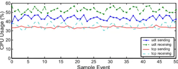
Because our Composable UDT library is mainly focused on congestion control algorithms, we only give limited customization ability to the control packets. Data packet processing contributes to a large portion of CPU utilization and customized data packets may hurt the performance.
Users can define their own control packets using the Extended Type information in the UDT control packet header (Figure 3). The detailed control information carried by these packets varies
depending on the packet types. At the receiver side, users need to override processCustomMsg to tell Composable UDT how to process these new types of packets.
4.2.4
Performance Monitoring
Protocol performance information supports the decisions and diagnosis of a control algorithm. For example, certain algorithms need some history information to tune the future packet-sending rate. Meanwhile, when testing new algorithms, performance statistics and internal protocol parameters are needed.
The performance monitor provides information including the duration time since the connection was started, RTT, sending rate, receiving rate, loss rate, packet sending period, congestion window size, flow window size, number of ACKs, and number of NAKs. UDT records these traces whenever the values are changed.
These performance traces can be read in three categories (when applicable): the aggregate values since the connection started, the local values since the last time the trace is queried, and the instant values when the query is made.
4.3
Expressiveness
To evaluate the expressiveness of Composable UDT, we implement a set of representative control algorithms using the library. Any algorithms belonging to a similar set can be implemented in a similar way. Meanwhile, we show that the implementation is simple and easy to learn.
In this section, we describe in detail how to implement control algorithms of rate based UDP, TCP variants, including both loss-based and delay-loss-based algorithms, and group transport protocols as well.
Composable UDT uses an object-oriented design. It provides a base C++ class (CCC) that contains all the functions and event handlers described in Section 4.2.1. A new control algorithm can inherit from this class and redefine certain control event handlers. The implementation of any control algorithm is to update at least one of the two control parameters: the congestion window size (m_dCWndSize) and the packet-sending period (m_dPacketPeriod), both of which are CCC class member variables.
4.3.1
Rate-based UDP
A rate-based reliable UDP library (CUDPBlast) is often used to transfer bulk data over private links. To implement this control mechanism, CUDPBlast initializes the congestion window with a very large value so that the window size will not limit the packet sending. The rest is to provide a method to assign a data transfer rate to a specific CUDPBlast instance. A piece of pseudo code is shown below:
class CUDPBlast: public CCC
{
public:
CUDPBlast() {m_dCWndSize = 83333.0;} void setRate(int mbps)
{
m_dPktSndPeriod = (SMSS * 8.0) / mbps; }
By using setsockopt an application can assign CUDPBlast to a UDT socket and by using getsockopt the application can obtain a pointer to the instance of CUDPBlast being used by the UDT socket. The application can then call the setRate method of this instance to set or modify a fixed sending rate at any time.
4.3.2
Standard TCP (TCP NewReno)
As a more complex example, we further show how to use the Composable UDT library to implement the standard TCP congestion control algorithm (CTCP). Because a large portion of newly proposed congestion control algorithms are TCP-based, this CTCP class can be further inherited and redefined to implement more TCP variants, which we will describe in the next two subsections.
TCP is a pure window-based control protocol. Therefore, during initialization, the inter-packet time is set to zero. In addition, TCP needs data packets to be acknowledged frequently, usually every one or two packets1. This is also configured in the initialization.
TCP does not need explicit loss notification, but uses three duplicate ACKs to indicate packet loss. Therefore, for congestion control, CTCP only redefined two event handlers: onACK and
onTimeout. In onACK, CTCP detects duplicate ACKs and takes proper actions. Here is the pseudo code of the fast retransmit and fast recovery algorithm in RFC 2581 [3]:
virtual void onACK(constint& ack) {
if (three duplicate ACK detected)
{
// ssthresh = max{flight_size / 2, 3} // cwnd = ssthresh + 3 * SMSS }
else if (further duplicate ACK detected) {
// cwnd = cwnd + SMSS }
else if (end fast recovery) { // cwnd = ssthresh } else { // cwnd = cwnd + 1/cwnd } }
The CTCP implementation can provide more TCP event handlers such as DupACKAction and ACKAction, which will further reduce the work of implementing new TCP variants.
Note that here we are only implementing TCP’s congestion control algorithm, but NOT the whole TCP protocol. The Composable UDT library does not implement exactly the same protocol mechanisms as in the TCP specification but it does provide similar functionality. For example, TCP uses byte-based
1 Although TCP uses accumulative acknowledgments, a TCP
implementation usually acknowledges at the boundary of a data segment. This is equivalent to acknowledging a UDT data packet in CTCP.
sequencing whereas UDT uses packet-based sequencing, but this should not prevent CTCP from simulating TCP’s congestion avoidance behavior.
4.3.3
New TCP Algorithms (Loss-based)
New TCP variants that use loss-based approaches usually redefine the increase and decrease formulas of the congestion window size. Implementations of these protocols can simply inherit from CTCP and redefine proper TCP event handlers.
For example, to implement Scalable TCP, we can simply derive a new class from CTCP, and override the actions of increasing (by 0.01 instead of 1/cwnd) and decreasing (by 1/8 instead of 1/2) the congestion window size.
Similarly, we have also implemented HighSpeed TCP (CHS), BiC TCP (CBiC), and TCP Westwood (CWestwood).
4.3.4
New TCP Algorithms (Delay-based)
Delay-based algorithms usually need accurate timing information for each packet. For efficiency, UDT does not calculate RTT for each data packet because it is unnecessary for most control algorithms. However, this can be done by overriding onPktSent
and onACK event handlers, where the time of packet sending and the arrival of its acknowledgment can be recorded. For algorithms preferring one-way delay (OWD) information, each UDT packets contains the sending time in its packet header, and a new algorithm can override onPktReceived to calculate OWD. Using the strategy described above, we implement the TCP Vegas (CVegas) control algorithm. CVegas uses its own data structure to record packet departure timestamps and ACK arrival timestamps, and then calculates accurate RTT values. With simple modifications to the control formulas, we further implement FAST TCP (CFAST).
4.3.5
Group Transport Control
While we have demonstrated that Composable UDT can be used to implement end-to-end unicast congestion control algorithms, we now show that it can also be used to implement group-based control mechanisms, such as CM and GTP.
To support this feature, the new algorithm class simply needs to implement a central manager to control a group of connections. The control parameters are calculated by the central manager and then fed back to the control class instance of each individual connection.
We implemented GTP (CGTP) as an example of group-based control mechanisms. The GTP protocol controls a group of flows with the same destination. CGTP tunes the packet-sending rate at the receiver side periodically and feeds back the parameters using Composable UDT’s sendCustomMsg method.
4.3.6
Summary
We have implemented nine example algorithms using Composable UDT, including rate-based reliable UDP, TCP and its variants, and group-based protocols. We demonstrated that our Composable UDT library can support a large variety of congestion control algorithms, which are supported by only 8 event handlers, 4 protocol control functions, and 1 performance monitoring function.
The concise Composable UDT API is easy to learn. In fact, it takes a small piece of code to implement most of the algorithms described above. Table 2 lists the lines of code (LOC) of
implementations of TCP algorithms using Composable UDT, as well as the LOC of those native implementations (Linux kernel patches). The LOC value is estimated by the number of semicolons in the corresponding C/C++ code segment.
To give more insight into the difference between LOCs in Composable UDT based implementations and native implementations, we use the FAST TCP case as an example. The 31 lines of CFAST only implement the FAST congestion avoidance algorithm, whereas much of its code, especially the timing part, is inherited from CVegas. In contrast, of the 367 lines of FAST TCP patch, 142 of them are used to implement the FAST protocol (new files), 81 lines are used to modify the Linux TCP files, 86 lines are used to do monitoring and statistics, and 58 lines are used to do burst control and pacing.
As a reference point, the UDT library has 3134 lines of effective code (i.e., excluding comments, blank lines, etc.), SABUL has 2670 lines of code, and the RBUDP library has approximately 2330 lines of code. While these numbers are not enough to reflect the complexity of implementing a transport protocol, the much smaller number of LOC values of Composable UDT based implementation can indicate the simplicity.
Table 2. Lines of code (LOC) of implementations of TCP algorithms. This table lists LOC of different TCP algorithms implemented using Composable UDT and their respective Linux kernel patches (native implementations). The LOC of Linux patches include both added lines and removed lines.
Native
Protocol Composable UDT
Added Removed TCP 28 - Scalable TCP 11 192 29 HighSpeed TCP 8 27 1 BiC TCP 38 248 30 TCP Westwood 27 145 2 TCP Vegas 37 + 362 132 6 FAST TCP 31 365 2
To give more insight into the difference between LOCs in Composable UDT based implementations and native implementations, we use the FAST TCP case as an example. The 31 lines of CFAST only implement the FAST congestion avoidance algorithm, whereas much of its codes, especially the timing part, are inherited from CVegas. In contrast, of the 367 lines of FAST TCP patch, 142 of them are used to implement the FAST protocol (new files), 81 lines are used to modify the Linux TCP files, 86 lines are used to do monitoring and statistics, and 58 lines are used to do burst control and pacing.
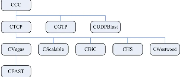
The class inheritance relationship of these Composable UDT implemented algorithms can be found in Figure 8. Code reuse by class inheritance also contributes to the small LOC values of those TCP-based algorithms.
2 CVegas reuses a timing class implemented by UDT, which
contains 36 lines of code.
CCC
CTCP CGTP CUDPBlast
CScalable CBiC CHS CWestwood
CVegas
CFAST
Figure 8: Composable UDT based protocols. This figure shows the class inheritance relationship among the control algorithms we implemented. Note that this is only for the purpose of code reuse, and it does NOT imply any other relationship among these algorithms.
4.4
Similarity
In most cases, congestion/flow control algorithms are the most significant factor that determines a protocol’s performance-related behavior (throughput, fairness, and stability). Less significant factors include other protocol control mechanisms, such as RTT calculation, timeout calculation, acknowledgment interval, etc. We have made most of these control mechanisms configurable through the CCC interface and the UDT protocol control interface. In this subsection we will show that a Composable UDT based implementation demonstrates similar performance to a native implementation.
Since TCP is probably the most representative control protocol, we compared an application level TCP implementation using our Composable UDT library (CTCP) against the standard TCP implementation provided by Linux kernel 2.4.18.
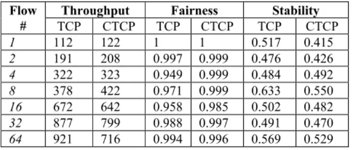
The experiment was performed between two Linux boxes between Chicago and Amsterdam. The link is 1 Gb/s with 110 ms RTT and was reserved for our experiment only in order to eliminate cross traffic noises. Each Linux box has dual Xeon 2.4GHz processors and was installed with Linux kernel 2.4.18. We started multiple TCP and CTCP flows in separate runs, each of which was kept running for at least 60 minutes. The total TCP buffer size was set to at least the size of BDP (bandwidth delay product). Both TCP and CTCP experiments used the same testing program (except the connections were TCP and CTCP, respectively) with the same configuration (buffer size, etc.). We recorded the aggregate throughput (value between 0 and 1000 Mbps), fairness index (value between 0 and 1), and stability index (equal to or greater than 0) in Table 3. The definitions of the fairness index and stability index can be found in Section 5. The fairness index represents how fairly the bandwidth is shared by concurrent flows and larger values are better. The stability index describes the oscillations of the flows and smaller values mean less oscillation. These three measurements summarize most of the performance characteristics of a congestion control algorithm. From Table 3, we find that TCP and CTCP have pretty similar throughput for small numbers of parallel flows. However, as the number of parallelism increases, CTCP stops increasing its throughput first and thus has a significantly smaller throughput
than TCP when there are 64 parallel flows3. Further analysis
indicates that the reason for this is that CTCP costs more CPU than kernel implemented TCP and with 64 flows the CPU time has been used up. To verify this assertion, we started another experiment using machines with dual AMD 64-bit Opteron processors and this time CTCP reaches more than 900Mbps at 64 parallel flows.
Table 3: Performance characteristics of TCP and CTCP with various parallel flows. The table lists the aggregate throughput (in Mb/s), fairness index, and stability index of concurrent TCP and CTCP flows. Each row records an independent run with a different number of parallel flows.
Throughput Fairness Stability
Flow # TCP CTCP TCP CTCP TCP CTCP 1 112 122 1 1 0.517 0.415 2 191 208 0.997 0.999 0.476 0.426 4 322 323 0.949 0.999 0.484 0.492 8 378 422 0.971 0.999 0.633 0.550 16 672 642 0.958 0.985 0.502 0.482 32 877 799 0.988 0.997 0.491 0.470 64 921 716 0.994 0.996 0.569 0.529
In spite of the CPU utilization limitation, both of the implementations have similar performance on fairness and stability. They both realize good fairness with near-one fairness indexes, as the AIMD algorithm indicates. The stability indexes are around 0.5 for all runs.
In addition to the experiments above, we have also tested several reliable UDP-based protocols such as UDP Blast (CUDPBlast) to examine if the Composable UDT based implementation conforms to the protocol’s theoretical performance. We also examined the performance of Composable UDT in a real streaming merge application, in which the receiver (where data is merged) requests an explicit sending rate to the data sources. This service is provided by a specific control mechanism implemented using Composable UDT. The results of these experiments were positive and expected performance was reached.
5.
PERFORMANCE EVALUATION
In this section, we evaluate UDT’s performance using several experiments on real high-speed networks. While we have also done extensive simulations covering the majority of network situations, we choose real world experiments here because they give us more insight into UDT's performance.
We use TCP as the baseline to compare against UDT. While there are many new protocols and congestion control algorithms, it is hard to choose a mature one as the baseline; complete comparison of all these protocols is a relative complicated work and is beyond of the scope of this paper. In fact, there has been work to compare some of these protocols [5, 7, 32, 42, 43]. In particular, a rather complete experimental comparison on new TCP variants can be found in [32].
3 TCP throughput will also start to decrease as the number of
parallel flows increases [56].
5.1
Evaluation Strategy
The performance characteristics to be examined include efficiency (throughput), intra-protocol fairness, TCP friendliness, and stability. We will also evaluate the implementation efficiency (CPU usage).
Efficiency (Throughput). We define the efficiency of UDT as the aggregate throughput of all concurrent UDT flows. Efficiency is one of the major motivations of UDT, which is supposed to utilize the high bandwidth efficiently, that is, utilize as much bandwidth as possible. Particularly, in grid computing, there are usually only a small number of bulk data flows sharing the network. A single UDT flow should reach high efficiency as well. Suppose there are m UDT flows in the network and the i-th flow has an average throughout of xi, the efficiency index is defined as
m i i x E 1
Intra-protocol Fairness. The fairness characteristic measures how fairly the concurrent UDT flows share the bandwidth. The most frequently used fairness rule is the max-min fairness, which maximizes the throughput of the poorest flows. If there is only one bottleneck in the system, then all the concurrent flows should share the bandwidth equally according to the max-min rule. In this case, we can use Jain’s fairness index [35] to quantitatively measure the fairness characteristics of a transport protocol.
n i i n i i n x x F 1 2 2 1
where n is the number of concurrent flows and xi is the average throughput of the i-th flow. F is always less than or equal to 1. A larger value of F means better fairness, and F = 1 is the best, which means all flows have equivalent throughput.
TCP Friendliness. TCP friendliness is rather a more obscure measurement than the others, because it is almost impossible for a protocol with different control algorithms to reach the same performance as TCP's and it is not reasonable to limit the throughput of a new protocol in high BDP environments to the throughput of TCP while the latter is very inefficient.
We consider the TCP friendliness separately in different situations, which are related to two factors: the network BDP and the TCP flow lifetime. First, in low BDP environments, where TCP can utilize the bandwidth efficiently, we expect that UDT should at least share the bandwidth with TCP fairly (equally); in high BDP environments, where TCP cannot efficiently use the bandwidth, we expect UDT to make use of the bandwidth that TCP fails to use but leave enough space for TCP to increase. Second, TCP's behavior can be very different for bulk flows and Short-lived flows (considering the impact of TCP slow start at the beginning of a connection). We consider the situation of short-lived TCP separately because a majority of TCP traffic over the Internet are short-lived flows (e.g., web traffic).
For bulk TCP flows, suppose there are m UDT and n TCP flows coexisting in the network. With the same network configuration, we start m+n TCP flows separately. The average throughput for the i-th TCP flow in each run is xiandyi, respectively. We define the TCP friendliness index as:
n m i i n i i y n m x n T 1 1 1 1
where the denominator is the fair share of TCP.
T = 1 is the ideal friendliness; T > 1 means UDT is too friendly; and T < 1 means UDT overruns TCP.
For short-lived flows, we will compare the aggregate throughput of a large number of small TCP flows under different numbers of background bulk UDT flows.
Stability (Oscillations). We use the term of “stability” in this section to describe the oscillation characteristic of a data flow. A smooth flow is regarded as desirable behavior for most situations, and it often (although not necessarily) leads to better throughput. Note that this is different from the meaning of “stable” in control theory, and the latter means the convergence to a unique equilibrium from any start point.
To measure oscillations, we have to consider the average throughput in each unit time interval (a sample). We use standard deviation of the sample values of the throughput of each flow to express its oscillation [37]:
n i m k i i i x k x m x n S 1 1 2 ) ( 1 1 1 1
where n is the number of concurrent flows; m is the number of throughput samples for each flow; xi(k) is the k-th sample value of
flow i; and
x
iis the average throughput of flow i.CPU Usage. CPU usage is usually measured by the usage percentage. Note that CPU percentage is system dependable. These values are only comparable against those values obtained on the same system, or at least systems with the same configuration.
5.2
Efficiency, Fairness, and Stability
We performed two groups of experiments in different network settings to examine UDT’s efficiency, intra-protocol fairness, and stability property.
5.2.1
Case Study 1
In the first group of experiments, we start three UDT flows from a StarLight node to another StarLight local node, a node in Canarie (Ottawa, Canada), and a node in SARA (Amsterdam, the Netherlands), respectively (Figure 9). All nodes have a 1Gb/s NIC and dual Xeon CPU and are installed with Linux 2.4.
Figure 10 shows the throughout of the single UDT flow over each link when the three flows are started separately. A single UDT flow can reach about 940Mbps over 1Gbps link with both 40us short RTT and 110ms long RTT. It can reach about 580Mbps over an OC-12 link with 15.9ms RTT between Canarie and StarLight. In contrast, TCP only reaches about 128 Mb/s from Chicago to Amsterdam after a thorough tuning for performance.
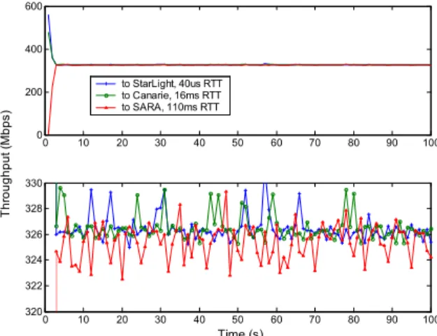
Figure 11 shows the throughput when the three flows were started at the same time. This experiment demonstrates the fairness property among UDT flows with different bottleneck bandwidths and RTTs. All the three flows reach about 325 Mb/s. Using the same configuration, TCP’s throughputs are 754 Mb/s (to
Chicago), 151 Mb/s (to Canarie), and 27 Mb/s (to Amsterdam), respectively. 1 Gb/s RTT = 110 ms Chicago Ottawa Amsterdam Chicago RTT = 40us1 Gb/s
Figure 9: Experiment network configuration. This figure shows the network configuration connecting our machines used for testing at Chicago, Ottawa, and Amsterdam. Between any two local Chicago machines the RTT is about 40us and the bottleneck capacity is 1Gb/s. Between any two machines at Chicago and Amsterdam respectively the RTT is 110ms and the bottleneck capacity is 1Gb/s. Between any two machines at Chicago and Ottawa respectively the RTT is 16ms and the bottleneck capacity is 622Mb/s. Amsterdam and Ottawa are connected via Chicago. The total bandwidth connecting the Chicago cluster is 1Gb/s.
0 10 20 30 40 50 60 70 80 90 100 0 200 400 600 800 1000 Time (s) Thr oughput ( M bps) to Chicago, 1Gbps, 0.04ms to Canarie, OC-12, 16ms to Amsterdam, 1Gbps, 110ms
Figure 10: UDT performance over real high-speed network testbeds. This figure shows the throughput of a single UDT flow over three different links described in Figure 4-17. The three flows are started separately and there is no other traffic during the experiment. 0 10 20 30 40 50 60 70 80 90 100 0 200 400 600 0 10 20 30 40 50 60 70 80 90 100 320 322 324 326 328 330 Time (s) Th roug hpu t ( M bp s) to StarLight, 40us RTT to Canarie, 16ms RTT to SARA, 110ms RTT
Figure 11: UDT fairness in real networks. This figure shows the throughputs of 3 concurrent UDT flows over the different links described in Figure 10. No other traffic exists during the experiment. The figure below is a local expansion of the sub-figure above.
5.2.2
Case Study 2
We set up another experiment to check the efficiency, fairness, and stability performance of UDT at the same time. The network configuration is shown in Figure 12. Two sites, StarLight (Chicago) and SARA (Amsterdam), are connected with 1 Gb/s link. At each site, four nodes are connected to the gateway switch through 1GigE NIC. The RTT between the two sites is 104ms. All nodes run Linux 2.4.19 SMP on machines with dual Intel Xeon 2.4GHz CPUs.
Figure 12: Fairness testing configuration. This figure shows the network topology used in UDT experiments. Four pairs of nodes share 1 Gb/s, 104 ms RTT link connecting two clusters at Chicago and Amsterdam, respectively.
For the four pairs of nodes, we start a UDT flow every 100 seconds, and stop each of them in the reverse order every 100 seconds, as depicted in Figure 13.
Figure 13: Flow start and stop configuration. This figure shows the UDT flow start/termination sequence in an experiment configuration. There are 4 UDT flows and each flow is started every 100 seconds, and stopped in the reverse order every 100 seconds. The lifetime of each flow is 100, 300, 500, and 700 seconds, respectively. 0 100 200 300 400 500 600 700 0 200 300 450 900 1000 Time (s) Th ro ug ho ut (M b its /s )
Figure 14: UDT efficiency and fairness. This figure shows the throughput of the 4 UDT flows in Figure 13 over the network in Figure 12. The highest line is the aggregate throughput.
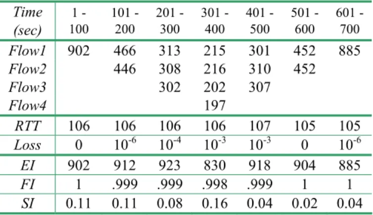
The results are shown in Figure 14 and Table 4. Figure 14 shows the detailed performance of each flow and the aggregate throughput. Table 4 lists the average throughput of each flow, the average RTT and loss rate at each stage, the efficiency index (EI), the fairness index (FI), and the stability index (SI).
All stages achieve good bandwidth utilization. The maximum possible bandwidth is about 940 Mb/s on the link, measured by other benchmark software. The fairness among concurrent UDT flows is very close to 1. The stability index values are very small, which means the sending rate is very stable (few oscillations). Furthermore, UDT causes little increase in the RTT (107 ms vs. 104 ms) and a very small loss rate (no more than 0.1%).
Table 4: Concurrent UDT flow experiment results. This table lists the per-flow throughput, end-to-end experienced RTT, overall loss rate, the efficiency index, the fairness index, and the stability index of the experiment of Figure 14.
Time
(sec)
1 - 100 101 - 200 201 - 300 301 - 400 401 - 500 501 - 600 601 - 700Flow1
902
466
313
215
301
452
885
Flow2
446
308
216
310
452
Flow3
302
202
307
Flow4
197
RTT
106
106
106
106
107
105
105
Loss
0
10
-610
-410
-310
-30
10
-6EI
902
912
923
830
918
904
885
FI
1
.999 .999 .998 .999
1
1
SI
0.11 0.11 0.08 0.16 0.04 0.02 0.04
5.3
TCP Friendliness
Short-lived TCP flows such as web traffic and certain control messages comprise a substantial part of Internet data traffic. To examine the TCP friendliness property against such TCP flows, we set up 500 TCP connections where each transfers 1MB of data from Chicago to Amsterdam; a varying number of bulk UDT flows were started as background traffic when the TCP flows are started. TCP's throughput should decrease slowly as the number of UDT flows increases. The results are shown in Figure 15. They decrease from 69 Mb/s (without concurrent UDT flows) to 48 Mb/s (with 10 UDT concurrent flows).
0 1 2 3 4 5 6 7 8 9 10 20 30 40 50 60 70 80
Number of UDT flows
TC P Th ro ug hp ut (M b ps )
Figure 15: Aggregate throughput of 500 small TCP flows with different numbers of background UDT flows. This figure shows the aggregate throughput of 500 small TCP transactions (each transferring 1MB data), under different numbers of background UDT flows varying from 0 to 10.