Electric Energy and Potential

J. Newman, Physics of the Life Sciences, DOI: 10.1007/978-0-387-77259-2_15, © Springer Science+Business Media, LLC 2008

EL E C T R I C PO T E N T I A L EN E R G Y 3 7 3

In the last chapter we discussed the forces acting between electric charges. Electric fields were shown to be produced by all charges and electrical interactions between charges were shown to be mediated by these electric fields. As we’ve seen in our study of mechanics, conservation of energy principles can often be used to under-stand the interactions and dynamics of a system. In this chapter we introduce the concept of electric potential energy and electric potential, and apply these consid-erations to a variety of situations. The fundamental electric interactions in atomic, macroscopic, and macromolecular systems are each presented. Biological mem-branes are discussed in some detail, with emphasis on their ability to act as capac-itors, energy storage devices. Membrane channels are introduced, focusing on sodium channels: how they work and how they are selective. We return to a more detailed description of the electrical properties of channels in the next chapter. This chapter concludes with a discussion of the mapping of the electric potential pro-duced by various organs of the human body including muscles, heart, and brain (EMG, EKG, and EEG, respectively). These medical techniques are often used for diagnostic purposes.

1. ELECTRIC POTENTIAL ENERGY

The electric force is a conservative force. As we saw in Chapter 4, this means that the work done by the electric force in moving a particle (in this case, charged) between two points is independent of the path and depends only on the starting and ending locations. Furthermore, there is an electric potential energy function that we can write down, whose negative difference at those two locations is equal to the work done by the electrical forces

(15.1) Recall that two expressions we have used for potential energy functions in mechanics, gravitational (mgy) and spring potential energy followed from the general definition of work and the particular form of the force. In a similar way, if Coulomb’s law for the force due to a point charge q₁, on a second point charge q₂, separated by a distance r is substituted into the general definition of work (see the box below), one obtains the electric potential energy of the two point charges (15.2) PE_E (r)⫽ q1q2 4pe₀ r. 11 2kx22, ⫺(PE_E,final⫺PE_E,inital )⫽- ¢PE

E⫽W.

15

Note that, just as in the mechanical energy cases, we need to define the location of zero potential energy because only potential energy differ-ences have meaning. For springs, the natural choice was to reference the spring potential energy to a zero value for an unstretched spring that exerts no force. For gravitational potential energy near the Earth’s surface, we were free to define the location of zero potential as we chose because the gravitational force on a mass is constant in the approximation we used. For other more general situations using gravity, the zero of gravitational potential energy occurs when all masses are infinitely far apart so as not to be interacting. Similarly, in the case of electrical forces, when the charges are infinitely far apart (r→⬁) they do not interact and it is there-fore natural to choose this situation to correspond to zero electric poten-tial energy. Equation (15.2) already satisfies this convention.

The electric potential energy for charges of like sign that repel one another is positive according to Equation (15.2), whereas for unlike charges that attract each other it is negative. Example plots for both cases are given in Figure 15.1. We recall that the negative of the slope of such a plot is equal to the force acting at position r. In this case, with one charge at the origin and the other at r, when PE_E(r)⬎0 because the energy decreases with increasing r, the negative of the slope is always positive, consistent with a repulsive force acting. The steeper the curve is, the larger the force (and therefore acceleration) acting. We can imagine a charged particle sit-ting on the energy curve and falling down its hill with a decreasing accel-eration (but still increasing velocity) as it moves toward larger r values. A charge projected toward the origin with some initial kinetic energy will travel up the PE_E hill as far as corresponds to the conversion of all its kinetic energy to potential before falling back down the energy hill.

Similarly, when PE_E(r)⬍0, because increasing r leads to less neg-ative, or increasing PE_E, the negative of the slope is itself negative, con-firming that the force is attractive. A charged particle placed on this curve will also fall down the potential hill ever more rapidly (with increasing acceleration) as its distance from the other charge at the ori-gin decreases. We discuss electric potential energies for other situations later in this chapter in connection with molecular bonding.

Having found an expression for the electric potential energy of a pair of point charges, we can write an expression for the total energy of this two-particle system. We include the kinetic energy of each particle, the electric potential energy, and any other mechanical potential ener-gies, PE_mech, appropriate to the situation. The conservation of energy principle then states that

(15.3)

As we have seen in applications in mechanics, energy conservation is a powerful concept that has a great degree of practical utility as well.

E⫽KE₁⫹KE₂⫹PE_mech⫹ q1 q2

4pe_o r⫽constant. Here we derive an expression for the electric

potential energy between two point charges. We imagine that there is a point charge, say

q₁⬎0, located at the origin and bring a sec-ond point charge, q₂⬎0, from infinitely far away where it does not feel any electric force to some distance r away from q₁. Because both charges are positive, there is a repulsive force between them and positive external work must be done to bring q₂ toward the charge at the origin. This work is equal and opposite to the (then, negative) work done on

q₂by the electric force from q₁. According to Equation (15.1) the change in potential energy will then be positive as might be expected, because if the external force is removed, the repulsive force will change the positive elec-tric potential energy of q₂into kinetic energy as it accelerates away from the origin.

From the general definition of work and Equation (15.1), the electric potential energy change is given by

where F is the electric force on charge q₂ and ␪is the angle between the force vector and the displacement vector The path taken by the charge does not matter, there-fore we choose it to be inward along the radial direction. In this case ␪ is equal to 180°, so that cos ␪is equal to ⫺1, and the displacement ds is equal to ⫺dr. We substi-tute Coulomb’s law for the force to find

Remembering that

we do the integration and evaluate the resulting expression at the limits to find that the potential energy at a distance r from the origin is given by Equation (15.2).

L 1 r2dr⫽ ⫺1 r , ¢PE⫽ ⫺q₁ q₂ 4pe_o L r q 1 r2dr. d s: . ¢PE⫽PE(r)⫺PE(q)⫽ -L r q [Fcosu]ds –4 –3 –2 –1 0 1 2 3 4 0 0.2 0.4 0.6 0.8 r (m) PE (J)

FIGURE 15.1Electric potential energy for two point charges of 1␮C magnitude with the upper curve for like sign charges and the lower curve for opposite charges.

EL E C T R I C PO T E N T I A L 3 7 5

Example 15.1Find an expression for the total energy of a hydrogen atom

treat-ing the electron as traveltreat-ing in a circular orbit around the stationary proton. Find an answer in terms of only the radius of the circular orbit.

Solution:The total energy consists of the kinetic energy of the electron,

travel-ing in a circle, and the electric potential energy of the electron–proton pair. We can write this as

To express the velocity of the electron in terms of its orbital radius, we use the fact that the only force on the electron is the Coulomb force and this must supply the centripetal acceleration according to

where both the force and centripetal acceleration are radially directed. Solving for mv2_{and substituting into the expression for the energy, we have}

This result says that the energy of a hydrogen atom is solely determined by the radius at which the electron orbits the proton. Note that the total energy is neg-ative. This is the signature of a bound system, with the negative potential energy term dominating over the positive kinetic energy term. We show in Chapter 25 that although this is a correct statement, the electron cannot orbit the proton at any radius, but only at certain allowed radii. This fact of nature leads to a dis-crete set of allowed energy levels for the hydrogen atom from the above equa-tion relating E to r, as first derived by Neils Bohr in 1913.

E⫽ 1 2 1 4pe_o e2 r ⫺ 1 4pe_o e2 r ⫽ ⫺ 1 8pe_o e2 r. F⫽ 1 4pe_o e2 r2⫽m v2 r , E⫽1 2 mv 2_⫹ 1 4pe₀ (⫹e)(⫺e) r .

In our discussion, electric potential energy has been introduced as arising from a direct interaction between charges via the Coulomb force. However, as was discussed in the last chapter, charges experience electric forces by direct interaction with an electric field due to the other charges rather than by action at a distance interactions of charges. In the next section, we introduce the electric potential, an important con-cept that intrinsically accounts for electric fields.

2. ELECTRIC POTENTIAL

A charged particle q_o in an electric field will experience a force equal to Associated with the interaction of the charge and the electric field is an electric potential energy. In the last section we saw the form of this potential energy if there is only one other point charge producing the electric field. In general, the electric potential energy will factor into a product of the charge q_o and a function that depends only on the other charges present and their distribution in space. This func-tion therefore represents the electric potential energy per unit charge and is called the

electric potential (or simply the potential), V(r), where

(15.4) Specifically, q_ois the charge located at the position at which the potential is being determined. The SI unit for electric potential is the volt, from Equation (15.4) given by

V(r)⫽PE_E (r)/q_o. q_oE : . E :

1 J/C⫽1 volt (V). From our discussion you may correctly suspect that V(r) is intimately related to the electric field produced by the other charges of the system; we show this con-nection shortly.

A very important unit for electric potential energy is the electron volt (eV), defined as the work done in moving an electronic charge through a potential difference of 1 V. From the charge on an electron, e⫽1.6⫻10⫺19C, we see that 1 eV⫽(1.6⫻ 10⫺19C)⫻(1 V)⫽1.6⫻10⫺19J. The electron volt is a very useful unit of energy in dealing with elementary particles such as electrons and protons since typical values are eV and awkward powers of 10⫺19are not needed.

To find an equation for the electric potential produced by a single point charge at the origin we can use Equation (15.2) in which we arbitrarily assign q₂ to be the charge located at the origin, and q₁ to be a charge q₀at an observation point a dis-tance r away where we wish to evaluate V. Using Equation (15.4), V is found by dividing Equation (15.2) by the charge q₁(⫽q₀). Because the label q₂is arbitrary, we drop its subscript to find a general expression for the electric potential of a point charge located at the origin,

(15.5) The electric potential function of a point charge maps the potential energy per unit charge in space, so that if a charge q₀ were placed at position r the potential energy of the two-charge system would be PE⫽q₀V(r). Implicit in this is the

zero-level of electric potential to be at infinite separation.

Note that the electric potential function of a point charge is defined everywhere in space and does not actually require another charge to interact with at a point in order to have a defined value at that point. Note the physical significance of the electric

potential at a point is the external work needed to move a unit positive charge from infinitely far away to that point along any path. This is true because the change

in electric potential energy equals the negative of the work done by the electric forces, which in turn is equal and opposite to the work done by external forces. So, for example, when you turn on your flashlight using two 1.5 V (2⫻1.5⫽3 V total) batteries, each unit of charge (1 C) that moves through the light bulb from one side of the battery to the other has used 3 J worth of battery energy.

It may be helpful to discuss an analogy with gravitation in order to better appreciate the meaning of electric potential. If a gravitational potential function had been analo-gously defined as PE_grav/m⫽gh, we see that such a “gravitational potential” would

cor-respond to the height function multiplied by the constant g. A roller coaster track would define this gravitational potential function by virtue of its height (Figure 15.2). An expres-sion for the gravitational potential energy function of someone riding on the roller coaster could then be easily found by multiplying that function by her mass. We did not introduce such a gravitational potential previously because, in our constant g approximation near the Earth’s surface, there would be no particular benefit. However, in the case of electricity with both positive and negative charges and with a spa-tially varying electric field, a mapping of the electric potential in space without regard for other interacting charges will be quite useful in the same way in which a mapping of the electric field was in the last chap-ter. Remember, however, that the electric potential is a scalar function, whereas the electric field is a vector quantity representing three func-tions, one for each vector component. A two-dimensional mapping of the scalar field representing the electric potential is similar to a topological map as discussed in the last chapter. In this case the height above a point in the plane represents the potential at that point. For the three-dimensional case, a scalar potential value is assigned to each point in space. These mappings can be visualized using color-coded computer methods, for example (see ahead to Figure 15.9). But, what is the rela-tion between the electric field and the electric potential?

V(r)⫽ q

4pe₀ r.

FIGURE 15.2Boomerang, Knott’s Berry Farm, California: gravitational potential varies with height.

To answer this question let’s take the simple case of a constant, uniform elec-tric field along the x-direction, reducing the problem to essentially one dimension. The force on a point charge q_oin such an electric field is and the work done on q_oby the electric field in moving a distance ⌬x along

the electric field direction is

Accordingly, the change in electric potential energy is so that the electric potential is given, in this simple case, by

(15.6)

where ⌬x is positive when along the E field direction. This equation relates the constant

electric field to the change in potential between two locations separated by⌬x. If the

potential function is known, then the electric field may be found from the relation (15.7)

where, in more than one dimension, there are similar expressions for the y and z com-ponents of the electric field. We mention that in the two- or three-dimensional case, given a mapping of the potential, the direction of the electric field is along the direc-tion of the steepest descent of the funcdirec-tion; that is, at any given point the electric field will be along that direction corresponding to the most rapid decrease in potential.

It is also worth mentioning that Equation (15.7) shows that the electric field may be expressed in units of (V/m) in addition to the previously introduced equivalent units of (N/C), with 1 N/C⫽1 V/m. The V/m is probably the more common unit for electric fields. Note that when Equation (15.7) is multiplied by a charge q_oits meaning becomes

(15.8) recovering an equation we have seen previously (Equation (4.23)).

For a positive electric charge q_o, the positive work done by an electric field acting alone will tend to drive the charge toward lower electric potential. This is seen by the fact that the product of W⫽F_x⌬x⫽q_oE_x⌬x⫽ ⫺q_o⌬V⬎0, so that ⌬V⬍0, and the charge will move down the potential hill. On the other hand, a negative charge will be attracted toward a higher potential because in that case with q_o⬍0 we must have ⌬V⬎0. Plots of electric potential have the same dependence on r as electric potential energy and are therefore quite similar to those in Figure 15.1. These statements concerning the directions of the forces acting on charges are gen-erally true despite our assumption of a constant electric field. Positive charges

tend to move toward lower potentials, or down potential hills, whereas nega-tive charges tend to move toward higher potentials, or up potential hills.

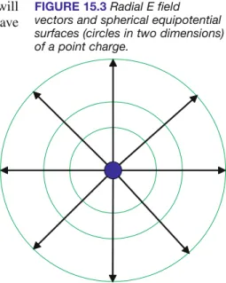
Figure 15.3 shows a mapping of the electric field and electric potential of a point charge. Note that the potential is mapped as a series of, in this case spheri-cal, contours of constant potential, known as equipotential surfaces (in three-dimensional space). No work is required to move a charge around on an equipotential surface because there is zero potential difference between all its points. Therefore, the electric field is always perpendicular to equipotential sur-faces, as we saw in the previous chapter for the case of a conducting surface. This is true because if the electric field had a component parallel to an equipotential surface, there would then be a net force acting to do work on a charge moving on the surface and it could not have a constant potential. It is straightforward to map

F_x⫽ ⫺ ¢PE E ¢x , E_x⫽ ⫺¢V ¢x , ¢V⫽ ¢PE E q_o ⫽⫺Ex¢x (uniform E), ¢PE E⫽⫺qo Ex¢x W⫽F¢x⫽q o Ex¢x. Fn⫽q_oEn EL E C T R I C PO T E N T I A L 3 7 7

FIGURE 15.3Radial E field vectors and spherical equipotential surfaces (circles in two dimensions) of a point charge.

equipotential surfaces once a mapping of the electric field is known. A surface is constructed that is everywhere perpendicular to the electric field lines (Figure 15.4).

An interesting example of an electrostatic potential in biology involves the honeybee. Coated with a fine layer of hair, the honeybee develops electrostatic charge when it flies, so that it actually can reach electrostatic potentials of several hundred volts. When the bee lands on a flower to drink nectar, pollen grains are electrostatically attracted to the fine hairs and will “jump” short distances through air from the electrostatic forces (see Figure 15.5). The honeybee then grooms itself and collects the adhered pollen in pollen sacs attached to its hind legs. Fortunately, not all of the pollen is collected for the bees to eat and the remaining pollen is able to pollinate other flowers as the bee visits them. It is also thought that the electrostatic voltage developed may help deliver pollen grains to the stigma of flowers by electrostatic attraction. (As an aside, for your information, recently there has been a precipitous decline in honeybee populations around the world. As yet the cause is unknown, although quite a number of factors have been surmised including virus infections, parasites, pesticide effects, nutritional issues, and other factors. Because hon-eybees pollinate about 90% of the fruit and vegetable crops in the United States alone, their declining numbers are having a major impact on the worldwide economy.)

3. ELECTRIC DIPOLES AND CHARGE

DISTRIBUTIONS

From the equation for the electric potential of a point charge (Equation (15.5)), we can find the electric potential of an arbitrary distribution of electric charge by generalization. If there are a number of individual point charges in the system (see Figure 15.6), the potential at some point in space, that we call the observation point, is simply the algebraic sum of the individual potentials due to each charge,

(15.9) where r_iis the distance from the observation point to the ith charge, q_i. In this sum, one must be careful to include the sign of the electric charge. There is a clear advantage in calculating the net electric potential, a scalar quantity, over adding vector components of the electric field in order to find the net electric field. Because there is a direct connection between the two, it is almost always easier to find V first and then find directly from V. A specific example helps to illustrate these ideas.

E: V⫽ 1

4pe_og

q_i r_i,

FIGURE 15.5A honeybee with pollen grains adhering to its fine body hairs by electrostatic attraction.

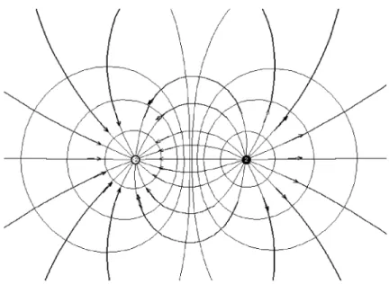
FIGURE 15.4 Electric dipole field map with equipotentials. Note in this case the equipotential surfaces are not spheres, but are everywhere perpendicular to the electric field. Make sure you are clear on the difference between electric field lines and equipotentials. Which are which in the figure?

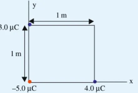
EL E C T R I C DI P O L E S A N D CH A R G E DI S T R I B U T I O N S 3 7 9 1 m 1 m 3.0 μC –5.0 μC 4.0 μC x y

Example 15.2Calculate the potential and the electric field at the empty corner

of a square of 1 m sides when there are point charges at each of the other cor-ners as shown.

One particular arrangement of two charges that is of general significance is the

elec-tric dipole already studied in Examples 14.2 and 14.3. Its significance lies in the fact that

even though it is electrically neutral, the separation of positive and negative charges allows it to produce an electric field and corresponding electric potential.

Electric dipoles of two types occur in nature. A net separation of equal positive and negative charges may be permanent, as, for example in the important case of the water molecule (Figure 15.7). Even molecules that are electrically neu-tral and have no permanent dipole moment can, in the presence of an external electric field, form a dipole moment by a process known as electric polariza-tion. The imposed electric field causes a separation of positive and negative charges in the otherwise neutral molecule leading to an induced dipole moment. This important process is discussed in more detail in the next section.

To calculate the electric potential of a dipole, we first specify a coordinate system and then use Equation (15.9) to add the individual

observation point

qi

ri

FIGURE 15.6Geometry to calculate potential from a distribution of point charges.

Solution: We first calculate the electric potential at the empty corner of the

square. Because potential is a scalar, we simply add the potential due to each charge, as in Equation (15.9), to find

The factor is the length of the diagonal of the square, the distance from the ⫺5␮C charge to the observation point. To find the electric field at the same point we must add the electric field vectors produced by each point charge at the observation point. This sum is given, in ordered pair notation, by

where the direction of the field from the ⫺5␮C charge is along the diagonal of the square toward the charge and we have taken its x- and y-components. Combining terms, the net electric field is

In general, it is clearly easier to calculate scalar electric potentials than vector electric fields. E : ⫽11.1⫻104_{, 2.0⫻10}421_V/m2_. a⫺5⫻10⫺6 (12_⫹12 ₎ cos 45, ⫺5⫻10⫺6 (12_⫹12 ₎ sin 45b d, E: ⫽ 1 4pe_°c a 3⫻10⫺6 12 ,0b⫹ a0, 4⫻10⫺6 12 b⫹ 32 V⫽ 1 4pe_oc 3⫻10⫺6 1 ⫹ 4⫻10⫺6 1 ⫺ 5⫻10⫺6

1

potentials. If we choose the arrangement shown in Figure 15.8, we find the poten-tial to be

(15.10)

where r_⫹and r_⫺are the respective distances of the positive and negative charges to the observation point. If the observation point is much farther away than the size of the dipole d, so that with r⫽r_⫺~ r_⫹⫹ ⌬r as shown in Figure 15.8, then from the figure,

we can write that

where ␪is the angle between the vector from the dipole center to the observation point and the dipole axis, chosen by a convention in which the axis points from neg-ative to positive charge along the dipole. Substituting this into Equation (15.10) results in

(15.11)

where we have defined the electric dipole moment to be p⫽qd, equal to the

magni-tude of either charge times the charge separation distance.

The electric potential of a dipole differs from that of an isolated charge in two sig-nificant ways. First, the dipole potential decreases much faster with increasing distance, varying as 1/r2 _{whereas the potential of a point charge varies as 1/r. This is to be} expected because the net charge of the dipole is zero and the force on, or the interac-tion energy with, a charge at the observainterac-tion point is expected to be substantially less than that due to a single charge q at the site of the dipole (see the example just below). Second, the dipole potential is no longer spherically symmetric, but has an angular dependence. This is also to be expected because the dipole has a symmetry axis defin-ing a preferred direction in space.

V⫽qd cosu 4pe_o r2⫽ p cosu 4pe_o r2, r : c_r1 ⫹⫺ 1 r_⫺d ⫽ r_⫺⫺r_⫹ r_⫹ r_⫺ ⫽ ¢r r2 ⫽ d cos u r2 , V_dipole⫽ 1 4pe_oc q r_⫹⫺ q r_⫺d, Observation point +q –q d r+ r– r Δr θ

FIGURE 15.8Geometry for electric dipole calculation.

+

_

+

FIGURE 15.7 Molecular struc-ture of the water molecule. The red oxygen carries a partial negative charge, and the blue hydrogens each carry a partial positive charge so that there is a separation of the centers of positive and negative charge producing a permanent dipole moment for water.

EL E C T R I C DI P O L E S A N D CH A R G E DI S T R I B U T I O N S 3 8 1

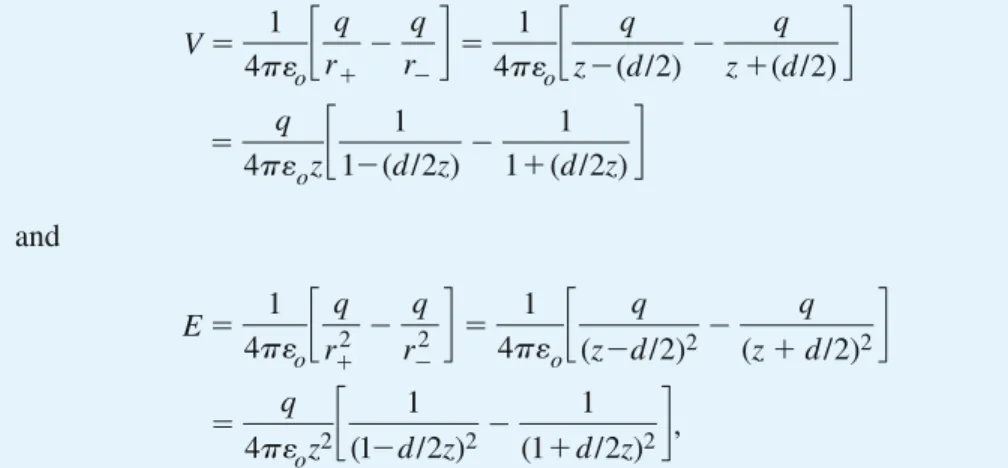
Example 15.3 Calculate the electric potential and field of an electric dipole

along its axis.

Solution:Using the notation of Figure 15.8 as applied to an observation point

along the dipole axis, say the z-axis, we can write expressions for the electric potential and field of a dipole as

and

where points along the z-axis. To proceed, we simplify the final term in the bracket of each expression using the binomial theorem when

to find

and

We compare the z-dependence of these two expressions, per unit dipole moment, in Figure 15.9. Note the faster decrease in E with distance from the dipole, varying as 1/z3_{versus the 1/z}2_{variation of V.}

E⫽ q 4pe_o z2

C

D

C

D

FIGURE 15.9Electric potential (1/r2_{, lower dashed line) and field (1/r}3_{, solid line in}

blue) along the axis of a (unit) electric dipole. The plots have been normalized to

coincide at the maximum value shown. Upper curve (red) has a 1/r dependence, for comparison.

Continuous distributions of electric charge, in which the charge is found throughout a volume or on a surface, are obviously more common real-life examples of actual charge distributions than point charges. Most of these sit-uations must be handled using numerical methods on a computer, but if there is sufficient symmetry in the geometry of an object on which the charge resides then analytical expressions for the potential can be obtained using calculus. One useful representation for the electric potential of a charge dis-tribution is a potential map, very much like a topological map. An example is given in Figure 15.10 for a protein molecule. Such mappings are particu-larly useful for visualizing the potential in the neighborhood of a complex macromolecular surface that would be detected by a small ion or molecule.

4. ATOMIC AND MOLECULAR ELECTRICAL

INTERACTIONS

Our current understanding of the electrical interactions between elementary constituents of matter comes from quantum mechanics, a subject we explore briefly toward the end of this book. One ultimate question in our fundamental understanding is why atoms are sta-ble objects. Consisting of a positive nucleus and negative electrons that, according to Coulomb’s law, should attract each other, they might be expected to be unstable and col-lapse. The negative potential energy curve of Figure 15.1 corresponds to this situation. An electron would be expected to “fall” down this potential energy hill to the nucleus at the origin. We show later how quantum mechanics addresses this fundamental question but for now we simply treat atoms as stable objects. As two atoms approach each other, once their electron clouds (for now, a vague term that indicates the rough size of an atom) over-lap, there is a very strong repulsive force arising from quantum mechanical effects. This very strong repulsion is sometimes called a hard-sphere repulsion because it resembles the strong repulsive interaction between two billiard balls that prevents them from overlap-ping in space when they come into contact. As long as atoms do not overlap in space, we will have a reasonable degree of understanding of their electrical interactions by treating them as point charges and dipoles and ignoring quantum mechanics.

Atomic distances are usually measured in angstroms (Å), where 1 Å⫽0.1 nm. The smallest atom, hydrogen, has a diameter of about 1 Å, whereas the largest atoms are only several Å in diameter. If we calculate the magnitude of the electric potential energy due to the Coulomb interaction between two electrons, separated by a distance of 1 Å, we find from Equation (15.2),

(For comparison with bond strengths discussed in Section 5 of Chapter 12, this energy corresponds to

about 4–5 times larger than the energy of the strongest atomic bonds that exist.)

We can classify the various types of electrical interactions possible between atoms or molecules. The strongest interactions are those due to direct charge–charge interactions, having a potential energy given by Equation (15.2), but with the permittivity of vacuum ␧_o modified by the electrical properties of the medium in which the charges are immersed (discussed in the next section). With one charge at the origin, the potential energy of such interactions decreases with separation distance as 1/r. Charge–charge interactions only occur between two

PE⫽2.3⫻10 ⫺19 _J/bond

#

FIGURE 15.10The acetylcholine esterase molecule with two types of color coding. On the left, the surface is color-coded with positive

(blue) and negative (red) charges

(with the dipole moment shown as the white arrow), whereas on the right two equipotential surfaces are mapped, each corresponding to k_BT energy (GRASP modeling).

It is interesting to check that we can calcu-late the electric field for Example 15.3 directly from the expression for the electric potential using Equation (15.7). To find E_z we simply differentiate V with respect to z:

in agreement with the separate and more difficult calculation in the example.

⫽ ⫺1⫺22p 4pe_o z3⫽ p 2pe_o z3, E_z⫽⫺dV dz ⫽ ⫺ ⫺ d dzc p 4pe_o z2d

ionized atoms or molecules, both having net charge. Other types of electrical interac-tions are discussed in decreasing order of strength based on their dependence on sep-aration distance.

The charge–dipole interaction occurs when one atom or molecule is charged and the other has a permanent dipole moment. According to Equation (15.4), the interaction potential energy should be given by the product of the charge and the dipole potential, given by Equation (15.11). In this case the potential energy decreases with separation distance as 1/r2_{and is proportional to the product} of the charge and dipole strength, also depending on the orientation of the dipole in space.

If both atoms or molecules have no net charge but are permanent dipoles then the

dipole–dipole interaction occurs with an energy that varies as 1/r3_{and depends on} the two dipole strengths as well as their relative orientation in space. All of the above interactions can be either attractive or repulsive, resulting in potential energies that are either negative or positive, respectively.

When one of the atoms or molecules has both no net charge and no permanent dipole moment, it can still interact electrically with a charge on another atom or mol-ecule. The charge creates an electric polarization (or separation of positive and neg-ative centers of charge) of the neutral atom or molecule so that an induced dipole is formed (Figure 15.11). The charge–induced dipole interaction is always attractive because the induced dipole is always created with the opposite charge closest to the original isolated charge. The interaction dies away faster still with separation dis-tance, varying as 1/r4_.

What is the situation when both atoms (or molecules) have neither a net charge nor a permanent dipole moment? Will they still interact electrically? All atoms are composed of a number of electrons and an equal number of protons in the nucleus. The time average of the electric dipole moment will be zero, because we have assumed no permanent dipole. However, over short time intervals there will be a nonzero rapidly varying dipole moment that can interact with a second neighboring neutral, nonpolar atom or molecule to induce a corresponding electric polarization and induced dipole moment. Known as the dispersion interaction, this interaction is always attractive, just as for the case for the charge-induced dipole interaction. Varying as 1/r6_{it is the most rapidly decaying attractive force} between atoms or molecules and is only significant for two molecules that are in very close proximity.

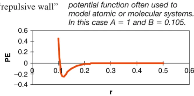
The total potential energy function for the interactions between two atoms or molecules is the sum of all the interaction energies. It will, of course, depend on the details of the particular atoms or molecules, but for many purposes can be accurately modeled by combining a positive (repulsive) hard-sphere potential energy function with a negative (attractive) longer-range potential energy function. One commonly used form for neutral nonpolar atoms or molecules is the Lennard–Jones or “6–12” potential function

(15.12)

a plot of which is shown in Figure 15.12. This function displays most of the usual features seen in atomic or molecular systems. There is a very steep “repulsive wall” at the closest approach distances representing the hard-sphere

repulsion. The minimum represents the equilibrium separation distance (at 21/6_{B) for the two particles. Beyond the minimum,} the slope becomes positive indicating an attractive force (recall Equation (15.8)) and there is a much less steep “attractive tail” that reaches a nearly neutral plateau beyond about 2B. With the parameters A and B chosen for the particular system, this poten-tial form is a generally useful approximation.

PE(r) ⫽ 4Ae aB rb 12 - a B rb 6 f, AT O M I C A N D MO L E C U L A R EL E C T R I C A L IN T E R A C T I O N S 3 8 3 ++++++++ + – – – – + + + p +

FIGURE 15.11A charged rod inducing a net dipole on a neutral sphere. –0.4 –0.2 0 0.2 0.4 0.6 0 0.1 0.2 0.3 0.4 0.5 0.6 r PE

FIGURE 15.12The Lennard–Jones potential function often used to model atomic or molecular systems. In this case A⫽1 and B⫽0.105.

5. STATIC ELECTRICAL PROPERTIES

OF BULK MATTER

Having described the fundamental nature of conductors and insulators, let’s examine and contrast some of their properties in the presence of an electric field. As we have seen in Section 4 of the previous chapter, at electrostatic equilibrium any excess charge on a conductor resides on its surface and the electric field inside a conductor is zero even when the conductor is placed in an external electric field. Furthermore, at equilibrium the electric field at the external surface of the conductor is always perpendicular to its surface. In the language of electric poten-tial, the surface of a conductor is an equipotential (Figure 15.13). No work is required to move charges on the conductor’s surface or throughout its interior as well, since all portions of the conductor are at the same potential.

In the case of an insulator in an electric field, charges are not free to migrate in response to the field. We can distinguish two types of insulators based on whether the molecules have a permanent dipole moment. In polar dielectrics, those with a per-manent dipole moment, the dipoles will tend to align in the external electric field to some extent. This alignment is due to a torque on the dipole p from the interaction with the electric field E. In a uniform electric field each of the dipole charges q will experience the same force qE, resulting in equal but opposite forces on the dipole (known as a couple). The resulting torque on each charge about the dipole center is equal to (see Figure 15.14) so that the net torque is given by

(15.13) where d is the dipole length and ␪is the angle between the dipole and the electric field. This torque will tend to align the dipole with its axis along the E field direction. However, they will not all completely align with the field because of thermal motions that tend to randomly orient the dipoles. Only if the external electric field is quite large and/or the temperature is sufficiently low will the dipole alignment be essen-tially complete.

A dipole in an electric field will have a potential energy corresponding to the work done by the torque in rotating the dipole. In a uniform electric field this poten-tial energy can be shown to be

(15.14) where ␪ is defined just as in Equation (15.13) to be the angle between p and E As expected, the lowest energy (PE_p⫽ ⫺pE) occurs when the dipole is oriented

along the E field, a position of stable equilibrium, and the highest energy occurs when p and E point in opposite directions (PE_p⫽pE), a position of unstable

equi-librium. When the dipole is oriented along the E field small perturbations in its orientation lead to a restoring torque as seen in Figure 15.14, but when the dipole is aligned oppositely to the field a small perturbation will lead to a large torque that tends to flip its orientation to line up with These energy ideas are important in later discussions.

When nonpolar dielectrics are placed in an external electric field, the molecules become polarized, with their electrons shifting the center of charge away from that of the nuclei in the direction of E, producing an induced dipole moment (Figure 15.15). The extent of this polarization, and therefore the magnitude of the induced dipole moment, depends on the electrical characteristics of the particular molecules.

In any case, when a slab of dielectric, either polar or nonpolar, is placed in an electric field, the net result is to create surface charge layers on the slab as shown in Figure 15.16. There is no net charge throughout

E:. B B B B B PE_p⫽ ⫺pE cos u,

t⫽qEd sinu⫽pE sinu,

Fr_⬜⫽qE(d /2)sin u, F=qE E F=qE –q _d +q p _θ

FIGURE 15.14A couple is exerted on a permanent dipole in a uniform E field.

FIGURE 15.13Electric field and equipotential surface for a conductor. The electric field is greatest where the curvature is greatest; equipotential surfaces are bunched where the field is largest. The metal surface itself is an equipotential.

the dielectric volume, but because of either the orientation of polar dielectric mol-ecules or the induced dipole of nonpolar dielectrics, surface layers of charge are present. The net effect of these surface charges is to reduce the electric field within the dielectric through a partial shielding. Unlike in a conductor, where the free charges can move in response to an electric field and distribute themselves on the surface so as to cancel the electric field within the conductor, dipoles in a dielec-tric can only partially reduce the internal elecdielec-tric field. The extent of field reduc-tion depends on the dielectric material and is characterized by the dielectric

constant␬, a dimensionless number that indicates the factor by which the internal electric field is reduced compared to its value in vacuum

(15.15) Table 15.1 lists some values for dielectric constants of various insulating materi-als. Note the extremely high dielectric constant of water indicating that water is a very good insulator. This seems contrary to common knowledge that, for example, it is dangerous to be in water during an electrical storm. The conductivity of water is due entirely to the ionic content of the water. Pure water itself is a very poor con-ductor of electricity.

E⫽Eo

k.

STAT I C EL E C T R I C A L PR O P E R T I E S O F BU L K MAT T E R 3 8 5

p

FIGURE 15.15(left) Nonpolar atom with centers of positive (blue) and

negative (red) charge overlapping; (right) same atom in a uniform electric field, with center of negative charge shifted to the left creating an electric dipole along the electric field.

_ _ _ _ _ _ _ + + + + + + + Eexternal Eexternal Enet internal Einduced Eexternal

FIGURE 15.16The net internal E field is the superposition of the external field (light green) and the internal field due to the induced surface charges (red). It is always reduced due to the shielding of the induced charges.

Table 15.1Dielectric Constants of Some Insulating Materials

Material Dielectric Constant

Air 1.00054 Paper ~4 Pyrex glass 4.7 Rubber (Neoprene) ~7 Ethanol 25 Water 80

Recently scientists have developed methods to calculate accurate electric poten-tials near the surface of a macromolecule. This has been a significant advance in our understanding of the interplay of native structure and function and also in our ability to design synthetic new macromolecules not found in nature. Macromolecules are inherently highly charged structures immersed in an ionic environment, whether inside a cell or in a buffered solvent in a test tube. The charges on macromolecules, such as proteins or nucleic acids, play a major role in determining the native structure of the molecule as well as its functioning. Specific small molecules that bind to a macromolecule, known as ligands, may be recognized not only by their size and

shape, but also through their charge interactions. Charge groups near an active site on an enzyme may play a role in regulating the bind-ing rates of ligands.

These electric potential calculations require a detailed knowl-edge of the three-dimensional structure of a macromolecule, com-plete with the locations of all its atoms. A catalog of the comcom-plete structure of many proteins is rapidly growing and is available in computer databases. In one widely used calculational scheme, a cubic lattice grid of points (like three-dimensional graph paper) is chosen and values for charge density, dielectric constant, and ionic strength parameters are assigned to each lattice point. The surface of the macromolecule is usually taken as the so-called van der Waals (or hard-sphere) envelope of the surface atoms and a low internal dielectric constant (2 – 4) is chosen to represent a mean value whereas a large value (~80) is assigned to external lattice sites to represent the aqueous solvent. At this point the problem becomes a classical electrostatics calculation with a large set of point charges given at known locations. The qualitative presentation in Section 3 above is used in a more quantitative form to write down the mathematical problem and numerical methods have been developed in order to calculate the electric poten-tial. Those methods have been greatly improved in recent years so that fairly rapid calculations can now be performed and these improvements have led to a rebirth in the application of electrostatics to the study of macromolecular interactions.

The three-dimensional mapping of the electric potential (see color-coded examples in Figures 15.10 and 15.17) reveals patterns of interaction energies that are not at all apparent from the three-dimensional structure of the macromolecule itself. Patterns of positive or negative potential can be seen over the surfaces of macromolecules and such specific potential features near an active site for binding of a ligand can give important information on the electrostatic interactions with the ligand. Studies of similar macro-molecules can show the importance of various specific portions of those structures.

A general knowledge has been assembled on the electrostatic effects of various common structural elements found in proteins and nucleic acids and this body of knowledge has been extremely useful in de novo protein design, the planning and fabrication of new proteins not known to occur in nature. Since the mid 1980s sev-eral such proteins have been designed and made. So far they have not been designed with the idea of inventing important new macromolecules, but rather to test fundamental notions on the relationship between structure and functioning of macromolecules by designing simplified macromolecular “motifs”. For example, a number of proteins have been created to act as membrane channels (see below) in order to test ideas on the minimum necessary characteristics of such proteins to allow a functioning channel. Knowledge gained in these endeavors will no doubt lead to the future development of new proteins able to perform specific biological functions in living tissue, perhaps replacing the function of defective proteins.

6. CAPACITORS AND MEMBRANES

The lipid bilayers of cell membranes can be electrically modeled as a sandwich consisting of two layers of a conductor (the plane of the polar lipid heads) sepa-rated by a dielectric layer (the hydrocarbon tails; see Figure 15.18). Such an elec-trical arrangement is known as a capacitor, or sometimes a condenser. When made of metals and insulators this is a common device for storing electric potential energy and is found in essentially all electronic devices, from telephones to com-puters. Surrounding a cell, the lipid bilayer provides a barrier to maintain a differ-ent internal environmdiffer-ent of ions and macromolecules from the extracellular bathing fluid. Because of an unequal distribution of various ions between the inside and outside of all living cells, there is an electric potential difference across

FIGURE 15.17Two color-coded images of the protein lysozyme. The left image is coded by curvature and shows a major bind-ing cleft for polysaccharides, whereas the right image is coded by electrostatic charge and shows a highly negative (red ) binding site in an otherwise positively charged

(blue) lysozyme. Computer

model-ing has allowed these detailed pictures only in recent years.

all cell membranes known as the resting potential. Its magnitude varies according to cell type, but the inside of cells is always negative with respect to the outside and the magnitude of the potential difference is roughly 100 mV or 0.1 V and is rela-tively constant.

Certain types of cells have evolved to respond to particular types of stimuli (elec-trical, chemical, or mechanical) all with the same basic signal, a transient change in the membrane potential (depolarization of the membrane), followed by a restoration of the resting potential (repolarization). Such cells include nerve, muscle, and sensory cells, all having a similar basic membrane structure. We first develop some concepts about the storage of charge on a generic capacitor before returning to consider the capacitance and charge properties of membranes.

As we have seen, the work done in assembling any array of electric charges results in an electric potential energy. A device used to store electric charge will also thereby store energy. Any array of conductors will serve this function and act as a capacitor, but several simple geometries using two conductors (known as the plates of the capac-itor) usually separated by a dielectric are most often used. Figure 15.19 shows some examples of common capacitors used as electrical devices.

Consider a parallel-plate capacitor shown in Figure 15.20. Such a capac-itor is a prototype for all capaccapac-itors and even the electrical symbol for a capacitor resembles a parallel-plate capacitor. If made with thin metal foil conductors and dielectric layers in between, the plane sheets can be rolled up to form a compact cylindrical device. In introducing capacitance, we first assume that there is no dielectric layer between the plates but just vacuum. Suppose equal and opposite charges ⫾Q are placed on the two plates. There

will then be an electric field between the two plates and a corresponding potential difference that we denote by V. In general, the charge Q on either plate of a capacitor and the potential difference across the plates are propor-tional, defining the capacitance C by

(15.16) From the boxed calculation in Section 4 of Chapter 14, the electric field from a plane sheet of charge is E⫽␴/2 , where ␴ is the charge per unit area (Q/A) on the sheet. For the parallel plate situation of Figure 15.20, the fields produced by each plate add in the space between the plates, but

e_o

Q⫽CV.

冷

冷

CA PA C I T O R S A N D ME M B R A N E S 3 8 7

FIGURE 15.19Variously packaged common capacitors.

FIGURE 15.18Two models of a lipid bilayer with polar heads on the surface and hydrocarbon tails buried within. The image on the right also shows an ␣-helical transmembrane polypeptide.

where Q and A are the charge on an area of one of the plates. Because E is a constant, the potential difference between the plates is given by Equation (15.6) as

(15.18)

where d is the plate separation. From Equations (15.16) and (15.18), we find that the capacitance of the parallel-plate capacitor is given by purely geometric factors as

(15.19)

The fact that the capacitance depends entirely on geometry is a general result, regardless of the capacitor’s shape. Units for capacitance are given by those of Q/V or 1 C/V⫽1 farad (F). A farad is an enormous value for capacitance and units of pF to ␮F are common.

A charged capacitor not only stores charge, but also energy. For a parallel-plate capacitor we can calculate the stored energy from the following argument. Imagine the plates to be initially uncharged and the charging to occur by the transfer of elec-trons from one plate to the other in a process that results in equal but opposite final charges. After the plates have been partially charged and the potential is at some intermediate value V⬘between 0 and the final potential V, in order to transfer a small additional amount of charge ⌬q we need to do an amount of work equal to ⌬q V⬘. To transfer a total amount of charge Q, we cannot simply multiply the final charge and potential together because the potential changes in proportion to the amount of charge transferred. However, we can obtain the correct value for the work done by imagining that instead of continuously transferring charge, we transfer all of the charge Q through a constant potential difference that is equal to the average value during the actual process. Because the average potential is V/2 (see Figure 15.21), we find that the work done is W⫽Q(V/2) The potential energy stored in the

capac-itor is then equal to

(15.20)

Because in the actual charging process both Q and V vary with time, it is often useful to rewrite Equation (15.20) in terms of the capacitance and only one vari-able, using Equation (15.16). Substituting for either Q or V in Equation (15.20), we obtain three equivalent forms for the stored energy of a capacitor,

PE⫽1 2 QV. C⫽eo A d . (parallel⫺plate C). V⫽Ed⫽ Qd e_o A,

FIGURE 15.20A charged parallel plate capacitor, showing the cancellation of electric fields outside and net E field within the capacitor. The electric field from each plate is constant and points either away from the positive or toward the negative plate. Superposition of these electric fields leads to confine-ment of the electric field between the capacitor plates.

V

Charge on capacitor Q

Potential across capacitor

V=V / 2

FIGURE 15.21The potential across the capacitor increases linearly with the charge on the plates. The same work (equal to the area under the diagonal line) is done in charging the plates continuously as would be done by transferring charge Q across the average potential of V/2 (area under the heavy dashed line).

+Q _–Q E+ E+ E+ E– E– E– Enet=0 Enet=0 Enet

cancel in the space outside the plates as shown. The electric field between the plates (away from the edges where boundary effects occur) is therefore constant and given by

(15.17)

E⫽ Q

e_o A,

(15.21)

An example may help to clarify the appropriate use of these expressions. PE⫽1 2 QV⫽ 1 2CV 2_⫽1 2 Q2 C.

CA PA C I T O R S A N D ME M B R A N E S 3 8 9

Example 15.4This is our first example of an electrical circuit. We want to find the

charge on the 10⫻10 cm plates of a parallel-plate capacitor (shown below on the right) with a 1 mm air gap after it is connected to the terminals of a 12 V battery as shown.

Solution:The figure shows both the actual physical arrangement and the

elec-trical circuit diagram used to represent the situation. Note that the symbol for a battery (with “⫹⫹”, longer line, and “⫺⫺”, shorter line, terminals) is somewhat similar to that for a capacitor (with equal length lines) and that the drawing of connecting wires is arbitrary as long as they have the same connections at their ends. The battery is a device that supplies a potential difference, or voltage, between its two terminals. When the switch shown in the diagram is closed, charge flows from the battery onto the capacitor plates until the voltage across the capacitor plates reaches the same value of 12 V that is across the battery ter-minals. At this point the two separate “halves” of the circuit, the left and right portions of the circuit diagram corresponding to the two physically separated metal parts of the circuit, divided by the air gap in the capacitor and the battery acid within the battery, are each equipotential surfaces and no further charge flows. The positive side of the circuit is at a potential of 12 V with respect to the 0 V of the negative side.

To determine how much charge flows, we must first calculate the capaci-tance of the parallel-plate capacitor using Equation (15.19). We find

The amount of charge on each plate of the capacitor is then found from the def-inition of capacitance, Equation (15.16), to be

with the plate attached to the positive battery terminal with⫹1.1 nC and the other plate with ⫺1.1 nC of electric charge.

Q⫽CV⫽88⫻10⫺12 _{F⫻12 V⫽1.1⫻10}⫺9 _C,

C⫽eo A d ⫽

8.85⫻10⫺12 _(0.1⫻0.1)

0.001 ⫽88 pF.

What does it mean that the work done in charging a capacitor is stored as poten-tial energy? One view is that the energy is stored in the configuration of charges and that if the two capacitor plates are connected by a conductor, electrons on the nega-tive plate will gain kinetic energy and rapidly flow to the other, posinega-tive, plate, thus neutralizing both plates. We discuss this further in the next chapter where we discuss the flow of electric charge.

Another equivalent, but perhaps more revealing, view is that the energy is stored in the electric field that is created between the capacitor plates. If we substitute for C and V from Equations (15.18) and (15.19), we can find an expression for the potential energy that depends only on E and the geometry of the plates

(15.22) The product Ad is just the volume between the capacitor plates that the electric field fills uniformly without extending outside the capacitor, thus Equation (15.22) states that there is an energy per unit volume, or energy density, stored in the electric field and given by

(15.23) This is a fundamental relationship for the energy stored in an electric field. Despite the rather specialized example used to derive this result, we show later that it is indeed a very general and important result that is not restricted to capaci-tors. The fact that there is energy in the electric field, and that the energy is proportional to the square of the field, leads us to many significant developments in electromagnetism.

If a dielectric material with dielectric constant ␬fills the space between the plates, then, as we have seen, the internal electric field is reduced by the factor ␬. With a given charge Q on the plates, the presence of the dielectric reduces the potential difference between the plates by the same factor ␬(because according to Equation (15.6) V

μ

so that the capacitance is thereby increased by the factor ␬ (because according to Equation (15.16) C

μ

(15.24) where the initial values are those without the dielectric.

With a good insulator, capacitance values can be substantially increased. The increase in capacitance with a dielectric implies (from Equation (15.22)) that if the volt-age across the capacitor is maintained constant by a battery, for example, then the stored energy and charge will both increase by a factor ␬relative to the same capacitor without a dielectric. On the other hand, Equation (15.23) implies that because the elec-tric field decreases by ␬, E2_{should decrease by a factor of ␬}2_{, whereas the term ␧}

␱is

multiplied by a factor of ␬, so that the energy stored should decrease by a factor of ␬ relative to the same capacitor without a dielectric. The following example should help to clarify this apparent paradox.

V⫽Vo k; C⫽Cok, PE (Vol.)⫽ 1 2eo E 2_. PE⫽1 2CV 2_⫽1 2 a e_o A d b(Ed) 2_⫽1 2 eo E 2 _Ad.

Example 15.5A 0.1␮F parallel-plate capacitor is charged by a 12 V battery and

dis-connected from the battery. A slab of dielectric with ␬⫽4 is then inserted to fill the gap in the capacitor. Find the charge on the capacitor plates and the voltage across the plates before and after inserting the dielectric. If the capacitor is then reconnected to the battery, how much more, if any, charge will flow onto the capacitor?

Solution:When connected to the battery, the capacitor will be

charged to 12 V and will have Q⫽CV⫽(0.1␮F)(12 V)⫽ 1.2␮C of charge on each plate. After the capacitor is discon-nected from the battery, this charge will remain on the capac-itor. (We show in the next chapter that for a real (nonideal) capacitor, the charge will, in fact, slowly leak off, but we

+ + + + – – – – – – – – – – + + + + + +

So, the resolution of the apparent paradox presented before this example is that the resulting energy stored depends on whether the capacitor has its voltage fixed, while attached to the battery, or has its charge fixed, when isolated. In the first case additional charge will flow onto the capacitor to maintain the voltage fixed at the battery value, whereas in the second case the field and voltage will decrease because of the dielectric screening.

The capacitance per unit area (specific capacitance) of cellular membranes was first determined in the 1920s to have a value of about 1␮F/cm2_{. This number was} used to estimate the thickness of the previously undetected cell membrane using the parallel-plate relation for capacitance (Equation (15.19) multiplied by the factor ␬)

C/A⫽␬␧_␱/d. Using a value of ␬⫽3 (based on the knowledge that membranes con-tained lipids and that oils have a value of ␬~ 3) and the measured value for C/A, an estimate for the membrane thickness of d ~ 3 nm was obtained (you can verify this). Although today we know that most membranes are about 7.5 nm thick, this was the first such determination and indicated that the membrane thickness might corre-spond to the length of a macromolecule.

Assuming that the charge on a cell membrane is uniformly distributed, we can obtain an estimate of how much charge lies on a membrane. From Equation (15.15), by dividing both sides by the area of the membrane, we obtain

(15.25) If we take V⫽0.1 V and a capacitance per unit area of 1␮F/cm2, then we find a charge per unit area of 0.1␮C/cm2. We can get a feeling for this charge density on the membrane by calculating the average spacing of the individual charges on the membrane surface. With x equal to the average separation between charges on the membrane surface, so that there is one charge per surface area x2(see Figure 15.22), we can find a value for x from

so that, solving for x, we find that there is one charge every x⫽13 nm in a square array over the surface of the membrane.

1 charge x2 _cm2 ⫽ 0.1⫻10⫺6 _C/cm2 1.6⫻10⫺19 _C ⫽6.25⫻1011 charges/cm2 , Q A⫽ C AV. CA PA C I T O R S A N D ME M B R A N E S 3 9 1

ignore that here.) When the dielectric is inserted, the charge still remains on the capacitor, but the dielectric will have an induced layer of surface charge that will shield the charge on the metal plates (see the figure) and reduce the electric field and the potential within the capacitor by a factor of (1/␬). Accordingly, the poten-tial is reduced to V⬘ ⫽12/4⫽3 V.

Equation (15.23) tells us there is a corresponding decrease in potential energy stored in the capacitor by a factor of (1/␬). What happened to this energy? As the dielectric is inserted between the capacitor plates, the induced charges on the dielectric cause an attractive force pulling the slab into the gap between the capacitor plates. In terms of overall energy conservation, negative work has to be done on the dielectric by an external agent, using an external force to hold the slab back from accelerating into the gap, in order to position the dielectric within the capacitor. A careful calculation shows that this negative work just balances the decrease in stored potential energy.

If the capacitor is then reconnected to the battery, the potential across the plates will again rise to 12 V with the transfer of additional charge to the metal plates. The total charge on the plates is then given by the product of the voltage and the capacitance (now increased by a factor of ␬), Q_total⫽(12 V)(0.4␮F) ⫽4.8␮C, so that an additional (4.8⫺1.2)⫽3.6␮C of charge was transferred to the plates.

We can also calculate the electric field inside the membrane from Equation (15.18). Substituting V⫽0.1 V and d⫽3 nm, together with a reduction in E by the factor ␬⫽3, we find that E⫽1.1⫻105_{V/cm, an extremely high value. In fact, the} largest possible E field in dry air is only 0.3⫻105_{V/cm, with higher E fields in air} causing dielectric breakdown. Such large E fields in membranes are responsible for relatively large forces on molecules within membranes, suggesting that by proper triggering, much energy can be released through interaction with the electric field.

Although the membrane capacitance can be approximated by an expression for a parallel-plate capacitor, it should be pointed out that the electrical properties of a membrane are quite a bit more complex than an ideal capacitor. As we show in the next section and again in the next chapter, membranes do allow a flow of charge through specific pores known as channels. Furthermore, along membranes in large cells such as nerve or muscle, the properties of the membrane vary both spatially along the membrane and with time. Membranes are indeed far from passive con-ducting plates separated by an ideal insulator. They are dynamic structures with very complex electrical properties capable of rapidly changing the ionic environment of a cell, of transporting large macromolecules across the cell barrier, and of propagat-ing electrical signals rapidly over long distances.

7. MEMBRANE CHANNELS: PART 1

Membrane channels are specific integral membrane protein/sugar/fatty acid

com-plexes that act as pores designed to transport ions, water, or even macromolecules across a biological membrane (see Figure 15.23). Channels play a distinctive role in excitable cells, such as neurons and muscle cells, where they control the flow of ions and the subsequent generation of electrical signals. In this section, we learn some fun-damentals of the general nature of channel structure and functioning in anticipation of a fuller discussion of the role of channels in nerve conduction in the next chapter.

There are probably hundreds of different specific channels in various types of mam-malian cells. Although first studied and modeled by Hodgkin and Huxley in the early 1950s in ground-breaking experiments, channels have recently been studied using a large array of techniques including modern electrophysiology, biochemistry, and molecular biology. In a simple picture, channels can be said to exist in either of two states, open or closed, in which specific ions or small molecules can either pass through the channel “gate” or not. Control of the gating of a channel can be either by specific charges

(volt-age-gating) or by the binding of small molecules (ligand-gating). Ligand-gated channels

include those for neurotransmitters and small proteins involved in other forms of cell signaling. Voltage-gated channels are present in nerve and muscle and we focus on these in our discussion.

To give a more concrete idea of what a channel is and how it functions in a cell membrane, let’s consider the sodium ion channel in some detail. The Na channel is formed by a complex of a single polypeptide chain of about 2000 amino acids with associated sugars and fatty acids. This single chain has four similar subunits, each composed of six helical portions, with each of these spanning the membrane so that the overall struc-ture resembles that shown in Figure 15.24. The Na channel has been purified and shown to be functionally active when recon-stituted in pure lipid membranes. In muscle, there are between 50 and 500 Na channels per ␮m2 on the membrane surface. Each of these is normally closed, but can be opened by a change in the electric potential across the membrane. The open state is short-lived, lasting about 1 ms, during which time about 103Na⫹ions flow into the cell through each channel from the higher Na⫹ion-rich extracellular medium. When the channel is open, the flow is highly selective for Na⫹ions, with potassium (K⫹) ions some 11 times less likely to cross the Na channel.

FIGURE 15.23Molecular model of a membrane showing a channel in the form of a mostly helical protein that spans the membrane (shown in blue) allowing selected ions to enter or leave the cell.

FIGURE 15.22A uniform surface charge model for a cell

membrane with one charge centered in each box.