arXiv:astro-ph/0501591v1 26 Jan 2005
Gary Steigman
The Ohio State University, Columbus OH 43210, USA
Abstract. The relic abundances of the light elements synthesized during the first few minutes of the evolution of the Universe provide unique probes of cosmology and the building blocks for stellar and galactic chemical evolution, while also enabling constraints on the baryon (nucleon) density and on models of particle physics beyond the standard model. Recent WMAP analyses of the CBR temperature fluctuation spectrum, combined with other, relevant, observational data, has yielded very tight constraints on the baryon density, permitting a detailed, quantitative confrontation of the predictions of Big Bang Nucleosynthesis with the post-BBN abundances inferred from observational data. The current status of this comparison is presented, with an emphasis on the challenges to astronomy, astrophysics, particle physics, and cosmology it identifies.
1
Introduction and Overview
Our Universe is observed to be expanding and filled with radiation (the Cosmic Background Radiation: CBR), along with “ordinary” matter (baryons≡ nucle-ons). It is well known that if this evolution is followed backwards in time, then there was an epoch during its early evolution when the Universe was a “Primor-dial Nuclear Reactor”, synthesizing in astrophysically interesting abundances the light nuclides D,3He,4He, and 7Li. Discussion of BBN can start when the Universe was some tens of milliseconds old and the temperature (thermal en-ergies) was of order a few MeV. At that time there were no complex nuclei, only neutrons and protons. Since there are nearly ten orders of magnitude more CBR photons in the Universe than nucleons, photodissociation ensures that at such high temperatures the abundances of complex nuclei are negligibly small. However, as the Universe expands (and the weak interactions transmute neu-trons and protons), collisions among nucleons begin to build the light nuclides when the temperature drops below∼100 MeV, and the Universe is a couple of minutes old. Very quickly, almost all neutrons available are incorporated in the most tightly bound of the light nuclides, 4He. As a result, the4He primordial abundance (mass fraction: YP) is a sensitive probe of the competition between the weak interaction rates and the universal expansion rate (the Hubble param-eter: H); 4He is a cosmological chronometer. The reactions building 4He are not rate (nuclear reaction rate) limited and, therefore, YP is only weakly (log-arithmically) sensitive to the baryon density. In contrast, the BBN abundances of the other light nuclides (D, 3He, 7Li) are rate limited and these do depend
sensitively (to lesser or greater degrees) on the baryon density; D,3He, and7Li are all potential baryometers.
The relic abundances of the light nuclides predicted by BBN in the “stan-dard” model of cosmology (SBBN) depend only on one free parameter: the nu-cleon density. There are, therefore, two complementary approaches to testing SBBN. On the one hand, the primordial abundances inferred from observational data should be consistent with the SBBN predictions for a unique value (or range) of the nucleon density. On the other hand, if there is a non-BBN con-straint on the range allowed for the baryon density, this should lead to SBBN-predicted abundances in agreement with the observational data. Is this the case? If not, why not? That is, if there are conflicts between predictions and obser-vations, is the “blame” to be laid at the feet of the observers (inaccurate data and/or unidentified systematic errors?), or the astrophysicists (incorrect mod-els for analysing the data and/or extrapolating from abundances determined at present (“here and now”) to their primordial (“there and then”) values), or are the standard models of particle physics and/or cosmology in need of revision? 1.1 The Status Quo: Observations Confront SBBN
Space limitations prevent my presenting a full-fledged review of the history of the observational programs along with the evolution of the comparisons between theory and data. For some recent reviews of mine, see [1] and further references therein. Instead, an overview is presented which highlights the challenges to SBBN. The remainder of this article is devoted to some of the key issues associ-ated with each of the light nuclide relic abundances.
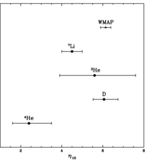
Fig. 1. The baryon density parameter, η10, inferred from SBBN and the relic abun-dances of D,3
He,4
He, and7
Li (filled circles), along with the non-BBN determination from WMAP (filled triangle). See the text for details.
If the standard model (SBBN) is the correct choice and if the primordial abundances inferred from the data were free of systematic errors, then the baryon densities determined from D,3He,4He, and7Li should agree among themselves and with that inferred from the CBR (WMAP) and other, non-BBN, cosmo-logical data. In Figure 1 are plotted the various values of the baryon density parameter1 determined by SBBN and the adopted primordial abundances and, also, from the WMAP-team analysis [2]. As may be seen from Fig. 1, the SBBN D abundance is in excellent agreement with the WMAP-inferred baryon den-sity. However, neither 7Li nor 4He agree with them or, even with each other. While 3He is consistent with SBBN deuterium and with WMAP (and is not in disagreement with7Li), the very large uncertainty in its primordial abundance, combined with its relative insensitivity to the baryon density, render it – at present – an even less sensitive baryometer than is4He.
In the next section each light nuclide is considered in turn, its post-BBN evolution briefly reviewed along with identification of a few of the potential challenges to accurately inferring the primordial abundances from the observa-tional data. Then, having established that the current data – taken at face value – are not entirely consistent with SBBN, I investigate whether changes in the early universe expansion rate can reconcile them.
2
Primordial Abundances – Evolution, Uncertainties,
Systematics
While Figure 1 suggests some problems with SBBN, the optimist may prefer to conclude that observations have provided impressive confirmation of the stan-dard cosmological model. After all, if the stanstan-dard model – or something very much like it – were not correct, there’d be no good reason why the abundances of four light nuclides, which range over some nine orders of magnitude, should be just such that the baryon densities inferred from each of them lie within a factor of three of each other, in nearly perfect agreement with that derived inde-pendently from non-BBN data. Only recently, when cosmology has entered an era of great precision, has it become important to distinguish accuracy from pre-cision and to revisit the path from precise astronomical observations to accurate abundances. For each of the light nuclides of interest here, an all too abbreviated overview of the current uncertainties is presented, with the intentional goal of creating controversey in order to stimulate future observations and theoretical analyses.
2.1 Deuterium
Deuterium is the baryometer of choice. During its post-BBN evolution, as gas is cycled through stars, D is only destroyed (setting aside rare astronomical events
1
Aftere±
annihilation during the early evolution of the Universe, the ratio of baryons to photons is, to a very good approximation, preserved down to the present. The baryon density parameter is defined to be this ratio (at present):η≡nN/nγ;η10≡ 1010
where, far from equilibrium, tiny amounts of D may be synthesized). Therefore, observations of D anywhere, at any time (e.g., the solar system or the local ISM), provide alower bound to its primordial abundance. As a result, it is ex-pected that observations of D in regions which have experienced minimal stellar evolution (e.g., the high redshift and/or low metallicity QSO Absorption Line Systems: QSOALS) should provide a good estimate of the relic abundance of deu-terium. Kirkmanet al.[3] have gathered the extant data; see [3] for details and related references. In Figure 2 are shown the QSOALS deuterium abundances as a function of metallicity; for reference, solar system and ISM D abundances are also shown.
While the observers are to be commended for their heroic work in identifying and analysing the tiny fraction of QSOALS which can be used to infer a low-metallicity, high redshift, D abundance, there are several unsettling aspects of the data displayed in Figure 1. Perhaps most noticeable is the paucity of data points. Without at all minimizing the difficulty of finding and analysing such systems, it is very nearly a sin to claim that the primordial abundance of a cosmologically key light nuclide is determined by five data points. If, however, the data points were in agreement within the estimated statistical errors, this might be less disturbing. It is clear from Fig. 1 that this is not the case. For these five data points the χ2 about the mean is >∼16, suggesting either that the uncertainties have been underestimated, or that some of these data may be contaminated by unidentified systematic errors. While the dispersion may
ISM
SUN
Fig. 2.The deuterium abundance (by number relative to hydrogen),yD≡10 5
(D/H), derived from high redshift, low metallicity QSOALS [3] (filled circles). The metallicity is on a log scale relative to solar; depending on the line-of-sight, X may be oxygen or silicon. Also shown is the solar system abundance (filled triangle) and that from observations of the local ISM (filled square).
simply be due to the small number of data points, it might be significant that the three QSOALS with the lower D/H ratios are LLS, while the two highest D/H determinations are from DLAs.
In the absence of evidence for changing or eliminating any of the current D abundance determinations, it is not unreasonable to follow the advice of [3] and adopt the weighted mean as an estimate of the primordial D abundance. Here, too, there is a (minor) problem. Kirkmanet al. [3] advocate finding the mean of log(D/H) to determine yD≡105(D/H);yD ≡10(5+<log(D/H)>)= 2.78. In contrast, if the weighted mean of the five D/H determinations is used,yD = 2.60. While this difference is well within the dispersion, it reflects the fact that in determining the mean of log(D/H), PKS1937 withyD = 3.24 dominates, while for the mean of D/H, HS0105 withyD= 2.54 dominates. In what follows I adopt yD = 2.6±0.4, where the error, following [3], is derived from the dispersion in D/H determinations. The corresponding BBN (SBBN) prediction for the baryon abundance,η10(D)≈6.1+0−0..75, is shown in Figure 1.
2.2 Helium-3
In my talk at this meeting I actually avoided discussion of3He, until it was forced upon me during the question session. In part, this was because this subject was ably covered in Tom Bania’s talk, in Dana Balser’s poster, and in Bob Rood’s conference summary. In part, however, it was because, in my opinion, for both observational and theoretical reasons3He has more to teach us about stellar and
Fig. 3. The 3
He abundances (by number relative to hydrogen), y3 ≡ 10 5
(3 He/H), derived from Galactic HII regions [4], as a function of galactocentric distance (filled circles). Also shown for comparison is the solar system abundance (solar symbol). The open circles are the oxygen abundances for the same HIIregions (and for the Sun).
Galactic evolution than about BBN. 3He is a less sensitive baryometer than is D since (D/H)BBN ∝ η−1.6, while (3He/H)BBN ∝η−0.6. Even more important is that, in contrast to the expected, monotonic, post-BBN evolution of D, the post-BBN evolution of3He is quite complicated, with competition between stel-lar production, destruction, and survival. For years, indeed decades, it had been anticipated that net stellar production would “win” and the abundance of3He would increase with time (and with metallicity); see,e.g., [5]. Unfortunately, ob-servations of3He are restricted to the solar system and the Galaxy. Nonetheless, since there is a clear galactic gradient of metallicity (see Fig. 3), a gradient in3He abundance would also be expected. If net production “wins”, then3He should be highest in the inner galaxy; the opposite if net destruction dominates. The ab-sence of any statistically significant gradient in the Bania, Rood, Balser (BRB) data [4] (see Fig. 3), points to an extremely delicate balance (cancellation) be-tween production and destruction. This suggests that the mean3He abundance in the Galaxy (y3≈1.9) might provide a reasonable estimate of the primordial abundance. However, BRB recommend that the 3He abundance determined in the most distant (from the Galactic center), most metal poor Galactic HIIregion yields an upper limit,y3<∼1.1±0.2, to the primordial abundance. The estimate ofη10(3He)≈5.6+2.0
−1.7 shown in Figure 1 is based on this choice. Had I adopted the mean value of y3 = 1.9, I would have inferredη10(3He) ≈ 2.3. While the former choice is in excellent agreement with deuterium (and with7Li and with the WMAP result [2]), the very large uncertainty renders 3He an insensitive baryometer; the latter option would be consistent with4He, but not with D (or with7Li or WMAP).
2.3 Helium-4
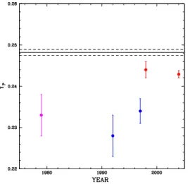
Helium-4 is the textbook example of a relic nuclide whose abundance is known precisely but, likely, inaccurately. To be of value in testing SBBN as well as in constraining non-standard models, YP should be determined to 0.001 or better. The largest uncertainty in the SBBN prediction is from the very small error in the neutron lifetime (τn = 885.7±0.7 s). For the WMAP estimate of the baryon
density, including its uncertainty, the SBBN-predicted primordial abundance is YP = 0.2482±0.0007, as shown in Figure 4. Also shown in Figure 4 is a record of YPdeterminations, from observations of extragalactic, low metallicity, HIIregions, covering the period from the late 1970s to the present (2004). During this time it has been well known, but often ignored, that there are a variety of systematic uncertainties which might dominate the YP determinations. In the hope of accounting for these systematic errors (rather than constraining them by observations), the error estimates for YP have often been inflated beyond the purely statsitical uncertainties. Thus, until the late 1990s, the typical error estimate for YP was 0.005. For example, summarizing the status as of 2000, Olive, Steigman, and Walker [7] suggested that the data available at that time were consistent with YP= 0.238±0.005; see Fig. 4. However, if4He were used as an SBBN baryometer (not recommended!), the error in the baryon density would have been ∼50%. Of course, as the number of HII regions observed increased,
largely due to the work of Izotov & Thuan [6], the statistical errors decreased. For example, from observations of 82 extragalactic HII regions, in their 2004 paper Izotov & Thuan quote [6] YP= 0.2429±0.0009; this data point is shown in Fig. 4. In contrast, a very recent, detailed study of the effects of some of the identified systematic uncertainties by Olive & Skillman [8] suggests the true errors are likely larger than this, by at least an order of magnitude.
As may be seen from Fig. 4, none of the YPestimates agree with the SBBN prediction, all being low by roughly 2-σ. Indeed, from their sample of 82 data points Izotov & Thuan [6] derive such a small uncertainty that their central value is low by nearly 6-σ. In their analysis, Izotov & Thuan commit the cardinal sin of examining their data and then,a posteriori, choosing a subsample of 7 HII re-gions to derive their favored estimate of YP= 0.2421±0.0021. One wonders what they may have found from a random series of choosing 7 of 82 data points. In any case, this estimate also falls short of the SBBN prediction by nearly 3-σ. Us-ing this suspect subsample, Olive & Skillman [8] do find consistency with SBBN once they have corrected for the systematic errors they’ve chosen to include. However, one they have ignored, the ionization correction factor [9], almost cer-tainly would have the effect of reducing their central value and increasing their error estimate. For the entire Izotov & Thuan sample, Olive & Skillman find a very large range for YP, from 0.232 to 0.258 (or, YP ≈0.245±0.013, entirely consistent with SBBN)). If the average correction for ionization suggested by Gruenwald, Steigman, and Viegas [9] for the somewhat smaller 1998 Izotov &
Fig. 4.A summary of the time evolution of primordial4
He abundance determinations (mass fraction YP) from observations of metal-poor, extragalactic HIIregions (see the text for references). The solid horizontal line is the SBBN-predicted 4
He abundance expected for the WMAP (and/or D) inferred baryon density. The two dashed lines show the 1σuncertainty in this prediction.
Thuan data set is applied to their 2004 compilation, it would suggest the Olive & Skillman central value be reduced and their error increased: YP≈0.239±0.015. If, indeed, the true uncertainty in YP is really this large, it opens the pos-sibility that there might be alternate approaches to YP which are competitive with the extragalactic, low-metallicity HII regions and, even more important, complementary in that they are subject to completely independent sets of sys-tematic errors. One such example, with a venerable history of its own, is to use effect of the initial helium abundance on the evolution of low-mass PopIIstars, employing the R-parameter [10]. Recently, Cassisi, Salaris, and Irwin [11] have attempted this using observations of a large sample of Galactic Globular Clus-ters (GGC) and new stellar models. While they claim an extraordinarily accurate determination of YP (0.243±0.006), this does not seem to be supported by the data they present since, for the lowest metallicity GGCs, Y ranges from<∼0.19 to >∼0.27. Nonetheless, if there is the possibility that the R-parameter method might achieve theoretical and observational uncertainties<∼0.01, it is certainly an approach worth pursuing.
An alternate approach, subject to large theoretical uncertainties, would be to attempt to use chemical evolution models, tied to the solar helium and heavy element abundances, to extrapolate back to the relic abundance of 4He. While at present this approach appears to be limited by the theoretical uncertainties (e.g., metallicity dependent stellar winds and stellar yields), the following ex-ample may serve as a stimulus (or challenge) to those who might believe they can do better. In a recent paper employing new yields, Chiappini, Matteucci, and Meynet [12] find ∆Y≡Y⊙−YP ≈0.018±0.006. Using the recent Bahcall
& Pinsonneault [13] estimate of Y⊙ ≈ 0.270±0.004, this leads to a
primor-dial estimate of YP ≈0.252±0.007. Although this result is consistent with the SBBN prediction, it would be entirely premature to declare victory on the basis of such a crude estimate. The possible lesson illustrated by this example is that the errorassociated with such an approach might not be uncompetitive with those from the standard HIIregion analyses.
2.4 Lithium-7
As with4He, the recent history of the comparison between the SBBN predictions and the observational data leading to the relic abundance of7Li is one of conflict, with the spectre of systematic errors looming large.7Li, along with6Li,9Be,10B, and 11B, is produced in the Galaxy by cosmic ray spallation/fusion reactions. Furthermore, observations of super-lithium rich red giants provide evidence that (some) stars are net producers of lithium. Therefore, to probe the BBN yield of 7Li, it is necessary to restrict attention to the most metal-poor halo stars (the “Spite plateau”). Using a specially selected data set of the lowest metallicity halo stars, Ryanet al.[14] claim evidence for a 0.3 dex increase in the lithium abundance ([Li] ≡12+log(Li/H)) for −3.5 ≤ [Fe/H] ≤ −1, and they derive a primordial abundance of [Li]P ≈ 2.0−2.1. This value is low compared to the estimate of Thorburn (1994) [15], who found [Li]P ≈ 2.25±0.10. In the
steps from the observed equivalent widths to the derived abundances, the stellar temperature plays a key role. When using the infrared flux method effective temperatures, studies of halo and Galactic Globular Cluster stars [16] suggest a higher abundance: [Li]P= 2.24±0.01. Very recently, Melendez & Ramirez [17] have reanalyzed 62 halo dwarfs using an improved infrared flux method effective temperature scale. They fail to find the [Li] vs. [Fe/H] gradient claimed by Ryan
et al.[14] and they confirm the higher lithium abundance, finding [Li]P= 2.37±
0.05. As shown in Figure 1, if this were the true primordial abundance of 7Li, thenη10(Li) = 4.5±0.4.Allof these observational determinations of primordial lithium are significantly lower than the SBBN expectation of [Li]P = 2.65+0−0..0506 for the WMAP baryon density.
As with4He, the culprit may be the astrophysics rather than the cosmology. Since the low metallicity, dwarf, halo stars used to constrain primordial lithium are the oldest in the Galaxy, they have had the most time to modify (by dilu-tion and/or destrucdilu-tion) their surface abundances. While mixing of the stellar surface material with the interior would destroy or dilute the prestellar lithium abundance, the very small dispersion in [Li] among the low metallicity halo stars suggests this effect may not be large enough to bridge the ≈ 0.3 dex gap be-tween the observed and WMAP/SBBN-predicted abundances ([Li]obs
P ≈ 2.37 versus [Li]predP ≈2.65); see,e.g., [18] and further references therein.
3
Non-Standard BBN
The path from acquiring observational data to deriving primordial abundances is long and complex and littered with pitfalls. While the predicted and observed relic abundances are in rough qualitative agreement, at present there exist some potential discrepancies. These may well be due to the data, the data analysis, or the extrapolations from here and now to there and then. But, there is also the possibility that these challenges to SBBN are providing hints of new physics beyond the standard models of particle physics and/or cosmology. Once this option is entertained, the possibilities are limited only by the imagination and creativity of physicists and cosmologists. Many such models have already been proposed and studied. One option is to discard most or all of standard physics and start afresh. A more conservative (not in the pejorative sense!) approach is to recognize that the standard model (SBBN) does quite well and to look for small variations on the same theme. Here, I’ll adopt the latter strategy and explore one such option which can resolve some, but not all, of the conflicts: a non-standard, early universe expansion rate.
There are many different extensions of the standard model of particle physics which result in modifications of the early universe expansion rate (the time – temperature relation). For example, additional particles will increase the energy density (at fixed temperature), resulting in a faster expansion. In such situations it is convenient to relate the extra energy density to that which would have been contributed by an additional neutrino with the ordinary weak interactions [19].
Just prior toe±annihilation, this may be written as
ρ′ ρ ≡1 +
7∆Nν
43 . (1)
Since the expansion rate (the Hubble parameter) depends on the square root of the combination of G (Newton’s contstant) and the density, the expansion rate factor (S) is related to∆Nν by,
S≡ H
′
H = (1 + 7∆Nν
43 )
1/2= (G′ G)
1/2
. (2)
Thus, while adding new particles (increasing the energy density) results in a speed-up in the expansion rate (∆Nν >0;S >1), changing the effective
New-ton’s constant may either increase or decrease the expansion rate. Another ex-ample of new physics which can alter the expansion rate is the late decay of a very massive particle which reheats the universe, but to a “low” reheat temper-ature [20]. If the reheat tempertemper-ature is too low (<∼7 MeV) the neutrinos will fail to be fully populated, resulting in ∆Nν < 0 and S < 1. Finally, in some
higher dimensional extensions of the standard model of particle physics addi-tional terms appear in the 3+1 dimensional Friedman equation whose behavior mimics that of “radiation”, resulting in an effective∆Nν which could be either
positive or negative [21].
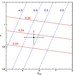
Fig. 5.Isoabundance curves for 4
He (solid) and D (dashed) in the baryon abundance (η10) – expansion rate factor (S) plane. The labels on the
4
He curves are for YP, while those on the D curves are foryD ≡10
5
(D/H). The filled circle with error bars corresponds to the adopted values of the D and4
He primordial abundances (see the text).
Thus, a nonstandard expansion rate (S6= 1) is a well-motivated, one param-eter modification of SBBN which has the potential to resolvesome of its chal-lenges. A slower expansion would leave more time for neutrons to become protons and a lower neutron abundance at BBN would result in a smaller YP (good!). Since4He is the most sensitive chronometer, the effect on its abundance is most significant. However, a modified expansion rate would also affect the predicted abundances of the other light nuclides as well. A slowdown will result in more destruction of D and 3He and, forη
10 >∼4, in production of more7Be (which becomes7Li via electron capture). In Figure 5 are shown the quite accurate ap-proximations to the isoabundance curves for D and YPin theS−η10plane, from the recent work of Kneller and myself [22]. Also shown in Fig. 5 is the location in this plane corresponding to the adopted D and4He abundances (including their uncertainties). Not surprisingly, it is possible to adjust these two parameters (S andη) to fit the relic abundances of these two nuclides. Note, however, that the best fit corresponds to aslower than standard expansion rate (S≈0.94±0.03; ∆Nν ≈ −0.70±0.35). While this combination of parameters is consistent with
WMAP (see,e.g., Barger et al. [23] and further references therein), it does not resolve the conflict with 7Li. Although a slowdown in the expansion rate does have the effect of increasing 7Li, this is compensated by the somewhat lower baryon density, which has the opposite effect. The result is that for these choices ofS andη, which do resolve the conflicts between D and4He (and WMAP and 4He), the predicted primordial abundance of7Li is still [Li]P≈2.62±0.10.
4
Summary and Conclusions
Four light nuclides (D, 3He, 4He, 7Li) are predicted to emerge from the early evolution of the universe in abundances large enough to be observed at present. In SBBN there is only one parameter, the baryon density parameter η, which determines the relic abundances of these nuclides. The current observational data identifies a range in this parameter of about a factor of 2-3 for which the SBBN predictions are in agreement with the primordial abundances inferred from current data. This range of η is also consistent with independent, non-BBN estimates [2]. Tests of the standard model of cosmology at 20 minutes (BBN) and nearly 400 thousand years later (WMAP) agree. While this is a great triumph for the standard models of cosmology and of particle physics, the agreement is not perfect and, if the uncertainty estimates are taken seriously, there are some challenges to this standard model. In this talk, to an audience of astronomers, I have emphasized the observational uncertainties in the hope of helping to stimulate further observational (and theoretical) work. Will more and better data resolve these apparent conflicts? Or, will we be pointed to new physics beyond the current standard models? Only time will tell.
Acknowledgments
It is with great pleasure that I express my thanks to the organizers of this very interactive and stimulating meeting, especially Luca Pasquini and Sofia Randich for their tireless efforts to facilitate my participation and to make it so enjoyable. The research described here has been supported at The Ohio State University by the US Department of Energy (DE-FG02-91ER40690).
References
1. G. Steigman: ‘Primordial Alchemy: From The Big Bang To The Present Universe’. In:Cosmochemistry: The Melting Pot of the Elements, XIII Canary Islands Winter School of Astrophysics, Tenerife, Canary Islands, Spain, November 19 – 30, 2001, ed. by C. Esteban, R.J. Garca L´opez, A. Herrero, & F. S´anchez (Cambridge Univer-sity Press, Cambridge 2004) p. 1; G. Steigman: ‘Big Bang Nucleosynthesis: Probing The First 20 Minutes’. In:Measuring and Modeling the Universe”, Carnegie Obser-vatories Astrophysics Series, Vol. 2, ed. by W.L. Freedman (Cambridge: Cambridge University Press 2004) p. 169
2. D.N. Spergel, et al.: ApJS,148, 175 (2003)
3. D. Kirkman, D. Tytler, N. Suzuki, J. O’Meara, D. Lubin: ApJS,149, 1 (2003) 4. T.M. Bania, R.T. Rood, D.S. Balser: Nature,415, 54 (2002)
5. R.T. Rood, G. Steigman, B.M. Tinsley, ApJ,207, L57 (1976)
6. J. Lequeux, M. Peimbert, J.F. Rayo, A. Serrano, S. Torres-Peimbert: A&A, 80, 155 (1979); B.E.J. Pagel, E.A. Simonson, R.J. Terlevich, M.G. Edmunds: MNRAS
255, 325 (1992); K.A. Olive, E.D. Skillman, G. Steigman: ApJ,489, 1006 (1997); Y.I. Izotov, T.X. Thuan: ApJ,500, 188 (1998);ibid, ApJ,602, 200 (2004) 7. K.A. Olive, G. Steigman, T.P. Walker: Phys. Rep.333, 389 (2000) 8. K.A. Olive, E.D. Skillman: astro-ph/0405588 (2004)
9. S.M. Viegas, R. Gruenwald, G. Steigman: ApJ,531, 813 (2000); R. Gruenwald, G. Steigman, S.M. Viegas: ApJ, 567, 931 (2002); D. Sauer, K. Jedamzik: A&A,
381, 361 (2002)
10. I. Iben: Nature220, 143 (1968)
11. S. Cassisi, M. Salaris, A.W. Irwin: ApJ,588, 862 (2003) 12. C. Chiappini, F. Matteucci, G. Meynet: A&A,410, 257 (2003) 13. J.N. Bahcall, M.H. Pinsonneault: Phys. Rev. Lett.92, 121301 (2004)
14. S.G. Ryan, J.E. Norris, T.C. Beers: ApJ,523, 654 (1999); S.G. Ryan, T.C. Beers, K.A. Olive, B.D. Fields, J.E. Norris: ApJ,530, L57 (2000)
15. J.A. Thorburn: ApJ,421, 318 (1994)
16. P. Bonifacio, P. Molaro: MNRAS, 285, 847 (1997); P. Bonifacio, P. Molaro, L. Pasquini: MNRAS,292, L1 (1997)
17. J. Melendez, I. Ramirez: ApJL,615, L33 (2004)
18. M.H. Pinsonneault, G. Steigman, T.P. Walker, V.K. Narayanan: ApJ, 574, 398 (2002)
19. G. Steigman, D.N. Schramm, J.E. Gunn: Phys. Lett. B66, 202 (1977)
20. M. Kawasaki, K. Kohri, N. Sugiyama: Phys. Rev. Lett.82, 4168 (1999); S. Hannes-tad: Phys. Rev. D70, 043506 (2004)
21. L. Randall, R. Sundrum: Phys. Rev. Lett.83, 3370 (1998);ibid, Phys. Rev. Lett.
83, 4690 (1998)
22. J.P. Kneller, G. Steigman: New J. Phys.6, 117 (2004)
23. V. Barger, J.P. Kneller, H.-S. Lee, D. Marfatia, G. Steigman: Phys. Lett. B566, 8 (2003)
![Fig. 2. The deuterium abundance (by number relative to hydrogen), y D ≡ 10 5 (D/H), derived from high redshift, low metallicity QSOALS [3] (filled circles)](https://thumb-us.123doks.com/thumbv2/123dok_us/8558862.2313422/4.918.332.590.599.866/deuterium-abundance-relative-hydrogen-derived-redshift-metallicity-qsoals.webp)
![Fig. 3. The 3 He abundances (by number relative to hydrogen), y 3 ≡ 10 5 ( 3 He/H), derived from Galactic H II regions [4], as a function of galactocentric distance (filled circles)](https://thumb-us.123doks.com/thumbv2/123dok_us/8558862.2313422/5.918.329.588.620.885/abundances-relative-hydrogen-derived-galactic-function-galactocentric-distance.webp)