Thomas G. Robertazzi
Stony Brook University September 19, 2011
Preface
Computer networking is a fascinating field that has interested many for quite a few years. The purpose of this brief book is to give a general, non-mathematical, introduction to the technology of networks. This includes discussions of types of communication, many networking standards, popular protocols, venues where net-working is important such as data centers, cloud computing and grid computing and the most important civilian encryption algorithm, AES.
This brief book can be used in undergraduate and graduate networking courses in universities or by the individual engineer, computer scientist or information tech-nology professional. In universities it can be used in conjunction with more mathe-matical modeling oriented texts.
I have learned a great deal about networking by teaching undergraduate and graduate courses on the topic at Stony Brook. I am grateful to Dantong Yu of Brookhaven National Laboratory for making me aware of many recent technological developments. Thanks are also due to Brett Kurzman, my editor at Springer, for supporting this brief book project. I would like to acknowledge the assistance in my regular duties at the university of my department’s superb staff of Gail Giordano, Carolyn Huggins, Rachel Ingrassia and Debbie Kloppenburg. I would also like to thank Prad Mohanty and Tony Olivo for excellent computer support.
The validation of my writing efforts by my daughters Rachel and Deanna and my good friend Sandy Pike means a lot. Finally I dedicate this brief book to the memory of my late wife and partner, Marsha.
1 Introduction to Networks 1
1.1 Introduction . . . 1
1.2 Achieving Connectivity . . . 2
1.2.1 Coaxial Cable . . . 2
1.2.2 Twisted Pair Wiring . . . 3
1.2.3 Fiber Optics . . . 4
1.2.4 Microwave Line of Sight . . . 5
1.2.5 Satellites . . . 5
1.2.6 Cellular Systems . . . 8
1.2.7 Ad Hoc Networks . . . 9
1.2.8 Wireless Sensor Networks . . . 11
1.3 Multiplexing . . . 12
1.3.1 Frequency Division Multiplexing (FDM) . . . 12
1.3.2 Time Division Multiplexing (TDM) . . . 13
1.3.3 Frequency Hopping . . . 14
1.3.4 Direct Sequence Spread Spectrum . . . 14
1.4 Circuit Switching Versus Packet Switching . . . 16
1.5 Layered Protocols . . . 18
2 Ethernet 23 2.1 Introduction . . . 23
2.2 10 Mbps Ethernet . . . 24
2.3 Fast Ethernet . . . 28
2.4 Gigabit Ethernet . . . 30
2.5 10 Gigabit Ethernet . . . 32
2.6 40/100 Gigabit Ethernet . . . 35
2.6.1 40/100 Gigabit Technology . . . 35
2.7 Conclusion . . . 37
3 InfiniBand 39 3.1 Introduction . . . 39
3.2 A First Look . . . 40
3.3 The InfiniBand Protocol . . . 41
3.4 InfiniBand for HPC . . . 42
4 Wireless Networks 45
4.1 Introduction . . . 45
4.2 802.11 WiFi . . . 45
4.2.1 The Original 802.11 Standard . . . 46
4.2.2 Other 802.11 Versions . . . 48
4.3 802.15 Bluetooth . . . 51
4.3.1 Technically Speaking . . . 52
4.3.2 Ad Hoc Networking . . . 53
4.3.3 Versions of Bluetooth . . . 53
4.3.4 802.15.4 Zigbee . . . 54
4.3.5 802.15.6 Wireless Body Area Networks . . . 56
4.3.6 Bluetooth Security . . . 57
4.4 802.16 Wireless MAN . . . 58
4.4.1 Introduction . . . 58
4.4.2 The Original 802.16 Standard . . . 59
4.4.3 More Recent 802.16 Standards . . . 60
4.4.4 802.16j . . . 62
4.4.5 802.16m . . . 63
4.5 LTE: Long Term Evolution . . . 64
4.5.2 LTE . . . 65
4.5.3 LTE Advanced . . . 66
5 Asynchronous Transfer Mode (ATM) 69 5.1 ATM (Asynchronous Transfer Mode) . . . 69
5.1.1 Limitations of STM . . . 70
5.1.2 ATM Features . . . 71
5.1.3 ATM Switching . . . 75
6 Multiprotocol Label Switching (MPLS) 79 6.1 Introduction . . . 79
6.2 Technical Details . . . 80
6.3 Traffic Engineering . . . 83
6.4 Fault Management . . . 84
6.5 GMPLS . . . 85
7 SONET and WDM 87 7.1 SONET . . . 87
7.1.1 SONET Architecture . . . 89
7.1.2 Self-Healing Rings . . . 92
7.2 Wavelength Division Multiplexing (WDM) . . . 94
8.1 Introduction . . . 97
8.2 Grids . . . 97
8.3 Cloud Computing . . . 101
8.3.1 Tradeoffs for Cloud Computing . . . 102
9 Data Centers 105 9.1 Introduction . . . 105
9.2 Data Centers . . . 106
9.2.1 Racks . . . 106
9.2.2 Networking Support . . . 106
9.2.3 Storage . . . 108
9.2.4 Electrical and Cooling Support . . . 108
9.2.5 Management Support . . . 110
9.2.6 Ownership . . . 110
9.2.7 Security . . . 110
10 Advanced Encryption Standard (AES) 111 10.1 Introduction . . . 111
10.2 DES . . . 112
10.3 Choosing AES . . . 112
10.4 AES Issues . . . 114
10.4.2 Performance Aspect . . . 115
10.4.3 Intellectual Property Aspect . . . 116
10.4.4 Some Other Aspects . . . 116
11 Bibliography 119
Introduction to Networks
1.1
Introduction
There is something about technology that allows people and their computers to com-municate with each other that makes networking a fascinating field, both technically and intellectually.
What is a network? It is a collection of computers (nodes) and transmission channels (links) that allow people to communicate over distances, large and small. A Bluetooth personal area network may simply connect your home PC with its peripherals. An undersea fiber optic cable may traverse an ocean. The Internet and telephone networks span the globe.
Networking in particular has been a child of the late twentieth century. The Internet has been developed over the past 40 years or so. The 1980’s and 1990’s saw the birth and growth of local area networks, SONET fiber networks and ATM back-bones. The 1990’s and the early years of the new century have seen the development and expansion of WDM fiber multiplexing. New wireless standards continue to ap-pear. Cloud computing and data centers are increasingly becoming a foundation of today’s networking/computing world.
The book’s purpose is to give a concise overview of some major topics in net-working. We now start with an introduction to the applied aspects of netnet-working.
1.2
Achieving Connectivity
A variety of transmission methods, both wired and wireless, are available today to provide connectivity between computers, networks, and people. Wired transmission media include coaxial cable, twisted pair wiring and fiber optics. Wireless technology includes microwave line of sight, satellites, cellular systems, ad hoc networks and wireless sensor networks. We now review these media and technologies.
1.2.1
Coaxial Cable
This is the thick cable you may have in your house to connect your cable TV set up box to the outside wiring plant. This type of cable has been around for many years and is a mature technology. While still popular for cable TV systems today, it was also a popular choice for wiring local area networks in the 1980s. It was used in the wiring of the original 10 Mbps Ethernet.
A coaxial cable has four parts: a copper inner core, surrounded by insulating material, surrounded by a metallic outer conductor; finally surrounded by a plastic outer cover. Essentially in a coaxial cable, there are two wires (copper inner core and outer conductor) with one geometrically inside the other. This configuration reduces interference to/from the coaxial cable with respect to other nearby wires.
The bandwidth of a coaxial cable is on the order of 1 GHz. How many bits per second can it carry? Modulation is used to match a digital stream to the spectrum carrying ability of the cable. Depending on the efficiency of the modulation scheme used, 1 bps requires anywhere from 1/14 to 4 Hz. For short distances, a coaxial cable may use 8 bits/Hz or carry 8 Gbps.
There are also different types of coaxial cable. One with a 50 ohm termination is used for digital transmissions. One with a 75 ohm termination is used for analog transmissions or cable TV systems.
A word is in order on cable TV systems. Such networks are locally wired as tree networks with the root node called the head end. At the head end, programming is brought in by fiber or satellite. From the head end cables (and possibly fiber) radiate out to homes. Amplifiers may be placed in this network when distances are large.
For many years, cable TV companies were interested in providing two way ser-vice. While early limited trials were generally not successful (except for Video on Demand), more recently cable TV seems to have winners in broadband access to the Internet and in carrying telephone traffic.
1.2.2
Twisted Pair Wiring
Coaxial cable is generally no longer used for wiring local area networks. One type of replacement wiring has been twisted pair. Twisted pair wiring typically had been previously used to wire phones to the telephone network. A twisted pair consists of two wires twisted together over their length. The twisted geometry reduces electromagnetic leakage (i.e. cross talk) with nearby wires. Twisted pairs can run several kilometers without the need for amplifiers. The quality of a twisted pair (carrying capacity) depends on the number of twists per inch.
About 1990, it became possible to send 10 Mbps (for Ethernet) over unshielded twisted pair (UTP). Higher speeds are also possible if the cable and connector pa-rameters are carefully implemented.
One type of unshielded twisted pair is category 3 UTP. It consists of four pairs of twisted pair surrounded by a sheath. It has a bandwidth of 16 MHz. Many offices used to be wired with category 3 wiring.
Category 5 UTP has more twists per inch. Thus, it has a higher bandwidth (100 MHz). Newer standards include category 6 versions (250 MHz or more) and category 7 versions (600 MHz or more). Category 8 at 1200 MHz is under development (Wikipedia).
The fact that twisted pair is lighter and thinner than coaxial cable has speeded its widespread acceptance.
1.2.3
Fiber Optics
Fiber optic cable consists of a silicon glass core that conducts light, rather than electricity as in coaxial cables and twisted pair wiring. The core is surrounded by cladding and then a plastic jacket.
Fiber optic cables have the highest data carrying capacity of any wired medium. A typical fiber has a capacity of 50 Tbps (terabits per second or 50×1012 bits per second). In fact, this data rate for years has been much higher than the speed at which standard electronics could load the fiber. This mismatch between fiber and nodal electronics speed has been called the electronic bottleneck. Decades ago the situation was reversed, links were slow and nodes were relatively fast. This paradigm shift has led to a redesign of protocols.
There are two major types of fiber: multi-mode and single mode. Pulse shapes are more accurately preserved in single mode fiber, lending to a higher potential data rate. However, the cost of multi-mode and single mode fiber is comparable. The real difference in pricing is in the opto-electronics needed at each end of the fiber. One of the reasons multi-mode fibers have a lower performance is dispersion. Under dispersion, square digital pulses tend to spread out in time, thus lowering the potential data rate. Special pulse shapes (such as hyperbolic cosines) called solitons, that dispersion is minimized for, have been the subject of research.
the fiber carries. Fusing two ends of the fiber results in a smaller attenuation.
Fiber optic cables today span continents and are laid across the bottom of oceans between continents. They are also used by organizations to internally carry tele-phone, data and video traffic.
1.2.4
Microwave Line of Sight
Microwave radio energy travels largely in straight lines. Thus, some network opera-tors construct networks of tall towers kilometers apart and place microwave antennas at different heights on each tower. While the advantage is that there is no need to dig trenches for cables, the expense of tower construction and maintenance must be taken into account.
1.2.5
Satellites
Arthur C. Clarke, the science fiction writer, made popular the concept of using satellites as communication relays in the late 1940s. Satellites are now extensively used for communication purposes. They fill certain technological niches very well: providing connectivity to mobile users, for large area broadcasts and for communi-cations for areas with poor infrastructure. The two main communication satellite architectures are geostationary satellites and low earth orbit satellites (LEOS). Both are now discussed.
Geostationary Satellites
You may recall from a physics course that a satellite in a low orbit (hundreds of kilometers) around the equator seems to move against the sky. As its orbital altitude increases, its apparent movement slows. At a certain altitude of approximately 36,000 km, it appears to stay in one spot in the sky, over the equator, 24 hours a
day. In reality, the satellite is moving around the earth but at the same angular speed that the earth is rotating, giving the illusion that it is hovering in the sky.
This is very useful. For instance, a satellite TV service can install home antennas that simply point to the spot in the sky where the satellite is located. Alternatively, a geostationary satellite can broadcast a signal to a large area (its footprint) 24 hours a day.
By international agreement, geostationary satellites are placed 2 degrees apart around the equator. Some locations are more economically preferable than others, depending on which regions of the earth are under the location.
A typical geostationary satellite will have several dozen transponders (relay am-plifiers), each with a bandwidth of 80 MHz (Tanenbaum 03). Such a satellite may weigh several thousand kilograms and consume several kilowatts using solar panels.
The number of microwave frequency bands used have increased over the years as the lower bands have become crowded and technology has improved. Frequency bands include L (1.5/1.6 GHz), S (1.9/2.2 GHz), C (4/6 GHz), Ku (11/14 GHz) and Ka (20/30 GHz) bands. Here the first number is the downlink band and the second number is the uplink band. The actual bandwidth of a signal may vary from about 15 MHz in the L band to several GHz in the Ka band (Tanenbaum 03).
It should be noted that extensive studies of satellite signal propagation under different weather and atmospheric conditions have been conducted. Excess power for overcoming rain attenuation is often budgeted above 11 GHz.
Low Earth Orbit Satellites
A more recent architecture is that of low earth orbit satellites. The most famous such system was Iridium from Motorola. It received its name because the original proposed 77 satellite network has the same number of satellites as the atomic number
North Pole
South Pole Polar
Orbit
Satellite
Earth
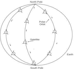
Figure 1.1: Low earth orbit satellites (LEOS) in polar orbits.
of the element Iridium. In fact, the actual system orbited had 66 satellites but the system name Iridium was kept.
The purpose of Iridium was to provide a global cell phone service. One would be able to use an Iridium phone anywhere in the world (even on the ocean or in the Artic). Unfortunately, after spending five billion dollars to deploy the system, talking on Iridium cost a dollar or more a minute while local terrestrial cell phone service was under 25 cents a minute. While an effort was made to appeal to business travelers, the system was not profitable and was sold and is now operated by a private company.
Technologically though, the Iridium system is interesting. There are eleven satel-lites in each of six polar orbits (passing over the North Pole, south to the South Pole and back up to the North Pole, see Figure 1.1).
At any given time, several satellites are moving across the sky over any location on earth. Using several dozen spot beams, the system can support almost a quarter of a million conversations. Calls can be relayed from satellite to satellite.
It should be noted that when Iridium was hot, several competitors were proposed but not built. One used a bent pipe architecture where a call to a satellite would be beamed down from the same satellite to a ground station and then sent over the terrestrial phone network rather than being relayed from satellite to satellite. This was done in an effort to lower costs and simplify the design.
1.2.6
Cellular Systems
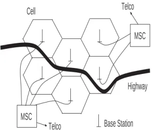
Starting around the early 1980s, cellular telephone systems which provide connectiv-ity between mobile phones and the public switched telephone network were deployed. In such systems, signals go from/to a cell phone to/from a local base station an-tenna which is hard wired into the public switched telephone network. Figure 1.2 illustrates such a system. A geographic region such as a city or suburb is divided into geographic sub-regions called cells.
Base stations are shown at the center of cells. Nearby base stations are wired into a switching computer (the mobile switching center or MSC) that provides a path to the telephone network.
A cell phone making a call connects to the nearest base station (i.e., the base station with the strongest signal). Base stations and cell phones measure and com-municate received power levels. If one is driving and one approaches a new base station, its signal will at some point become stronger than that of the original base station one is connected to and the system will then perform a handoff. In a hand-off, connectivity is changed from one base station to an adjacent one. Handoffs are transparent, the talking user is not aware when one occurs.
MSC
MSC
Highway
Telco
Telco
Base Station
Cell
Figure 1.2: Part of a cellular network.
called user’s phone.
The first cellular system was deployed in 1979 in Japan by NTT. The first U.S. cellular system was AMPS (Advanced Mobile Phone System) from AT&T. It was first deployed in 1983. These were first generation analog systems. Second gen-eration systems were digital. The most popular is the European originated GSM (Global System for Mobile), what has been installed over the world. Third and fourth generation cellular systems provide increased data rates for such applications as Internet browsing and picture transmission.
1.2.7
Ad Hoc Networks
Ad hoc networks (Murthy 04, Perkins 01) are radio networks where (often mobile) nodes can come together, transparently form a network without any user interaction
and maintain the network as long as the nodes are in range of each other and energy supplies last (Rabaey 00, Mauve 01). In an ad hoc network messages hop from node to node to reach an ultimate destination. For this reason ad hoc networks used to be called multi-hop radio networks. In fact, because of the nonlinear dependence of energy on transmission distance, the use of several small hops uses much less energy than a single large hop, often by orders of magnitude.
Ad hoc network characteristics include multi-hop transmission, possibly mobility and possibly limited energy to power the network nodes. Applications include mobile networks, emergency networks, wireless sensor networks and ad hoc gatherings of people, as at a convention center.
Routing is an important issue for ad hoc networks. Two major categories of routing algorithms are topology based routing and position based routing. Topology based routing uses information on current links to perform the routing. Position based routing makes use of a knowledge of the geographic location of each node to route. The position information may be acquired from a service such as the Global Positioning System (GPS).
Topology based algorithms may be further divided into proactive and reactive algorithms. Proactive algorithms use information on current paths as inputs to clas-sical routing algorithms. However to keep this information current a large amount of control message traffic is needed, even if a path is unused. This overhead problem is exacerbated if there are many topology changes (say due to movement of the nodes).
On the other hand, reactive algorithms such as DSR, TORA and AODV maintain routes only for paths currently in use to keep the amount of information and control overhead more manageable. Still, more control traffic is generated if there are many topology changes.
Position based routing does not require maintenance of routes, routing tables, or generation of large amounts of control traffic other than information regarding
positions. “Geocasting” to a specific area can be simply implemented. A number of heuristics can be used in implementing position based routing.
1.2.8
Wireless Sensor Networks
The integration of wireless, computer and sensor technology has the potential to make possible networks of miniature elements that can acquire sensor data and transmit the data to a human observer. Wireless sensor networks have received attention from researchers in universities, government and industry because of their promise to become a revolutionary technology and the technical challenges that must be overcome to make this a reality. It is assumed that such wireless sensor networks will use ad hoc radio networks to forward data in a multi-hop mode of operation.
Typical parameters for a wireless sensor unit (including computation and net-working circuitry) include a size from 1 millimeter to 1 centimeter, a weight less than 100 grams, cost less than one dollar and power consumption less than 100 mi-crowatts (Shah 02). By way of contrast, a wireless personal area network Bluetooth transceiver consumes more than a 1000 microwatts. A cubic millimeter wireless sensor can store, with battery technology, 1 Joule allowing a 10 microwatt energy consumption for 1 day (Kahn 00). Thus energy scavenging from light or vibration has been proposed. Note also that data rates are often relatively low for sensor data (100s bps to 100 Kbps).
Naturally, with these parameters, minimizing energy usage in wireless sensor networks becomes important. While in some applications wireless sensor networks may be needed for a day or less, there are many applications where a continuous source of power is necessary. Moreover, communication is much more energy expen-sive than computation. Sending one bit for a distance of 100 meters can take as much energy as processing 3000 instructions on a micro-processor.
are many potential scientific and civilian applications of wireless sensor networks. Scientific applications include geophysical, environmental and planetary exploration. One can imagine wireless sensor networks being used to investigate volcanoes, mea-sure weather, monitor beach pollution or record planetary surface conditions.
Biomedical applications include applications such as glucose level monitoring and retinal prosthesis (Schwiebert 01). Such applications are particularly demanding in terms of manufacturing sensors that can survive in and not affect the human body.
Sensors can be placed in machines (where vibration can sometimes supply en-ergy) such as rotating machines, semiconductor processing chambers, robots and engines. Wireless sensors in engines could be used for pollution control telemetry.
Finally, among many potential applications, wireless sensors could be placed in homes and buildings for climate control. Note that wiring a single sensor in a building can cost several hundred dollars. Ultimately, wireless sensors could be embedded in building materials.
1.3
Multiplexing
Multiplexing involves sending multiple signals over a single medium. Thomas Edison invented a four to one telegraph multiplexer that allowed four telegraph signals to be sent over one wire. The major forms of multiplexing for networking today are frequency division multiplexing (FDM), time division multiplexing (TDM) and spread spectrum. Each is now reviewed.
1.3.1
Frequency Division Multiplexing (FDM)
Here a portion of spectrum (i.e. band of frequencies) is reserved for each channel (Figure 1.3(a)). All channels are transmitted simultaneously but a tunable filter at
slot 1 slot 2 slot 3 slot N slot 1 slot 2
Frame 1 Frame 2
FDM
TDM (a)
(b)
channel 1 channel 2 channel 3 channel N frequency
time
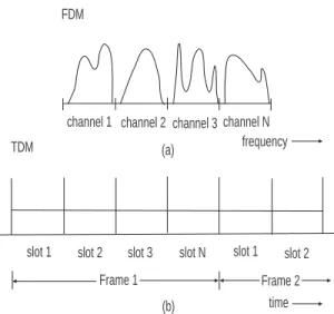
Figure 1.3: (a) Frequency division multiplexing, (b) Time division multiplexing.
the receiver only allows one channel at a time to be received. This is how AM, FM and analog television signals are transmitted. Moreover, it is how distinct optical signals are transmitted over a fiber using wavelength division multiplexing (WDM) technology.
1.3.2
Time Division Multiplexing (TDM)
Time division multiplexing is a digital technology that, on a serial link, breaks time into equi-duration slots (Figure 1.3(b)). A slot may hold a voice sample in a telephone system or a packet in a packet switching system. A frame consists of N slots. Frames, and thus slots, repeat. A telephone channel might use slot 14 of 24 slots in a frame during the length of a call, for instance.
It is also used in digital telephone switches. Such switches in fact use electronic devices called time slot interchangers that transfer voice samples from one slot to another to accomplish switching.
1.3.3
Frequency Hopping
Frequency hopping is one form of spread spectrum technology and is typically used on radio channels. The carrier (center) frequency of a transmission is pseudo-randomly hopped among a number of frequencies. (Figure 1.4(a)). The hopping is done in a deterministic, but random looking pattern that is known to both trans-mitter and receiver. If the hopping pattern is known only to the transtrans-mitter and receiver, one has good security. Frequency hopping also provides good interference rejection. Multiple transmissions can be multiplexed in the same local region if each uses a sufficiently different hopping pattern. Frequency hopping dates back to the era of World War II.
1.3.4
Direct Sequence Spread Spectrum
This alternative spread spectrum technology uses exclusive or (xor) gates as scram-blers and de-scramscram-blers. (Figure 1.4(b)). At the transmitter data is fed into one input of an xor gate and a pseudo-random key stream into the other input.
Table 1.1: XOR Truth Table Key Data Output
0 0 0
0 1 1
1 0 1
1 1 0
From the xor truth table, one can see that if the key bit is a zero, the output bit equals the data bit. If the key bit is a one, the output bit is the complement of the data bit (0 becomes 1, 1 becomes 0). This scrambling action is quite strong
f f f f 1 2 3 4 time Frequency Hopping (a) XOR 1 0 1 0 0 Key stream XOR 1 0 1 0 0 Key stream Channel Transmitter Receiver Direct Sequence Data Data 00110 00110 (b)
Figure 1.4: (a) Frequency hopping spread spectrum, (b) Direct sequence spread spectrum.
under the proper conditions. Unscrambling can be performed by an xor gate at the receiver. The transmitter and receiver must use the same (synchronized) key stream for this to work. Again, multiple transmissions can be multiplexed in a local region if the key streams used for each transmission are sufficiently different.
1.4
Circuit Switching Versus Packet Switching
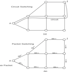
Two major architectures for networking and telecommunications are circuit switch-ing and packet switchswitch-ing. Circuit switchswitch-ing is the older technology, goswitch-ing back to the years following the invention of the telephone in the late 1800’s. As illustrated in Figure 1.5(a), for a telephone network, when a call has to be made from node A to node Z, a physical path with appropriate resources called a circuit is established. Resources include link bandwidth and switching resources. Establishing a circuit requires some set-up time before actual communication commences. Even if one momentarily stops talking, the circuit is still in operation. When the call is fin-ished, link and switching resources are released for use by other calls. If insufficient resources are available to set up a call, the call is said to be blocked.
Packet switching was created during the 1960’s. A packet is a bundle of bits consisting of header bits and payload bits. The header contains the source and des-tination address, priority levels, error check bits and any other information that is needed. The payload is the actual information (data) to be transported. However, many packet switching systems have a maximum packet size. Thus, larger trans-missions are split into many packets and the transmission is reconstituted at the receiver.
The diagram of Figure 1.5(b) shows packets, possibly from the same transmis-sion, taking multiple routes from node A to node Z. This is called datagram or connectionless oriented service. Packets may indeed take different routes in this type of service as nodal routing tables are updated periodically in the middle of a
(a)
(b) circuit A
Z
A
Z Circuit Switching
Packet Switching
Packet
Figure 1.5: (a) Circuit switching, (b) Packet switching.
transmission.
A hybrid type of service is the use of virtual circuits or connection oriented service. Here packets belonging to the same transmission are forced to take the same serial path through the network. A virtual circuit has an identification number which is used at nodes to continue the circuit along its preset path. As in circuit switching, a virtual circuit needs to be set up prior to its use for communication. That is, entries need to be made in routing tables implementing the virtual circuit.
An advantage of virtual circuit usage is that packets arrive at the destination in the same order that they were sent. This avoids the need for buffers for reassembling transmissions (reassembly buffers) that are needed when packets arriving at the destination are not in order, as in datagram service. As we shall see, ATM, the high speed packet switching technology used in Internet backbones, uses virtual circuits.
Packet switching is advantageous when traffic is bursty (occurs at irregular in-tervals) and individual transmissions are short. It is a very efficient way of sharing network transmissions when there are many such transmissions. Circuit switching is not well suited for bursty and short transmissions. It is more efficacious when transmissions are relatively long (to minimize set up time overhead) and provide a constant traffic rate (to well utilize the dedicated circuit resource).
1.5
Layered Protocols
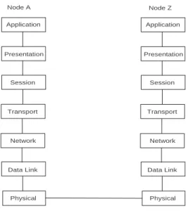
Protocols are the rules of operation of a network. A common way to engineer a complex system is to break it into more manageable and coherent components. Network protocols are often divided into layers in the layered protocol approach. Figure 1.6 illustrates the generic OSI (open systems interconnection) protocol stack. Proprietary protocols may have different names for the layers and/or a different layer organization but pretty much all networking protocols have the same functionality.
Transmissions in a layered architecture (see Figure 1.6) move from the source’s top layer (application), down the stack to the physical layer, through a physical channel in a network, to the destination’s physical layer, up the destination stack to the destination application layer. Note that any communication between peer layers must move down one stack, across and up the receiver’s stack. It should also be noted that if a transmission passes through an intermediate node, only some lower layers (e.g., network, data link and physical) may be used at the intermediate nodes.
It is interesting that a packet moving down the source’s stack may have its header grow as each layer may append information to the layer. At the destination, each layer may remove information from the packet header, causing it to decrease in size as it moves up the stack.
In a particular implementation, some layers may be larger and more complex while others are relatively simple.
Application
Presentation
Session
Transport
Network
Data Link
Physical Application
Presentation
Session
Transport
Network
Data Link
Physical
Node A Node Z
Figure 1.6: OSI protocol stack for a communicating source and destination.
In the following, we briefly discuss each layer.
Application Layer
Applications for networking include email, remote login, file transfer and the world-wide web. But an application may also be more specialized, such as distributed software to run a network of catalog company order depots.
Presentation Layer
This layer controls how information is formatted, such as on a screen (number of lines, number of characters across).
Session Layer
This layer is important for managing a session, as in remote logins. In other cases, this is not a concern.
Transport Layer
This layer can be thought of as an interface between the upper and lower layers. More importantly, it is designed to give the impression to the layers above that they are dealing with a reliable network, even though the layers below the transport layer may not be perfectly reliable. For this reason, some think of the transport layer as the most important layer.
Network Layer
The network layer manages multiple links. Its most important function is to do routing. Routing involves selecting the best path for a circuit or packet stream.
Data Link Layer
Whereas, the network layer manages multiple link functions, a data link protocol manages a single link. One of its potential functions is encryption, which can either be done on a link by link basis (i.e. at the data link layer) or on an end to end basis (i.e. at the transport layer) or both. End to end encryption is a more conservative choice as one is never sure what type of sub-network a transmission may pass thru and what its level of encryption, if any, is.
Physical Layer
The physical layer is concerned with the raw transmission of bits. Thus, it includes engineering physical transmission media, modulation and de-modulation and radio technology. Many communication engineers work on physical layer aspects of net-works. Again, the physical layer of a protocol stack is the only layer that provides actual direct connectivity to peer layers.
Ethernet
2.1
Introduction
Local area networks (LANs) are networks that cover a small area as in a department in a company or university. In the early 1980s, the three major local area networks were Ethernet (IEEE standard 802.3), Token Ring (802.5 and used extensively by IBM) and Token Bus (802.4, intended for manufacturing plants). However, over the years, Ethernet (Tanenbaum 03) has become the most popular local area network standard. While maintaining a low cost, it has gone through six versions, most ten times faster than the previous version (10 Mbps, 100 Mbps, 1 Gbps, 10 Gbps, 40 Gbps, 100 Gbps).
Ethernet was invented at the Xerox Palo Alto Research Center (PARC) by Met-calfe and Boggs, circa 1976. It is similar in spirit to the earlier Aloha radio protocol, though the scale is smaller. IEEE’s 802.3 committee produced the first Ethernet standard. Xerox never produced Ethernet commercially but other companies did.
In going from one Ethernet version to the next, the IEEE 802.3 committee sought to make each version similar to the previous ones and to use existing technology. In the following, we now discuss the various versions of Ethernet.
Coaxial Cable
Computers
(a)
Hub
Computers
(b)
To Backbone
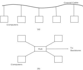
Figure 2.1: Ethernet wiring using (a) coaxial cable and (b) hub topology.
2.2
10 Mbps Ethernet
Back in the 1980’s, Ethernet was originally wired using coaxial cable. As in Fig-ure 2.1(a), a coaxial cable was snaked through the floor or ceiling and computers attached to it along its length. The coaxial cable acted as a private radio channel that each computer would monitor. If a station had a packet to send, it would send it immediately if the channel was idle. If the station sensed the channel to be busy, it would wait until the channel was free. In all of this, only one transmission can be on the channel at one time.
A problem occurs if two or more stations sense the channel to be idle at about the same time and attempt to transmit simultaneously. The packets overlap in the cable and are garbled. This is a collision. The stations involved, using analog electronics, can detect the collision, stop transmitting and reschedule their transmissions.
Thus, the price one pays for this completely decentralized access protocol is the presence of utilization lowering collisions. The protocol used goes by the name 1-persistent CSMA/CD (Carrier Sense Multiple Access with Collision Detection). The name is pretty much self-explanatory except that 1-persistent refers to the fact that a station with a packet to send attempts this on an idle channel with a probability of 1.0. In a CSMA/CD protocol, if the bit rate is 10 Mbps, the actual useful information transport can be significantly less because of collisions (or occasional idleness).
In the case of a collision, the rescheduling algorithm used is called Binary Expo-nential Backoff. Under this protocol, two or more stations experiencing a collision randomly reschedule over a time window with a default of 51 microseconds for a 500 meter network. If a station becomes involved in a second collision, it doubles its window size and attempts again to randomly reschedule its transmission. Windows may be doubled in size up to ten times. Once a packet is successfully transmit-ted, the window size drops back to the default (smallest) value for that packet’s station. Thus, this protocol at a station has no long term memory regarding past transmissions.
Table 2.1: Ethernet Frame Format Field Length
Preamble 7 bytes Frame Delimiter 1 byte Destination Address 2 or 6 bytes Source Address 2 or 6 bytes Data Length 2 bytes
Data up to 1500 bytes Pad variable
CRC Checksum 4 bytes
Table 2.1 above shows the fields in the 10 Mbp Ethernet frame. A frame is the name for a packet at the data link layer. The preamble is for communication receiver synchronization purposes. Addresses are either local (2 bytes) or global (6 bytes).
Note that Ethernet addresses are different from IP addresses. Different amounts of data can be accommodated up to 1500 bytes. Transmissions longer than 1500 bytes of data must be segmented into multiple packets. The pad field is used to guarantee that the frame is at least 64 bytes in length (minimum frame size) if the frame would be less than 64 bytes in length. Finally the checksum is based on CRC error detecting coding.
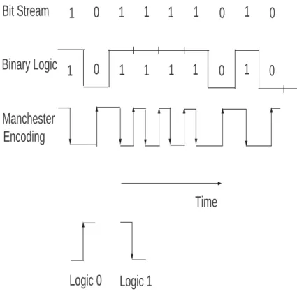
A problem with digital receivers is that they require many 0 to 1 and 1 to 0 transitions to properly lock onto a signal. But long runs of 1’s or 0’s are not uncommon in data. To provide many transitions between logic levels, even if the data has a long run of one logic level, 10 Mbps Ethernet uses Manchester encoding.
Referring to Figure 2.2, under Manchester encoding, if a logic 0 needs to be sent, a transition is made for 0 to 1 (low to high voltage) and if a logic 1 needs to be sent, the opposite transition is made for 1 to 0 (high to low voltage). The voltage level makes a return to its original level at the end of a bit as necessary. Note that the signaling rate is variable. That is, the number of transitions per second is twice the data rate for long runs of a logic level and is equal to the data rate if the logic level alternates. For this reason, Manchester encoding is said to have an efficiency of 50%. More modern signaling codes, such as 4B5B, achieve a higher efficiency (see Fast Ethernet below).
During the 1980s, Ethernets were wired with linear coaxial cables. Today hubs are commonly used (Figure 2.1(b)). These are boxes (some smaller than a cigar box) that computers tie into, in a star type wiring pattern, with the hub at the center of the star.
A hub may internally have multiple cards, each of which have multiple external Ethernet connections. A high speed (in the gigabits) proprietary bus interconnects the cards. Cards may mimic a CSMA/CD Ethernet with collisions (shared hub) or use buffers at each input (switched hub). In a switched hub, multiple packets may be received simultaneously without collisions, raising throughput.
1
0
1
1
1
1
0
1
0
1
0
1
1
1
1
0
1
0
Time
Bit Stream
Binary Logic
Manchester
Encoding
Logic 0
Logic 1
The next table (Table 2.2) illustrates Ethernet wiring. In 10 Base5, the 10 stands for 10 Mbps and the 5 for the 500 meter maximum size. Used in the early 1980s, 10 Base5 used vampire taps which would puncture the cable. Also at the time, 10 Base2 used T junctions and BNC connectors as wiring hardware. Today, 10 Base-T is the most common wiring solution for 10 Mbps Ethernet. Fiber optics, 10 Base-F, is only intended for runs between buildings, but a higher data rate protocol would probably be used today for this purpose.
Table 2.2: Original Ethernet Wiring Cable Type Maximum Size 10Base5 Thick Coax 500 m
10Base2 Thin Coax 200 m 10Base-T Twisted Pair 100 m 10Base-F Fiber Optics 2 km
2.3
Fast Ethernet
As the original 10 Mbps Ethernet became popular and the years passed, traffic on Ethernet networks continued to grow. To maintain performance, network ad-ministrators were forced to segment Ethernet networks into smaller networks (each handling a smaller number of computers) connected by a spaghetti-like arrangement of repeaters, bridges and routers. In 1992, IEEE assigned the 802.3 committee the task of developing a faster local area network protocol.
The committee agreed on a 100 Mbps protocol that would incorporate as much of the existing Ethernet protocol/technology as possible to gain acceptance and so that they could move quickly. The resulting protocol, IEEE 802.3u, was called Fast Ethernet.
Fast Ethernet is only implemented with hubs, in a star topology (Figure 2.1(b)). There are three major wiring options (Table 2.3).
Table 2.3: Fast Ethernet Wiring Cable Type Maximum Size 100Base-T4 Twisted Pair 100 m
100Base-TX Twisted Pair 100 m 100Base-FX Fiber Optics 2 km
The original Ethernet has a data rate of 10 Mbps and a maximum signaling rate of 20 MHz (recall that the Manchester encoding used was 50% efficient). Fast Ethernet 100 Base-T4 with its data rate of 100 Mbps has a signaling speed of 25 MHz, not 200 MHz. How is this accomplished?
Fast Ethernet 100 Base-T4 actually uses four twisted pairs per cable. Three twisted pairs carry signals from its hub to a PC. Each of the three twisted pairs uses ternary (not binary) signaling using 3 logic levels. Thus, one of 3x3x3=27 symbols can be sent at once. Only 16 symbols are used though, which is equivalent to sending 4 bits at once. With 25 MHz clocking 25 MHz x 4 bits yields a data rate of 100 Mbps. The channel from the PC to hub operates at 33 MHz. For most PC applications, an asymmetrical connection with more capacity from hub to PC for downloads is acceptable. Category 3 or 5 unshielded twisted pair wiring is used for 100 Base-T4.
An alternative to 100 Base-T4 is 100 Base-TX. This uses two twisted pairs, with 100 Mbps in each direction. However, 100 Base-T4 has a signaling rate of only 125 MHz. It accomplishes this using 4B5B (Four Bit Five Bit) encoding rather than Manchester encoding. Under 4B5B, every four bits is mapped into five bits in such a way that there are many transitions for digital receivers to lock onto, irrespective of the actual data stream. Since four bits are mapped into five bits, 4B5B is 80% efficient. Thus, 125 MHz times 0.8 yields 100 Mbps.
Finally, 100 Base-FX uses two strands of the lower performing multimode fiber. It has 100 Mbps in both directions and is for runs (say between buildings) of up to 2 km.
It should be noted that Fast Ethernet uses the signaling method for twisted pair (for 100 Base-TX) and fiber (100 Base-FX) borrowed from FDDI. The FDDI protocol was a 100 Mbps token ring protocol used as a backbone in the 1980’s.
To maintain channel efficiency (utilization) at 100 Mbps, versus the original 10 Mbps, the maximum network size of Fast Ethernet is about ten times smaller than that of the original Ethernet.
2.4
Gigabit Ethernet
The ever growing amount of network traffic brought on by the growth of applica-tions and more powerful computers motivated a revised, faster version of Ethernet. Approved in 1998, the next version of Ethernet operates at 1000 Mbps or 1 Gbps and is known as Gigabit Ethernet, or 802.3z. As much as possible, the Ethernet committee sought to utilize existing Ethernet features.
Gigabit Ethernet wiring is either between two computers directly or, as is more common, in a star topology with a hub or switch in the center of the star. In this connection, it is appropriate to say something about the distinction between a hub and switch. A shared medium hub uses the established CSMA/CD protocol so collisions can occur. At most, one attached station can successfully transmit through the hub at a time, as one would expect with CSMA/CD. The half duplex Gigabit Ethernet mode uses shared medium hubs.
A switch on the other hand, does not use CSMA/CD. Rather, the use of buffers means multiple attached stations may send and receive distinct communications to/from the switch at the same time. The use of multiple simultaneous transmissions means that switch throughput is substantially greater than that of a single input line. Level 2 switches are usually implemented in software, level 3 switches implement routing functions in hardware (Stallings 02). Full duplex Gigabit Ethernet most often uses switches.
In terms of wiring, Gigabit Ethernet has two fiber optic options (1000 Base-SX and 1000 Base-LX), a copper option (1000 Base-CX) and a twisted pair option (1000-Base T).
The Gigabit Ethernet fiber option deserves some comment. It makes use of 8B10B encoding, which is similar in its operation to Fast Ethernet’s 4B5B. Under 8B10B, eight bits (1 byte) are mapped into 10 bits. The extra redundancy this involves allows each 10 bits not to have an excessive number of bits of the same type in a row or too many bits of one type in each of 10 bits. Thus, there are sufficient transitions from 1 to 0 and 0 to 1 or the data stream even if the data has a long run of 1s and 0s.
Gigabit Ethernet using twisted pair uses five logic levels on each wire. Four of the logic levels convey data and the fifth is for control signaling. With four data logic levels, two bits are communicated at once or eight bits over all four wires at a time. Thus the signaling rate is 1 Gbps/8 or 125 MHz.
In terms of utilization under CSMA/CD operation, if the maximum segment size had been reduced by a factor of 10 as was done in going from the original Ethernet to Fast Ethernet, only very small gigabit networks could have been supported. To compensate for the ten times increase in data rate relative to Fast Ethernet, the minimum frame size for Gigabit Ethernet was increased (by a factor of eight) to 512 bytes from Fast Ethernet’s 512 bits (see Robertazzi 07 for a discussion of the Ethernet equation that governs this).
Another technique that helps Gigabit Ethernet’s efficiency is frame bursting. Under frame bursting, a series of frames are sent in a single burst.
Gigabit Ethernet’s range is at least 500 meters for most of the fiber options and about 200 meters for twisted pair (Tanenbaum 03, Stallings 02).
2.5
10 Gigabit Ethernet
Considering the improvement in Ethernet data rate over the years, it is not too surprising that a 10 Gbps Ethernet was developed (Siwamogsatham 99, Vaughan-Nichols 02). Continuing the increases in data rate by a factor of ten that have characterized the Ethernet standards, 10 Gbps (or 10,000 Mbps) Ethernet is ten times faster than Gigabit Ethernet. Applications include backbones, campus size networks and metropolitan and wide area networks. This latter application is aided by the fact that the 10 Gbps data rate is comparable with a basic SONET fiber optic transmission standard rate. In fact, 10 Gbps Ethernet will be a competitor to ATM high speed packet switching technology. See the following chapters for more information on ATM and SONET.
There are eight implementations of 10 Gbps Ethernet. It can use four transceiver types (one four wavelength parallel system and three serial systems with a number of multimode and single mode fiber options). Like earlier versions of Ethernet, it uses CRC error coding. It operates in full duplex non-CSMA/CD mode. It can go more than 40 km via single mode fiber.
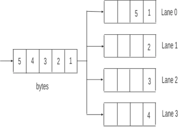
To lower the speed at which the MAC (Media Access Control) layer processes the data stream, the MAC operates in parallel on four 2.5 Gbps streams (lanes). As illustrated in Figure 2.3, bytes in an arriving 10 Gbps serial transmission are placed in parallel in the four lanes.
There is a 12 byte Inter Packet Gap (IPG) which is the minimum gap between packets. Normally, it would not be easy to predict the ending byte lane of the previous packet, so it would be difficult to determine the starting lane of the next transmission. The solution is to have a starting byte in a packet always occupy lane 0. The IPG is found using a pad (add in extra 1 to 3 bytes), a shrink (subtract 1 to 3 bytes) or through combination averaging (average of 12 bytes achieved through a combination of pads and shrinks). Note that padding introduces extra overhead in
1 2 3 4 5
1
2
3
4 5 Lane 0
Lane 1
Lane 2
Lane 3 bytes
Figure 2.3: Four parallel lanes for 10 Gigabit Ethernet.
some implementations.
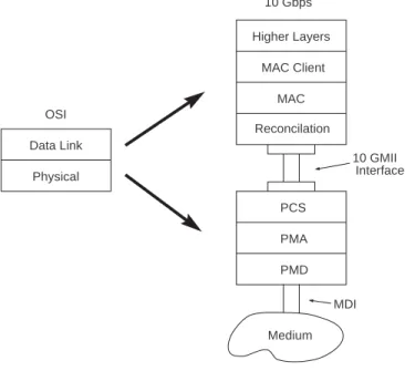
In terms of the protocol stack, this can be visualized as in Fig. 2.4.
The PCS, PMA and PMD sub-layers use parallel lanes for processing. In terms of the sub-layers, they are:
Reconciliation: Command translator that maps terminology and commands in MAC into electrical format appropriate for physical layer.
PCS: Physical Coding Sublayer.
PMA: Physical Medium Attachment (at transmitter serialize code groups into bit stream, at receiver synchronization for data decoding).
PMD: Physical Medium Dependent (includes amplification, modulation, wave shaping).
Reconcilation Higher Layers MAC Client
MAC 10 Gbps
OSI Data Link
Physical
PCS PMA PMD
Medium
10 GMII Interface
MDI
2.6
40/100 Gigabit Ethernet
Over the years Ethernet has been attractive to users because of its relatively low cost, robustness and its ability to provide an interoperable network service. Users have also liked the wide vendor availability of Ethernet related products. However even with the release of gigabit and 10 Gbps Ethernet demand for bandwidth continued to grow. Network equipment shipments can grow at a 17% a year rate. Internet traffic grows at 75-125% a year. Computer performance doubles every 24 months. A 2008 projection was that within four years 40 Gbps would be needed.
One of the applications driving this growth is the increasing use of data centers (see the latter chapter on this topic). These facilities house server farms for hosting web services and cloud computing services. Projections indicate a need for 100 Gbps of data transfer capacity from switch to switch. Also 100 Gbps will have applications between buildings, within campuses and for metropolitan area networks (MAN) and wide area networks (WAN).
In July 2006 a committee was convened to explore increasing the data rate of Ethernet beyond 10 Gbps. In 2010 standards for 40 Gbps and 100 Gbps Ethernet were approved. This discussion is based on (D’Ambrosia 2008, Nowell 2007).
2.6.1
40/100 Gigabit Technology
In implementing 40 and 100 gigabit Ethernet some of the objectives are:
· MAC (medium access control) data rates of 40 and 100 gigabit per second.
· Full duplex is only supported (i.e. two way communication).
· Maintain the existing minimum and maximum frame length.
MAC Client
MAC Control (optional) MAC Reconciliation PCS FEC (option) PMA PMD AN (option) Medium
40 Gbps 100 Gbps
MDI PCS FEC (option) PMA PMD AN (option) Medium MDI
Figure 2.5: 40 and 100 Gbps Ethernet protocol functions
· Optical transport network (OTN) support.
A variety of transmission media can carry 40 and 100 gigabit Ethernet as Table 2.4 illustrates.
Table 2.4: 40/100 Gbps Ethernet 40 Gbps 100 Gbps
≥ 10 km Single Mode Fiber ≥ 40 km Single-Mode Fiber
≥ 100 m Multi-mode Fiber ≥ 10 km Single Mode Fiber
≥ 10 m Copper cable ≥ 100 m Multi-mode Fiber
≥ 1 m Backplane ≥ 10 m Copper Cable
Figure 2.5 illustrates the protocol stack for 40 and 100 gigabit Ethernet. In the figure one has the physical coding sublayer (PCS), the forward error correction sublayer (FEC), physical medium attachment sublayer (PMA), physical medium dependent sublayer (PMD) and the auto-negotiation sublayer (AN). Here also MDI is the medium dependent interface or the connector.
In the physical coding sublayer 64B/66B coding is used, mapping 64 bits into 66 bits to provide enough transitions between 0 and 1 for digital receivers. As in 10 gigabit Ethernet, the concept of parallel lanes is used in 40 and 100 gigabit Ethernet. A 66 bit block is distributed in round robin fashion on the PCS lanes. Specifically for 40 gigabit Ethernet there are 4 PCS lanes that support 1 2 or 4 channels or wavelengths. For 100 gigabit Ethernet there are 20 PCS lanes that support 1, 2, 4, 5, 10, or 20 channels or wavelengths. As an example, a 100 gigabit Ethernet may use 5 parallel wavelengths over a fiber, each carrying 20 Gbps.
Created PCS lanes can be multiplexed into any interface width that is supported. There is a unique lane marker for each PCS lane which is inserted perioidically. Bandwidth for the lane marker comes from periodically deleting the inter-packet gap (IPG) in a lane. All bits in the same lane follow the same physical path no matter how multiplexing is done.
The receiver reassembles the PCS lanes by demultiplexing bits and also realigns the PCS lanes taking into account the skewness of the lanes. Advantages of this include the fact that all encoding, deskew and scrambling functions are implemented on a CMOS device located on the host and there is minimal bit processing execept for using an optical module for multiplexing.
Finally, clocking takes place at 1/64th of the data rate (625 MHz for 40 gigabits and 1.5625 GHz for 100 gigabits). More information on 40 and 100 gigabit Ethernet can be found on www.ethernetalliance.org
2.7
Conclusion
For thirty years Ethernet has continually transformed itself by way of higher data rates to meet increasing demand for networking services. It will be interesting to see what the future holds.
InfiniBand
3.1
Introduction
Data centers, facilities housing thousands of PCs, have become increasingly im-portant to for hosting web services, such as Google, cloud computing and hosting virtualized services. Data centers are also important for high performance comput-ing (HPC) facilities which turn the power of thousands of PCs loose on difficult but important scientific and engineering computational problems. Data centers are an impressive technological wonder, with their energy consumption being an important issue affecting their location and cost of operation.
“InfiniBand,” is a widely used interconnect used in high performance data cen-ters to connect the thousands of PCs to each other. The following discussion is based on the more extensive treatment in (Grun 10). The product started to be offered in 1999. Often InfiniBand transfers data directly from the memory of one computer to the memory of another without going through the computer’s operating systems. This is referred to as “RDMA” or Remote Direct Memory Access. This is an extension of Direct Memory Access (DMA) used in PCs. In DMA a DMA engine (controller) allows memory access without involving the CPU processor.
loading this function to the DMA engine makes for a more efficient use of the CPU. The difference between RDMA and DMA is that RDMA is done between remote (separate or distant) machines whereas DMA is done on a single machine.
One of the simplifying features of InfiniBand is that it provides a “messaging service” that applications can directly access. This compares to byte stream oriented TCP/IP over Ethernet, which is byte oriented rather than message oriented.
3.2
A First Look
The message service of InfiniBand is easy to use. It can allow communication from an application to other applications or processes or to gain access to storage. In using the messaging service the operating system is not needed. Instead an application directly access the messaging service rather than one of the server’s communication resources.
InfiniBand “creates” a channel application. Applications making use of the ser-vice can either be kernel1 applications (such as file systems) or in user space. All of InfiniBand is geared towards supporting this top-down messaging service. Chan-nels serve as pipes (i.e. connections) between disjoint virtual address spaces. These could also be disjoint physical address spaces (that is distinct servers separated by distance).
Queue Pairs
The end points of a channel are the send and receive queueus. This is also known as a queue pair. When an application requires one or more connections more Queue
1A kernel is the most basic part of most operating systems. It connects applications to data processing in the computer’s hardware. Kernel address space is used exclusively by the kernel, kernel extensions and most device drivers while user space is where the user applications reside and work.
Pairs (QP’s) are generated. The Queue Pair maps directly into the virtual address spaces of each application. This idea is called “channel I/O.”
Transfer Semantics
There are two ways in which data can be transferred in InfiniBand:
· SEND/RECEIVE: The application on the receiver side provides a data struc-ture for received messages. The data strucstruc-ture is pre-posted on the receiver queue. Actually the sending side doesn’t “see” the buffers or the data structure on the receiver side. The sending side just SENDS one or more messages and the receiver side RECEIVES them.
· RDMA READ/RDMA WRITE: The steps are as follows:
(a) A buffer is registered in the receiver side application’s virtual address space by the receiver side application.
(b)Control of the buffer is passed to the sending side by the receiver.
(c)The sending side uses the RDMA READ or RDMA WRITE operations to either read or write data in that buffer.
3.3
The InfiniBand Protocol
InfiniBand messages may be up to 231 bytes. Messages are partitioned (segmented) into packets by the InfiniBand hardware. The packet size used is selected to make the best use of network bandwidth. InfiniBand switches and routers are used for transmitting packets through InfiniBand.
The generic OSI protocol stack layers that correspond to the InfiniBand messag-ing service is illustrated in the accompanymessag-ing figure. Here “SW” stands for software.
Application
InfiniBand Messaging Service
SW Transport Interface
Transport
Network
Link
Physical
RDMA Message Transport Service
Figure 3.1: InfiniBand Equivalency to OSI Protocol Stack (after Grun 10)
An InfiniBand switch is similar in theory to other types of common switches but is adapted to InfiniBand performance and cost goals. InfiniBand switches use cut through switching for better performance. Under cut through switching a node can start forwarding a packet before it is completely received by the node. InfiniBand link layer flow control is employed so during standard operation packets are not dropped. Ethernet has more loss than InfiniBand. It should be mentioned that, as opposed to switches, InfiniBand routers are not widely used.
Software for InfiniBand is made up of upper layer protocols (ULPs) and libraries. Mid-layer functions support the ULPs. There are hardware specific data drivers.
3.4
InfiniBand for HPC
The Message Passing Interface (MPI) is the leading standard and model for parallel system communication. Why use MPI? It offers a communication service to the dis-tributed processes making up an HPC (High Performance Computing) application.
In fact MPI middleware2 is used by InfiniBand. The MPI middleware in InfiniBand is allowed to communicate between machines in a cluster without the involvement of the CPUs in the cluster. The copy avoidance3 architecture and stack bypass feature of InfiniBand provide extremely low application to application delay (latency), high bandwidth and low CPU loading.
Some other InfiniBand options, particularly for use with storage, include:
SDP (Socket Direct Protocol): This allows a socket application to use the Infini-Band network without changing the application.
SCSI RDMA Protocol: The Small Computer System Interface (SCSI) make possible data transfer between computers and peripheral devices. It is commonly pronounced “scuzzy.” InfiniBand can enable a SCSI system to use RDMA semantics4 to connect to storage.
IP over InfiniBand: This makes it possible for an application hosted by Infini-Band to communicate to the outside word using IP based semantics.
NFS-RDMA: This is the Network File System over RDMA. The NFS is a widely used file system for use with TCP/IP networks. It allows a computer acting as a client to access files over a network in much the same way it access local files. It was originally developed by SUN Microsystems.
Lustre Support: Lustre is a large scale (massive) file system for use in large cluster computers. Lustre can support tens of thousands of computers, petabytes of storage and hundreds of gigabytes/second of input/output throughput. It is used in both supercomputers and data centers (Wikipedia). It is available under GNU General Purpose License (GPL). The name “Lustre” comes from the words Linux
2Middleware is software which connects application software to the operating system. Some types of middleware are eventually incorporated into newer versions of operating systems. An example of this migration is TCP/IP.
3Copy avoidance methods use less copying of data to memory by the operating system leading to higher data transfer rates. Zero copy methods make no copies.
and Cluster.
3.5
Conclusion
InfiniBand competes with Ethernet to provide high performance interconnects for HPC systems. Traditionally HPC was the primary market for InfiniBand. However it is finding a new role in cloud computing environments including those used for financial services where low latency and high bandwidth are important considera-tions.
Wireless Networks
4.1
Introduction
Wireless technology has unique capabilities to service mobile nodes and establish network infrastructure without wiring. Wireless technology has received an increas-ing amount of R&D attention in recent years. In this section, the popular 802.11 WiFi, 802.15 Bluetooth, 802.16 WIMAX and LTE standards are discussed.
4.2
802.11 WiFi
The IEEE 802.11 standards (Goldberg 97, Kapp 02, La Maire 96) have a history that goes back a number of years. The original standard was 802.11 (circa 1997). However, it was not that big a marketing success because of a relatively low data rate and relatively high cost. Future standardized products (such as 802.11b, 802.11a, and 802.11g) were more capable and much more successful. We will start by dis-cussing the original 802.11 standard. All 802.11 versions are meant to be wireless local area networks with ranges of several hundred feet.
Access Point
S3 S4
Access Point
S5 S6 S1
S2 Ad Hoc Mode
Backbone Network
Figure 4.1: Modes of operation for 802.11 protocol.
4.2.1
The Original 802.11 Standard
The original 802.11 standard can operate in two modes (see the accompanying fig-ure). In one mode, 802.11 capable stations connect to access points that are wired into a backbone. The other mode, ad hoc mode, allows one 802.11 capable station to connect directly to another without using an access point.
The 802.11 standard uses part of the ISM (Industrial, Scientific and Medical) band. The ISM band allows unlicensed use, unlike much other spectrum. It has been popular for garage door openers, cordless telephones, and other consumer electronic devices. The ISM band includes 902-928 MHz, 2.400-2.4835 GHz and 5.725-5.850 GHz. The original 802.11 standard used the 2.400-2.4835 GHz band.
In fact, infrared wireless local area networks have also been built but are not used today on a large scale. Using pulse position modulation (PPM), they can support
at least a 1 to 2 Mbps data rate.
The 802.11 standard can use either direct sequence or frequency hopping spread spectrum. Frequency hopping systems hop between 79 frequencies in the U.S. and Europe and 23 frequencies in Japan. Direct sequence achieves data rates of 2 Mbps while frequency hopping can send data at 1 or 2 Mbps in the original 802.11 standard.
Because of the spatial expanse of wireless networks, the type of collision detection used in Ethernet would not work. Consider two stations, station 1 and station 2, that are not in range of each other. However, both are in range of station 3. Since the first two stations are not in range of each other, they could both transmit to station 3 simultaneously upon detecting an idle channel in their local geographic region. When both transmissions reach station 3, a collision results (i.e., overlapped garbled signals). This situation is called the hidden node problem (Tanenbaum 03).
To avoid this problem, instead of using CSMA/CD, 802.11 uses CDMA/CA (Carrier Sense Multiple Access with Collision Avoidance). To see how this works, consider only station 1 and station 3. Station 1 issues a RTS (request to send) message to station 3 which includes the source and destination addresses, the data type and other information. Station 3, upon receiving the RTS and wishing to receive a communication from station 1, issues a CTS (clear to send) message signaling station 1 to transmit. In the context of the previous example, station 2 would hear the CTS and not transmit to station 3 while station 1 is transmitting. Note RTS’s may still collide but this would be handled by rescheduled transmissions.
The 802.11 protocol also supports asynchronous and time critical traffic as well as power management to prolong battery life.
The second figure of this chapter shows the timing of events in an 802.11 channel. Here after the medium becomes idle a series of delays called spaces are used to set up a priority system between acknowledgements, time critical traffic and asynchronous traffic. An interframe space is an IFS.
Busy Medium
SIFS PIFS
DIFS
Next Frame Contention Window
Random Backoff
Time
Figure 4.2: Timing of 802.11 between two transmissions.
Now,afterthe SIFS (short interframe space) acknowledgements can be transmit-ted. After the PIFS (point coordination interframe space) time critical traffic can be transmitted. Finally, after the DIFS (distributed coordination interface space) asynchronous or data traffic can be sent. Thus, acknowledgements have the highest priority, time critical traffic has the next highest priority, and asynchronous traffic has the lowest priority.
The original 802.11 standard had an optional encryption protocol called WEP (wired equivalent privacy). A European competitor to 802.11 is HIPERLAN (and HIPERLAN2). Finally, note that wireless protocols are more complex than wired protocols, for local area network and other environments.
4.2.2
Other 802.11 Versions
Since the original 802.11, a number of improved versions were developed and have become available. The original 802.11 version itself did not sell well as the price and performance was not that appealing. The four general variations are 802.11b,
802.11a, 802.11g and 802.11n. Each is now briefly discussed. See Kapp 02, Vaughan-Nichols 06, Poole 07 and Kuran 07 for discussions. There are 800 million new 802.11 devices sold every year (Wikipedia). More U.S. households use WiFi for a home LAN rather than Ethernet.
802.11b: This 1999 version first made WiFi popular. It operates at a maximum of 11 Mbps at a range of 100-150 feet and 2 Mbps at 250-300 feet. Data rate decreases with distance to 1 Mbps and then goes to zero. If Wired Equivalent Privacy is used with encryption, the actual useful data rate drops by 50%.
The 802.11b signal is in the 2.4 GHz band. It can operate either using direct sequence spread spectrum, frequency hopping or infrared. Direct sequence is very popular and infrared is mostly not in use.
802.11a In spite of the name, 802.11a was developed after 802.11b. It operates at 54 Mbps in the UNI (Unlicensed Infrastructure Band):
Table 4.1: UNI Bands Name Band
UNI-1 5.2 GHz UNI-2 5.7 GHz UNI-3 5.8 GHz
There is some disagreement in the technical literature as to whether 802.11b or 802.11a has the larger range.
802.11g: Sometimes 802.11g is known as 802.11b extended. Initial versions were at 22 Mbps, later versions were at 54 Mbps. Using 802.11g and methods to increase thruput can offer data rates of 100-125 Mbps (Kuran 07).
802.11n: A committee was formed to create a higher rate version of 802.11 (Poole 07a) in 2004. Two years later there was early industry agreement on the features of 802.11n. The most significant feature of 802.11n is the use of MIMO (multiple input multiple output) antenna technology. Normally when a radio signal is transmitted from a transmitter to a receiver, the receiver may receive multiple