https://doi.org/10.5194/gmd-12-629-2019 © Author(s) 2019. This work is distributed under the Creative Commons Attribution 4.0 License.
DATeS: a highly extensible data assimilation testing suite v1.0
Ahmed Attia1and Adrian Sandu2
1Mathematics and Computer Science Division, Argonne National Laboratory, 9700 S. Cass Ave. Bldg. 240, Lemont, IL 60439, USA
2Computational Science Laboratory, Department of Computer Science, Virginia Polytechnic Institute and State University, 2201 Knowledgeworks II, 2202 Kraft Drive, Blacksburg, VA 24060, USA
Correspondence:Ahmed Attia ([email protected])
Received: 6 February 2018 – Discussion started: 22 March 2018
Revised: 29 October 2018 – Accepted: 7 December 2018 – Published: 12 February 2019
Abstract. A flexible and highly extensible data assimila-tion testing suite, named DATeS, is described in this paper. DATeS aims to offer a unified testing environment that allows researchers to compare different data assimilation method-ologies and understand their performance in various settings. The core of DATeS is implemented in Python and takes ad-vantage of its object-oriented capabilities. The main compo-nents of the package (the numerical models, the data assim-ilation algorithms, the linear algebra solvers, and the time discretization routines) are independent of each other, which offers great flexibility to configure data assimilation applica-tions. DATeS can interface easily with large third-party nu-merical models written in Fortran or in C, and with a plethora of external solvers.
1 Introduction
Data assimilation (DA) refers to the fusion of information from different sources, including priors, predictions of a nu-merical model, and snapshots of reality, in order to produce accurate description of the state of a physical system of inter-est (Daley, 1993; Kalnay, 2003). DA research is of increas-ing interest for a wide range of fields includincreas-ing geoscience, numerical weather forecasts, atmospheric composition pre-dictions, oil reservoir simulations, and hydrology. Two ap-proaches have gained wide popularity for solving the DA problems, namely ensemble and variational approaches. The ensemble approach is rooted in statistical estimation theory and uses an ensemble of states to represent the underlying probability distributions. The variational approach, rooted in control theory, involves solving an optimization problem to
obtain a single “analysis” as an estimate of the true state of the system of concern. The variational approach does not provide an inherent description of the uncertainty associated with the obtained analysis; however, it is less sensitive to physical imbalances prevalent in the ensemble approach. Hy-brid methodologies designed to harness the best of the two worlds are an ongoing research topic.
Numerical experiments are an essential ingredient in the development of new DA algorithms. Implementation of nu-merical experiments for DA involves linear algebra routines, a numerical model along with time integration routines, and an assimilation algorithm. Currently available testing envi-ronments for DA applications are either very simplistic or very general; many are tied to specific models and are usually completely written in a specific language. A researcher who wants to test a new algorithm with different numerical mod-els written in different languages might have to re-implement his/her algorithm using the specific settings of each model. A unified testing environment for DA is important to enable re-searchers to explore different aspects of various filtering and smoothing algorithms with minimal coding effort.
main-tained; new ensemble-based Kalman filtering algorithms that appear in the literature are routinely added to its library. Moreover, it gives access to practical and well-established parallel algorithms. DART is, by design, very general in or-der to support operational settings with many types of geo-physical models. Using DART requires a non-trivial learning overhead. The fact that DART is mainly written in Fortran makes it a very efficient testing platform; however, this limits to some extent the ability to easily employ third-party imple-mentations of various components.
Matlab programs are often used to test new algorithmic ideas due to its ease of implementation. A popular set of Matlab tools for ensemble-based DA algorithms is provided by the Nansen Environmental and Remote Sensing Center (NERSC), with the code available from Evensen and Sakov (2009). A Matlab toolbox for uncertainty quantification (UQ) is UQLab (Marelli and Sudret, 2014). Also, for the newcom-ers to the DA field, a concise set of Matlab codes is provided through the pedagogical applied mathematics reference (Law et al., 2015). Matlab is generally a very useful environment for small- to medium-scale numerical experiments.
Python is a modern high-level programming language that gives the power of reusing existing pieces of code via in-heritance, and thus its code is highly extensible. Moreover, it is a powerful scripting tool for scientific applications that can be used to glue legacy codes. This can be achieved by writing wrappers that can act as interfaces. Building wrap-pers around existing C and Fortran code is a common prac-tice in scientific research. Several automatic wrapper gener-ation tools, such as SWIG (Beazley, 1996) and F2PY (Pe-terson, 2009), are available to create proper interfaces be-tween Python and lower-level languages. While translating Matlab code to Python is a relatively easy task, one can call Matlab functions from Python using the Matlab Engine API. Moreover, unlike Matlab, Python is freely available on vir-tually all Linux, macOS, and Windows platforms, and there-fore Python software is easily accessible and has excellent portability. When using Python, instead of Fortran or C, one generally trades some computational performance for pro-gramming productivity. The performance penalty in the sci-entific calculations is minimized by delegating computation-ally intensive tasks to compiled languages such as Fortran. This approach is followed by the scientific computing Python modules NumPy and SciPy, which enable writing computa-tionally efficient scientific Python code. Moreover, Python is one of the easiest programming languages to learn, even without background knowledge about programming.
This paper presents a highly extensible Python-based DA testing suite. The package is named DATeS and is intended to be an open-source, extendable package positioned between the simple typical research-grade implementations and the professional implementation of DART but with the capabil-ity to utilize large physical models. Researchers can use it as an experimental testing pad where they can focus on coding only their new ideas without worrying much about the other
pieces of the DA process. Moreover, DATeS can be effec-tively used for educational purposes where students can use it as an interactive learning tool for DA applications. The code developed by a researcher in the DATeS framework should fit with all other pieces in the package with minimal to no effort, as long as the programmer follows the “flexible” rules of DATeS. As an initial illustration of its capabilities, DATeS has been used to implement and carry out the numerical ex-periments in Attia et al. (2018), Moosavi et al. (2018), and Attia and Constantinescu (2018).
The paper is structured as follows. Section 2 reviews the DA problem and the most widely used approaches to solve it. Section 3 describes the architecture of the DATeS pack-age. Section 4 takes a user-centric and example-based ap-proach for explaining how to work with DATeS, and Sect. 5 demonstrates the main guidelines of contributing to DATeS. Conclusions and future development directions are discussed in Sect. 6.
2 Data assimilation
This section gives a brief overview of the basic discrete-time formulations of both statistical and variational DA ap-proaches. The formulation here is far from conclusive and is intended only as a quick review. For detailed discussions on the various DA mathematical formulations and algorithms, see, e.g., Asch et al. (2016), Evensen (2009), and Law et al. (2015).
The main goal of a DA algorithm is to give an accurate rep-resentation of the “unknown” true state,xtrue(tk), of a physi-cal system, at a specific time instanttk. Assumingxk∈RNstate is a discretized approximation ofxtrue(tk), the time evolution of the physical system over the time interval[tk, tk+1]is ap-proximated by the discretized forward model:
xk+1=Mk, k+1(xk), k=0,1, . . ., N−1. (1) The model-based simulations, represented by the model states, are inaccurate and must be corrected given noisy mea-surementsYof the physical system. Since the model state and observations are both contaminated with errors, a prob-abilistic formulation is generally followed. The prior distri-butionPb(x
k)encapsulates the knowledge about the model state at time instanttk before additional information is in-corporated. The likelihood functionP(Y|xk)quantifies the deviation of the prediction of model observations from the collected measurements. The corrected knowledge about the system is described by the posterior distribution formulated by applying Bayes’ theorem:
Pa(x k|Y)=
Pb(x
k)P(Y|xk) P(Y) ∝P
b(x
while in the smoothing context, it generally stands for several observations{y1, . . .,ym}to be assimilated simultaneously.
In the so-called “Gaussian framework”, the prior is as-sumed to be Gaussian N(xbk,Bk), wherexbk is a prior state, e.g., a model-based forecast, and Bk∈RNstate×Nstate is the
prior covariance matrix. Moreover, the observation errors are assumed to be GaussianN(0,Rk), withRk∈RNobs×Nobs
be-ing the observation error covariance matrix at time instanttk, and observation errors are assumed to be uncorrelated from background errors. In practical applications, the dimension of the observation space is much less than the state-space di-mension, that isNobsNstate.
Consider assimilating information available about the sys-tem state at time instanttk, the posterior distribution follows from Eq. (2) as
Pa(xk|yk)∝Pb(xk)P(yk|xk)∝exp(−J(xk)) , J(xk)=
1 2kxk−x
b kk
2
B−k1+
1
2kyk−Hk(xk)k 2
R−k1, (3)
where the scaling factor P(yk)is dropped. Here, Hk is an observation operator that maps a model statexkinto the ob-servation space.
Applying Eqs. (2) or (3), in large-scale settings, even under the simplified Gaussian assumption, is not compu-tationally feasible. In practice, a Monte Carlo approach is usually followed. Specifically, ensemble-based sequential filtering methods such as ensemble Kalman filter (EnKF) (Tippett et al., 2003; Whitaker and Hamill, 2002; Burg-ers et al., 1998; Houtekamer and Mitchell, 1998; Zupanski et al., 2008; Sakov et al., 2012; Evensen, 2003; Hamill and Whitaker, 2001; Evensen, 1994; Houtekamer and Mitchell, 2001; Smith, 2007) and maximum likelihood ensemble fil-ter (MLEF) (Zupanski, 2005) use ensembles of states to rep-resent the prior, and the posterior distribution. A prior en-sembleXk= {x(e)}e=1,2,...,Nens, approximating the prior
dis-tributions, is obtained by propagating analysis states from a previous assimilation cycle at timetk−1by applying Eq. (1). Most of the ensemble-based DA methodologies work by transforming the prior ensemble into an ensemble of states collected from the posterior distribution, namely the anal-ysis ensemble. The transformation in the EnKF framework is applied following the update equations of the well-known Kalman filter (Kalman and Bucy, 1961; Kalman, 1960). An estimate of the true state of the system, i.e., the analysis, is obtained by averaging the analysis ensemble, while the pos-terior covariance is approximated by the covariance matrix of the analysis ensemble.
The maximum a posteriori (MAP) estimate of the true state is the state that maximizes the posterior probability den-sity function (PDF). Alternatively, the MAP estimate is the minimizer of the negative logarithm (negative log) of the pos-terior PDF. The MAP estimate can be obtained by solving the following optimization problem:
min
xk
J(xk)= 1 2kxk−x
b kk
2
B−k1+ kyk−Hk(xk)k
2
R−k1. (4)
This formulates the three-dimensional variational (3D-Var) DA problem. Derivative-based optimization algorithms used to solve Eq. (4) require the derivative of the negative log of the posterior PDF Eq. (4):
∇x
kJ(xk)=B
−1 k
xk−xbk
+HTkR−k1(yk−Hk(xk)) , (5) whereHk=∂Hk/∂xkis the sensitivity (e.g., the Jacobian) of the observation operatorHkevaluated atxk. Unlike ensemble filtering algorithms, the optimal solution of Eq. (4) provides a single estimate of the true state and does not provide a direct estimate of associated uncertainty.
Assimilating several observationsY= {y0,y1, . . .,ym} si-multaneously requires adding time as a fourth dimension to the DA problem. LetPb(x
0)be the prior distribution of the system state at the beginning of a time window[t0, tF]over which the observations are distributed. Assuming the obser-vations’ errors are temporally uncorrelated, the posterior dis-tribution of the system state at the initial time of the assimi-lation windowt0follows by applying Eq. (2) as
Pa(x
0)∝Pb(x0)P(y0,y1, . . .,ym|x0)∝exp(−J(x0)) , J(x0)=
1 2kx0−x
b 0k
2
B−01+
1 2
m
X
k=0
kyk−Hk(xk)k2R−1
k . (6) In the statistical approach, ensemble-based smoothers such as the ensemble Kalman smoother (EnKS) are used to ap-proximate the posterior Eq. (6) based on an ensemble of states. Similar to the ensemble filters, the analysis ensemble generated by a smoothing algorithm can be used to provide an estimate of the posterior first-order moment. It also can be used to provide a flow-dependent ensemble covariance ma-trix to approximate the posterior true second-order moment. The MAP estimate of the true state at the initial time of the assimilation window can be obtained by solving the follow-ing optimization problem:
min
x0
J(x0)= 1 2kx0−x
b 0k2B−1
0 +1
2 m
X
k=0
kyk−Hk(xk)k2R−1
k . (7) This is the standard formulation of the four-dimensional vari-ational (4D-Var) DA problem. The solution of the 4D-Var problem is equivalent to the MAP of the smoothing posterior in the Gaussian framework. The Jacobian of Eq. (7) with re-spect to the model state at the initial time of the assimilation window reads
∇x
0J(x0)=B −1 0
x0−xb0
+ m
X
k=0
MT0,kHTkR−k1(Hk(xk)−yk) , (8)
sensitivity. Similar to the 3D-Var case (Eq. 4), the solution of Eq. (7) provides a single best estimate (the analysis) of the system state without providing consistent description of the uncertainty associated with this estimate. The variational problem (Eq. 7) is referred to as strong-constraint formula-tion, where a perfect-model approach is considered. In the presence of model errors, an additional term is added, re-sulting in a weak-constraint formulation. A general practice is to assume that the model errors follow a Gaussian dis-tributionN(0,Qk), withQk∈RNstate×Nstate being the model error covariance matrix at time instant tk. In non-perfect-model settings, an additional term characterizing state devi-ations is added to the variational objectives (Eqs. 4, 7). The model error term depends on the approach taken to solve the weak-constraint problem, and usually involves the model er-ror probability distribution.
In idealized settings, where the model is linear, the obser-vation operator is linear, and the underlying probability dis-tributions are Gaussian, the posterior is also Gaussian; how-ever, this is rarely the case in real applications. In nonlinear or non-Gaussian settings, the ultimate objective of a DA al-gorithm is to sample all probability modes of the posterior distribution, rather than just producing a single estimate of the true state. Algorithms capable of accommodating non-Gaussianity are too limited and have not been successfully tested in large-scale settings.
Particle filters (PFs) (Doucet et al., 2001; Gordon et al., 1993; Kitagawa, 1996; Van Leeuwen, 2009) are an attractive family of nonlinear and non-Gaussian methods. This family of filters is known to suffer from filtering degeneracy, espe-cially in large-scale systems. Despite the fact that PFs do not force restrictive assumptions on the shape of the underlying probability distribution functions, they are not generally con-sidered to be efficient without expensive tuning. While parti-cle filtering algorithms have not yet been used operationally, their potential applicability for high-dimensional problems is illustrated, for example, by Rebeschini and Van Handel (2015), Poterjoy (2016), Llopis et al. (2018), Beskos et al. (2017), Potthast et al. (2018), Ades and van Leeuwen (2015), and Vetra-Carvalho et al. (2018). Another approach for non-Gaussian DA is to employ a Markov chain Monte Carlo (MCMC) algorithm to directly sample the probability modes of the posterior distribution. This, however, requires an ac-curate representation of the prior distribution, which is gen-erally intractable in this context. Moreover, following a re-laxed, e.g., Gaussian, prior assumption in nonlinear settings might be restrictive when a DA procedure is applied sequen-tially over more than one assimilation window. This is mainly due to fact that the prior distribution is a nonlinear trans-formation of the posterior of a previous assimilation cycle. Recently, an MCMC family of fully non-Gaussian DA al-gorithms that works by sampling the posterior were devel-oped in Attia and Sandu (2015), Attia et al. (2015, 2017a, b, 2018), and Attia (2016). This family follows a Hamilto-nian Monte Carlo (HMC) approach for sampling the
pos-terior; however, the HMC sampling scheme can be easily replaced with other algorithms suitable for sampling com-plicated, and potentially multimodal, probability distribu-tions in high-dimensional state spaces. Relaxing the Gaus-sian prior assumption is addressed in Attia et al. (2018), where an accurate representation of the prior is constructed by fitting a Gaussian mixture model (GMM) to the forecast ensemble.
DATeS provides standard implementations of several fla-vors of the algorithms mentioned here. One can easily explore, test, or modify the provided implementations in DATeS, and add more methodologies. As discussed later, one can use existing components of DATeS, such as the imple-mented numerical models, or add new implementations to be used by other components of DATeS. However, it is worth mentioning that the initial version of DATeS (v1.0) is not meant to provide implementations of all state-of-the-art DA algorithms; see, e.g., Vetra-Carvalho et al. (2018). DATeS, however, provides an initial seed with example implemen-tations, those could be discussed and enhanced by the ever-growing community of DA researchers and experts. In the next section, we provide a brief technical summary of the main components of DATeS v1.0.
3 DATeS implementation
DATeS seeks to capture, in an abstract form, the common ele-ments shared by most DA applications and solution method-ologies. For example, the majority of the ensemble filtering methodologies share nearly all the steps of the forecast phase, and a considerable portion of the analysis step. Moreover, all the DA applications involve common essential compo-nents such as linear algebra routines, model discretization schemes, and analysis algorithms.
Existing DA solvers have been implemented in different languages. For example, high-performance languages such as Fortran and C have been (and are still being) extensively used to develop numerically efficient model implementations and linear algebra routines. Both Fortran and C allow for ef-ficient parallelization because these two languages are sup-ported by common libraries designed for distributed mem-ory systems such as MPI and shared memmem-ory libraries such as Pthreads and OpenMP. To make use of these available re-sources and implementations, one has to either rewrite all the different pieces in the same programming language or have proper interfaces between the different new and existing im-plementations.
the researchers to focus their energy on implementing and testing their own analysis algorithms. The next section de-tails several key aspects of the DATeS implementation. 3.1 DATeS architecture
The DATeS architecture abstracts, and provides a set of mod-ules of, the four generic components of any DA system. These components are the linear algebra routines, a forecast computer model that includes the discretization of the phys-ical processes, error models, and analysis methodologies. In what follows, we discuss each of these building blocks in more detail, in the context of DATeS. We start with an ab-stract discussion of each of these components, followed by technical descriptions.
3.1.1 Linear algebra routines
The linear algebra routines are responsible for handling the data structures representing essential entities such as model state vectors, observation vectors, and covariance matrices. This includes manipulating an instance of the corresponding data. For example, a model state vector should provide meth-ods for accessing/slicing and updating entries of the state vector, a method for adding two state vector instances, and methods for applying specific scalar operations on all entries of the state vector such as evaluating the square root or the logarithm.
3.1.2 Forecast model
The forecast computer model simulates a physical phenom-ena of interest such as the atmosphere, ocean dynamics, and volcanoes. This typically involves approximating the phys-ical phenomena using a gridded computer model. The im-plementation should provide methods for creating and ma-nipulating state vectors and state-size matrices. The com-puter model should also provide methods for creating and manipulating observation vectors and observation-size matri-ces. The observation operator responsible for mapping state-size vectors into observation-state-size vectors should be part of the model implementation as well. Moreover, simulating the evolution of the computer model in time is carried out us-ing numerical time integration schemes. The time integra-tion scheme can be model-specific and is usually written in a high-performance language for efficiency.
3.1.3 Error models
It is common in DA applications to assume a perfect fore-cast model, a case where the model is deterministic rather than stochastic. However, the background and observation errors need to be treated explicitly, as they are essential in the formulation of nearly all DA methodologies. We refer to the DATeS entity responsible for managing and creating ran-dom vectors, sampled from a specific probability distribution
function, as the “error model”. For example, a Gaussian er-ror model would be completely set up by providing the first-and second-order moments of the probability distribution it represents.
3.1.4 Analysis algorithms
Analysis algorithms manipulate model states and observa-tions by applying widely used mathematical operaobserva-tions to perform inference operations. The popular DA algorithms can be classified into filtering and smoothing categories. An assimilation algorithm, a filter or a smoother, is implemented to carry out a single DA cycle. For example, in the filter-ing framework, an assimilation cycle refers to assimilatfilter-ing data at a single observation time by applying a forecast and an analysis step. On the other hand, in the smoothing con-text, several observations available at discrete time instances within an assimilation window are processed simultaneously in order to update the model state at a given time over that window; a smoother is designed to carry out the assimilation procedure over a single assimilation window. For example, EnKF and 3D-Var fall in the former category, while EnKS and 4D-Var fall in the latter.
3.1.5 Assimilation experiments
In typical numerical experiments, a DA solver is applied for several consecutive cycles to assess its long-term per-formance. We refer to the procedure of applying the solver to several assimilation cycles as the “assimilation process”. The assimilation process involves carrying out the forecast and analysis cycles repeatedly, creating synthetic observa-tions or retrieving real observaobserva-tions, updating the reference solution when available, and saving experimental results be-tween consecutive assimilation cycles.
3.1.6 DATeS layout
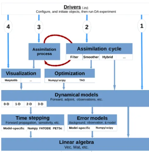
The design of DATeS takes into account the distinction be-tween these components and separates them in design fol-lowing an object-oriented programming (OOP) approach. A general description of DATeS architecture is given in Fig. 1.
The enumeration in Fig. 1 (numbers from 1 to 4 in cir-cles) indicates the order in which essential DATeS objects should be created. Specifically, one starts with an instance of a model. Once a model object is created, an assimilation ob-ject is instantiated, and the model obob-ject is passed to it. An as-similation process object is then instantiated, with a reference to the assimilation object passed to it. The assimilation pro-cess object iterates the consecutive assimilation cycles and saves and/or outputs the results which can be optionally ana-lyzed later using visualization modules.
pack-Figure 1.Diagram of the DATeS architecture.
age. DATeS provides base classes with definitions of the nec-essary methods. A new class added to DATeS, for example, to implement a specific new model, has to inherit the appro-priate model base class and provide implementations of the inherited methods from that base class.
In order to maximize both flexibility and generalizabil-ity, we opted to handle configurations, inputs, and output of DATeS object using “configuration dictionaries”. Parameters passed to instantiate an object are passed to the class con-structor in the form of key-value pairs in the dictionaries. See Sect. 4 for examples on how to properly configure and instantiate DATeS objects.
3.2 Linear algebra classes
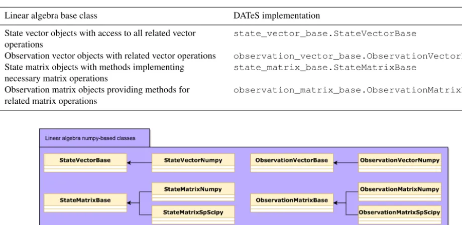
The main linear algebra data structures essential for almost all DA aspects are (a) model state-size and observation-size vectors (also named state and observation vectors, respec-tively), and (b) state-size and observation-size matrices (also named state and observation matrices, respectively). A state matrix is a square matrix of order equal to the model state-space dimension. Similarly, an observation matrix is a square matrix of order equal to the model observation space dimen-sion. DATeS makes a distinction between state and obser-vation linear algebra data structures. It is important to re-call here that, in large-scale applications, full state covari-ance matrices cannot be explicitly constructed in memory. Full state matrices should only be considered for relatively small problems and for experimental purposes. In large-scale settings, where building state matrices is infeasible, low-rank approximations or sparse representation of the
covari-ance matrices could be incorporated. DATeS provides simple classes to construct sparse state and observation matrices for guidance.
Third-party linear algebra routines can have widely differ-ent interfaces and underlying data structures. For reusability, DATeS provides unified interfaces for accessing and manip-ulating these data structures using Python classes. The linear algebra classes are implemented in Python. The functionali-ties of the associated methods can be written either in Python or in lower-level languages using proper wrappers. A class for a linear algebra data structure enables updating, slicing, and manipulating an instance of the corresponding data struc-tures. For example, a model state vector class provides meth-ods that enable accessing/slicing and updating entries of the state vector, a method for adding two state vector instances, and methods for applying specific scalar operations on all entries of the state vector such as evaluating the square root or the logarithm. Once an instance of a linear algebra data structure is created, all its associated methods are accessible via the standard Python dot operator. The linear algebra base classes provided in DATeS are summarized in Table 1.
Python special methods are provided in a linear al-gebra class to enable iterating a linear alal-gebra data structure entries. Examples of these special meth-ods include__getitem__( ), __setitem__( ), __getslice__( ), __setslice__( ), etc. These operators make it feasible to standardize working with linear algebra data structures implemented in different languages or saved in memory in different forms.
DATeS provides linear algebra data structures represented as NumPy ndarrays, and a set of NumPy-based classes to manipulate them. Moreover, SciPy-based implementation of sparse matrices is provided and can be used efficiently in conjunction with both sparse and non-sparse data structures. These classes, shown in Fig. 2, provide templates for de-signing more sophisticated extensions of the linear algebra classes.
3.3 Forecast model classes
Table 1.DA filtering routines provided by the initial version of DATeS (v1.0).
Linear algebra base class DATeS implementation
State vector objects with access to all related vector operations
state_vector_base.StateVectorBase
Observation vector objects with related vector operations observation_vector_base.ObservationVectorBase
State matrix objects with methods implementing necessary matrix operations
state_matrix_base.StateMatrixBase
Observation matrix objects providing methods for related matrix operations
observation_matrix_base.ObservationMatrixBase
Figure 2.Python implementation of state vector, observation vector, state matrix, and observation matrix data structures. Both dense and sparse state and observation matrices are provided.
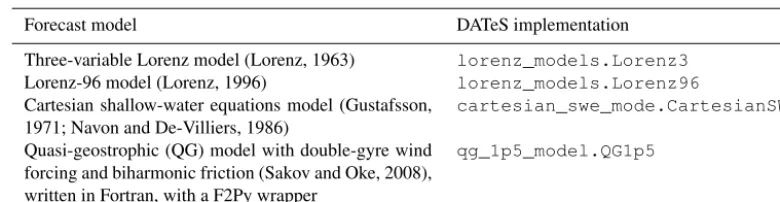
numerical model class. The package DATeS v1.0 includes implementations of several popular test models summarized in Table 2.
While some linear algebra and the time integration rou-tines are model-specific, DATeS also implements general-purpose linear algebra classes and time integration routines that can be reused by newly created models. For example, the general integration class FatODE_ERK_FWD is based on FATODE (Zhang and Sandu, 2014) explicit Runge–Kutta (ERK) forward propagation schemes.
3.4 Error model classes
In many DA applications, the errors are additive and are modeled by random variables normally distributed with zero mean and a given or an unknown covariance matrix. DATeS implements NumPy-based functionality for background, ob-servation, and model errors as guidelines for more sophisti-cated problem-dependent error models. The NumPy-based error models in DATeS are implemented in the module error_models_numpy. These classes are derived from the base classErrorsModelBaseand provide methodolo-gies to sample the underlying probability distribution, evalu-ate the value of the density function, and generevalu-ate statistics of the error variables based on model trajectories and the set-tings of the error model. Note that, while DATeS provides implementations for Gaussian error models, the Gaussian as-sumption itself is not restrictive. Following the same struc-ture, or by inheritance, one can easily create non-Gaussian error models with minimal efforts. Moreover, the Gaussian
error models provided by DATeS support both correlated and uncorrelated errors, and it constructs the covariance matri-ces accordingly. The covariance matrimatri-ces are stored in ap-propriate sparse formats, unless a dense matrix is explicitly requested. Since these covariance matrices are either state or observation matrices, they provide access to all proper linear algebra routines. This means that the code written with ac-cess to an observation error model and its components should work for both correlated and uncorrelated observations.
3.5 Assimilation classes
Assimilation classes are responsible for carrying out a sin-gle assimilation cycle (i.e., over one assimilation window) and optionally printing or writing the results to files. For example, an EnKF object should be designed to carry out one cycle consisting of the “forecast” and the “analysis” steps. The basic assimilation objects in DATeS are a filter-ing object, a smoothfilter-ing object, and a hybrid object. DATeS provides the common functionalities for filtering objects in the base class filters_base.FiltersBase; all de-rived filtering classes should have it as a super class. Simi-larly, smoothing objects are to be derived from the base class smoothers_base.SmoothersBase. A hybrid object can inherit methods from both filtering and smoothing base classes.
Table 2.DA filtering routines provided by the initial version of DATeS (v1.0).
Forecast model DATeS implementation
Three-variable Lorenz model (Lorenz, 1963) lorenz_models.Lorenz3
Lorenz-96 model (Lorenz, 1996) lorenz_models.Lorenz96
Cartesian shallow-water equations model (Gustafsson, 1971; Navon and De-Villiers, 1986)
cartesian_swe_mode.CartesianSWE
Quasi-geostrophic (QG) model with double-gyre wind forcing and biharmonic friction (Sakov and Oke, 2008), written in Fortran, with a F2Py wrapper
qg_1p5_model.QG1p5
Table 3.DA filtering routines provided by the initial version of DATeS v1.0.
Filtering algorithm DATeS implementation
Standard Kalman filter equations (Kalman and Bucy, 1961; Kalman, 1960) KF.KalmanFilter
Perturbed-observation (stochastic) EnKF (Burgers et al., 1998; EnKF.EnKF
Houtekamer and Mitchell, 1998)
Deterministic EnKF (Sakov and Oke, 2008) EnKF.DEnKF
Ensemble transform Kalman filter (ETKF) (Bishop et al., 2001) EnKF.ETKF
Local least-squares EnKF (Anderson, 2003) EnKF.LLSEnKF
Hybrid Monte Carlo (HMC) sampling filter (Attia and Sandu, 2015) hmc_filter.HMCFilter
Family of cluster sampling filters (Attia et al., 2018) multi_chain_mcmc_filter.MultiChainMCMC
A vanilla implementation of the particle filter (Gordon et al., 1993) PF.PF
the observation time, the assimilation time, the observation vector, and the forecast state or ensemble, are also passed to the constructor upon instantiation and can be updated during runtime.
Table 3 summarizes the filters implemented in the initial version of the package, which is DATeS v1.0. Each of these filtering classes can be instantiated and run with any of the DATeS model objects. Moreover, DATeS provides simpli-fied implementations of both 3D-Var and 4D-Var assimila-tion schemes. The objective funcassimila-tion, e.g., the negative log posterior, and the associated gradient are implemented in-side the smoother class and require the tangent linear model to be implemented in the passed forecast model class. The adjoint is evaluated using FATODE following a checkpoint-ing approach, and the optimization step is carried out uscheckpoint-ing SciPy optimization functions. The settings of the optimizer can be fine-tuned via the configuration dictionaries. The 3D-and 4D-Var implementations provided by DATeS are exper-imental and are provided as a proof of concept. The varia-tional aspects of DATeS are being continuously developed and will be made available in future releases of the package. Covariance inflation and localization are ubiquitously used in all ensemble-based assimilation systems. These two meth-ods are used to counteract the effect of using ensembles of finite size. Specifically, covariance inflation counteracts the loss of variance incurred in the analysis step and works by inflating the ensemble members around their mean. This is carried out by magnifying the spread of ensemble members around their mean by a predefined inflation factor. The
infla-tion factor could be a scalar, i.e., space–time independent, or even varied over space and/or time. Localization, on the other hand, mitigates the accumulation of long-range spurious cor-relations. Distance-based covariance localization is widely used in geoscientific sciences, and applications, where cor-relations are damped out with increasing distance between grid points. The performance of the assimilation algorithm is critically dependent on tuning the parameters of these tech-niques. DATeS provide basic utility functions (see Sect. 3.7) for carrying out inflation and localization which can be used in different forms based on the specific implementation of the assimilation algorithms. The work in Attia and Constan-tinescu (2018) reviews inflation and localization and presents a framework for adaptive tuning of the parameters of these techniques, with all implementations and numerical experi-ments carried out entirely in DATeS.
3.6 Assimilation process classes
Figure 3.The assimilation process in DATeS.
be found in Attia et al. (2018) and Attia and Constantinescu (2018), and in Sect. 4.6.
assimilation_process_base.Assimilation Processis the base class from which all assimilation pro-cess objects are derived. When instantiating an assimilation process object, the assimilation object, the observations, and the assimilation time instances are passed to the constructor through configuration dictionaries. As a result, the assimila-tion process object has access to the model and its associated data structures and functionalities through the assimilation object.
The assimilation process object either retrieves real obser-vations or creates synthetic obserobser-vations at the specified time instances of the experiment. Figure 3 summarizes DATeS as-similation process functionality.
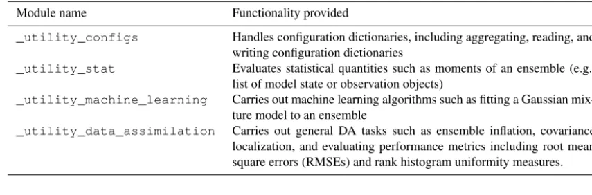
3.7 Utility modules
Utility modules provide additional functionality, such as the _utility_configs module which provides functions for reading, writing, validating, and aggregating configura-tion dicconfigura-tionaries. In DA, an ensemble is a collecconfigura-tion of state or observation vectors. Ensembles are represented in DATeS as lists of either state or observation vector objects. The util-ity modules include functions responsible for iterating over ensembles to evaluate ensemble-related quantities of inter-est, such as ensemble mean, ensemble variance/covariance, and covariance trace. Covariance inflation and localization are critically important for nearly all ensemble-based assim-ilation algorithms. DATeS abstracts tools and functions com-mon to assimilation methods, such as inflation and local-ization, where they can be easily imported and reused by newly developed assimilation routines. The utility module in DATeS provides methods to carry out these procedures in various modes, including state-space and observation space localization. Moreover, DATeS supports space-dependent
co-variance localization; i.e., it allows varying the localization radii and inflation factors over both space and time.
Ensemble-based assimilation algorithms often require ma-trix representation of ensembles of model states. In DATeS, ensembles are represented as lists of states, rather than full matrices of size Nstate×Nens. However, it provides utility functions capable of efficiently calculating ensemble statis-tics, including ensemble variances, and covariance trace. Moreover, DATeS provides matrix-free implementations of the operations that require ensembles of states, such as a matrix–vector product, where the matrix is involved in a rep-resentation of an ensemble of states.
The moduledates_utilityprovides access to all util-ity functions in DATeS. In fact, this module wraps the func-tionality provided by several other specialized utility rou-tines, including the sample given in Table 4. The utility mod-ule provides other general functions such as handling file downloading, and functions for file I/O. For a list of all func-tions in the utility module, see the user manual (Attia et al., 2016).
4 Using DATeS
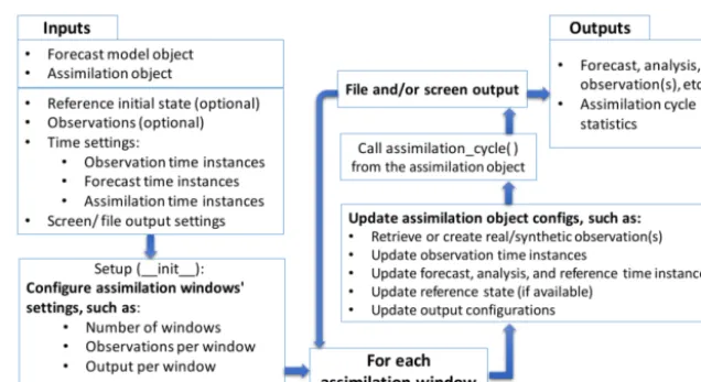
The sequence of steps needed to run a DA experiment in DATeS is summarized in Fig. 4. This section is devoted to explaining these steps in the context of a working example that uses the QG-1.5 model (Sakov and Oke, 2008) and car-ries out DA using a standard EnKF formulation.
4.1 Step1: initialize DATeS
Table 4.A sample of the modules wrapped by the main utility moduledates_utility.
Module name Functionality provided
_utility_configs Handles configuration dictionaries, including aggregating, reading, and writing configuration dictionaries
_utility_stat Evaluates statistical quantities such as moments of an ensemble (e.g., list of model state or observation objects)
_utility_machine_learning Carries out machine learning algorithms such as fitting a Gaussian mix-ture model to an ensemble
_utility_data_assimilation Carries out general DA tasks such as ensemble inflation, covariance localization, and evaluating performance metrics including root mean square errors (RMSEs) and rank histogram uniformity measures.
Figure 4.The sequence of essential steps required in order to run a DA experiment in DATeS.
Figure 5.Initializing the DATeS run.
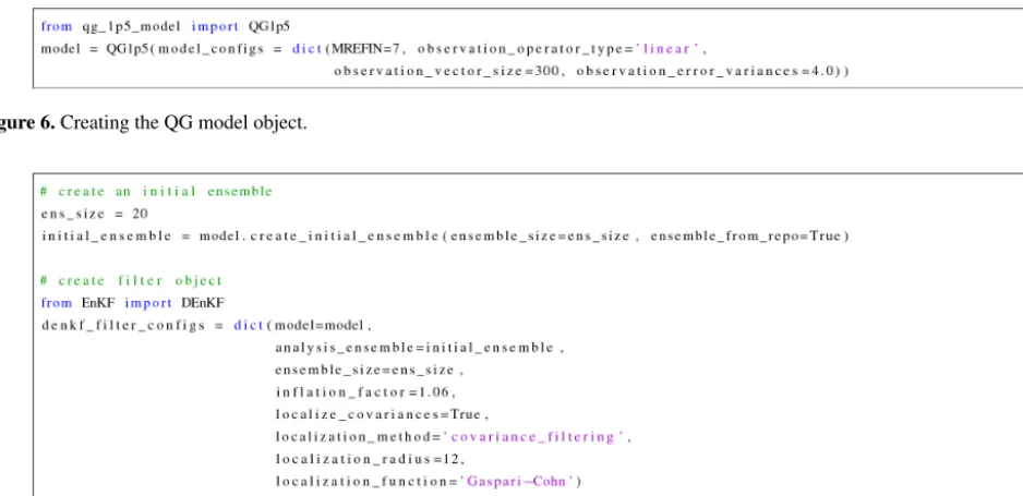
4.2 Step2: create a model object
QG-1.5 is a nonlinear 1.5-layer reduced-gravity QG model with double-gyre wind forcing and biharmonic friction (Sakov and Oke, 2008).
4.2.1 Quasi-geostrophic model
This model is a numerical approximation of the equations qt=ψx−εJ (ψ, q)−A13ψ+2πsin(2πy),
q=1ψ−F ψ,
J (ψ, q)≡ψxqx−ψyqy, (9) where 1:=∂2/∂x2+∂2/∂y2 and ψ is the surface eleva-tion. The values of the model coefficients in Eq. (9) are ob-tained from Sakov and Oke (2008) and are described as fol-lows:F =1600,ε=10−5, andA=2×10⁻¹². The domain of the model is a 1×1 (space units) square, with 0≤x≤1, 0≤y≤1, and is discretized by a grid of size 129×129 (including boundaries). The boundary conditions used are ψ=1ψ=12ψ=0. The dimension of the model state vec-tor is Nstate=16 641. This is a synthetic model where the scales are not relevant, and we use generic space, time, and solution amplitude units. The time integration scheme used is the fourth-order Runge–Kutta scheme with a time step of 1.25 (time units). The model forward propagation core is implemented in Fortran. The QG-1.5 model is run over 1000 model time steps, with observations made available ev-ery 10 time steps.
4.2.2 Observations and observation operators
We use a standard linear operator to observe 300 compo-nents ofψ with observation error variance set to 4.0 (units squared). The observed components are uniformly dis-tributed over the state vector length, with an offset that is randomized at each filtering cycle. Synthetic observations are obtained by adding white noise to measurements of the sea surface height level (SSH) extracted from a reference model run with lower viscosity. To create a QG model object with these specifications, one executes the code snippet in Fig. 6.
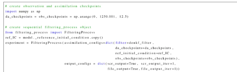
4.3 Step3: create an assimilation object
One now proceeds to create an assimilation object. We con-sider a deterministic implementation of EnKF (DEnKF) with ensemble size equal to 20, and parameters tuned optimally as suggested in Sakov and Oke (2008). Covariance local-ization is applied via a Hadamard product (Houtekamer and Mitchell, 2001). The localization function is Gaspari–Cohn (Gaspari and Cohn, 1999) with a localization radius of 12 grid cells. The localization is carried out in the observation space by decorrelating bothHBandHBHT, whereBis the ensemble covariance matrix, andHis the linearized observa-tion operator. In the present setup, the observaobserva-tion operator His linear, and thusH=H.
Figure 6.Creating the QG model object.
Figure 7.Creating a DEnKF filtering object.
with an inflation factor of 1.06. The code snippet in Fig. 7 creates a DEnKF filtering object with these settings.
Most of the methods associated with the DEnKF object will raise exceptions if immediately invoked at this point. This is because several keys in the filter configuration dictio-nary, such as the observation, the forecast time, the analysis time, and the assimilation time, are not yet appropriately as-signed. DATeS allows creating assimilation objects without these options to maximize flexibility. A convenient approach is to create an assimilation process object that, among other tasks, can properly update the filter configurations between consecutive assimilation cycles.
4.4 Step4: create an assimilation process
We now test DEnKF with the QG model by repeating the as-similation cycle over a time span from 0 to 1250 with offsets of 12.5 time units between each two consecutive observa-tion/assimilation times. An initial ensemble is created by the numerical model object. An experimental time span is set for observations and assimilation. Here, the assimilation time in-stancesda_checkpointsare the same as the observation time instancesobs_checkpoints, but they can in general be different, leading to either synchronous or asynchronous assimilation settings. This is implemented in the code snippet in Fig. 8.
Here, experiment is responsible for creating syn-thetic observations at all time instances defined by obs_checkpoints (except the initial time). To create synthetic observations, the truth at the initial time (0 in this case) is obtained from the model and is passed to the
filter-ing process objectexperiment, which in turn propagates it forward in time to assimilation time points.
Finally, the assimilation experiment is executed by run-ning the code snippet in Fig. 9.
4.5 Experiment results
The filtering results are printed to screen and are saved to files at the end of each assimilation cycle as instructed by the output_configs dictionary of the object experiment. The output directory structure is controlled via the options in the output configuration dictionary output_configsof theFilteringProcess object, i.e., experiment. All results are saved in appropriate subdirectories under a main folder named Results in the root directory of DATeS. We will refer to this directory henceforth as DATeS results directory. The default behavior of a FilteringProcess object is to create a folder named Filtering_Results in the DATeS results directory and to instruct the filter object to save/output the results every file_output_iter whenever the flag file_outputis turned on. Specifically, theDEnKFobject creates three directories named Filter_Statistics,
Model_States_Repository, and
Figure 8.Creating a filter process object to carry out DEnKF filtering using the QG model.
Figure 9.Running the filtering experiment.
to False. The true solution (reference state), the anal-ysis ensemble, and the forecast ensembles are all saved under the directory Model_States_Repository, while the observations are saved under the directory Observations_Repository. We note that, while here we illustrate the default behavior, the output directories are fully configurable.
Figure 10 shows the reference initial state of the QG model, an example of the observational grid used, and an ini-tial forecast state. The iniini-tial forecast state in Fig. 10 is the average of an initial ensemble collected from a long run of the QG model.
The true field, the forecast errors, and the DEnKF analyses errors at different time instances are shown in Fig. 11.
Typical solution quality metrics in the ensemble-based DA literature include RMSE plots and rank (Talagrand) his-tograms (Anderson, 1996; Candille and Talagrand, 2005).
Upon termination of a DATeS run, executable files can be cleaned up by calling the function clean_executable_files( ) available in the utility module (see the code snippet in Fig. 12).
4.6 DATeS for benchmarking 4.6.1 Performance metrics
In the linear settings, the performance of an ensemble-based DA filter could be judged based on two factors. Firstly, con-vergence is explained by its ability to track the truth and sec-ondly by the quality of the flow-dependent covariance matrix generated given the analysis ensemble.
The convergence of the filter is monitored by inspecting the RMSE, which represents an ensemble-based standard de-viation of the difference between reality, or truth, and the model-based prediction. In synthetic experiments, where the
Figure 10.The QG-1.5 model. The truth (reference state) at the initial time (t=0) of the assimilation experiment is shown in panel(a). The red dots indicate the locations of observations for one of the test cases employed. The initial forecast state, taken as the av-erage of the initial ensemble at timet=0, is shown in panel(b).
Figure 11.Data assimilation results. The reference fieldψ, the fore-cast errors, and the analysis errors att=300,t=600,t=900, and
Figure 12.Cleanup of DATeS executable files.
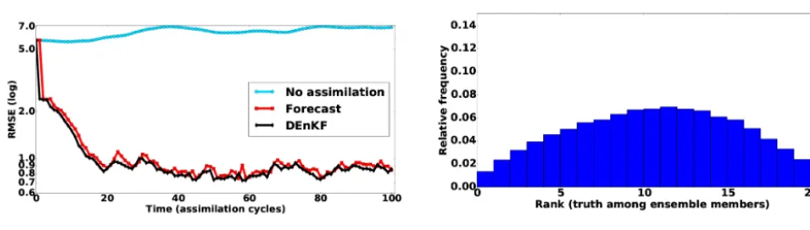
Figure 13.Data assimilation results. In panel(a), “no assimilation” refers to the RMSE of the initial forecast (the average of the initial forecast ensemble) propagated forward in time over the 100 cycles without assimilating observations into it. The rank histogram of where the truth ranks among analysis ensemble members is shown in panel(b). The ranks are evaluated for every 13th variable in the state vector (past the correlation bound) after 100 assimilation cycles.
model representation of the truth is known, the RMSE reads
RMSE= v u u t
1 Nstate
Nstate X
i=1
(xi−xiTrue)
2, (10)
where x=(x1, x2, . . ., xNstate)
T ∈
RNstate is the prediction at a given time instant, e.g., the forecast ensemble mean, and xTrue∈RNstate is the verification, e.g., the true model state
at the same time instant. For real applications, the states are generally replaced with observations. The rank (Talagrand) histogram (Anderson, 1996; Candille and Talagrand, 2005) could be used to assess the spread of the ensemble and its coverage to the truth. Generally speaking, the rank histogram plots the rank of the truth (or observations) compared to the ensemble members (or equivalent observations), ordered in-creasingly in magnitude. A nearly uniform rank histogram is desirable and suggests that the truth is indistinguishable from the ensemble members. A mound rank histogram indicates an overdispersed ensemble, a while U-shaped histogram in-dicates underdispersion. However, mound rank histograms are rarely seen in practice, especially for large-scale prob-lems. See, e.g., Hamill (2001) for a mathematical description and a detailed discussion on the usefulness and interpretation of rank histograms.
Figure 13a shows an RMSE plot of the results of the ex-periment presented in Sect. 4.5. The histogram of the rank statistics of the truth, compared to the analysis ensemble, is shown in Fig. 13b.
For benchmarking, one needs to generate scalar represen-tations of the RMSE and the uniformity of a rank histogram of a numerical experiment. The average RMSE can be used
to compare the accuracy of a group of filters. To generate a scalar representation of the uniformity of a rank histogram, we fit a beta distribution to the rank histogram, scaled to the interval[0,1], and evaluate the Kullback–Leibler (KL) divergence (Kullback and Leibler, 1951) between the fit-ted distribution and a uniform distribution. The KL di-vergence between two beta distributions Beta(α, β), and Beta(α0, β0)isDKL Beta(α, β)|Beta(α0β0)
=ln0(α+β)− ln(α β)−ln0(α0+β0)+ln(α0β0)+(α−α0) ψ (α)−ψ (α0)+ (β−β0) ψ (β)−ψ (β0), where ψ (·)=00(·)/ 0(·) is the digamma function, i.e., the logarithmic derivative of the gamma function. Here, we set Beta(α0, β0)to a uniform dis-tribution by settingα0=β0=1. We consider a small, e.g., closer to 0, KL distance to be an indication of a nearly uni-form rank histogram and consequently an indication of a well-dispersed ensemble. An alternative measure of rank his-togram uniformity is to average the absolute distances of bins’ heights from a uniformly distributed rank histogram (Bessac et al., 2018). DATeS provides several utility func-tions to calculate such metrics for a numerical experiment.
distribu-Figure 14.Rank histograms with fitted beta distributions. The KL-divergence measure is indicated under each panel.
Table 5.Measures of uniformity of the rank histograms shown in Fig. 14.
Panel 1 2 3 4 5 6
DKL(β|U) 0.198 0.231 0.022 0.018 0.065 0.272
Average distance toU 0.085 0.038 0.005 0.011 0.008 0.010
tion with respect to a uniform one, and the average distances between histogram bins and a uniform one.
4.6.2 Benchmarking
The architecture of DATeS makes it easy to generate bench-marks for a new experiment. For example, one can write short scripts to iterate over a combination of settings of a fil-ter to find the best possible results. As an example, consider the standard 40-variable Lorenz-96 model (Lorenz, 1996) de-scribed by the equations
dxi
dt =xi−1(xi+1−xi−2)−xi+F; i=1,2, . . .,40, (11) where x=(x1, x2, . . ., x40)T ∈R40 is the state vector, with periodic boundaries, i.e., x0≡x40, and the forcing param-eter is set toF =8. These settings make the system chaotic (Lorenz and Emanuel, 1998) and are widely used in synthetic settings for geoscientific applications. Adjusting the inflation factor and the localization radius for EnKF filter is crucial. Consider the case where one is testing an adaptive inflation scheme and would like to decide on the ensemble size and the benchmark inflation factor to be used. As an example of benchmarking, we run the following experiment over a time interval[0,30](units), where Eq. (11) is integrated for-ward in time using a fourth-order Runge–Kutta scheme with model step size 0.005 (units). Assume that synthetic observa-tions are generated every 20 model steps, where every other entry of the model state is observed. We test the DEnKF
al-gorithm, with the fifth-order piecewise-rational function of Gaspari and Cohn (Gaspari and Cohn, 1999) for covariance localization. The localization radius is held constant and is set tol=4, while the inflation factor is varied for each ex-periment. The experiments are repeated for ensemble sizes Nens=5,10, . . .,40. We report the results over the last two-thirds of the experiments’ time span, i.e., over the interval [10,30], to avoid spinup artifacts. This interval, consisting of the last 200 assimilation cycles out of 300, will be referred to as the “testing time span”. Any experiment that results in an average RMSE of more than 0.65 over the testing time span is discarded, and the filter used is seen to diverge. The numerical results are summarized in Figs. 15 and 16.
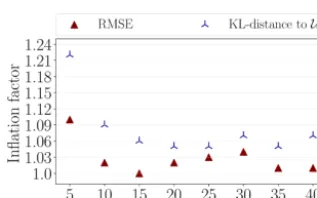
Figure 15 shows the average RMSE results and the KL distances between a beta distribution fitted to the analysis rank histogram of each experiment, and a uniform distri-bution. These plots give a preliminary idea of the plausible regimes of both ensemble size and inflation factor that should be used to achieve the best performance of the filter used under the current experimental settings. For example, for an ensemble sizeNens=20, the inflation factor should be set approximately to 1.01–1.07 to give both a small RMSE and an analysis rank histogram close to uniform.
ex-Figure 15.Data assimilation results with DEnKF applied to Lorenz-96 system. RMSE results on a log scale are shown in panel(a). The KL distances between the analysis rank histogram and a uniform rank histogram are shown in panel(b). The localization radius is fixed to 4.
Figure 16. Data assimilation results with DEnKF applied to Lorenz-96 system. The minimum average RMSE over the inter-val[10,30]is indicated by red triangles. The minimum average KL distance between the analysis rank histogram and a uniformly dis-tributed rank histogram[10,30] is indicated by blue tripods. We show the results for every choice of the ensemble size. The local-ization radius is fixed to 4.
periment that resulted in minimum average RMSE over the testing time span, out of all benchmarking experiments car-ried out with this ensemble size. Similarly, the experiment that yielded minimum KL divergence to a uniform rank his-togram is indicated by a blue tripod.
To answer the question about the ensemble size, we pick the ensemble sizeNens=25, given the current experimental setup. The reason is thatNens=25 is the smallest ensemble size that yields small RMSE and is a well-dispersed ensem-ble as explained by Fig. 16. As for the benchmark inflation factor, the results in Fig. 16 show that for an ensemble size Nens=25, the best choice of an inflation factor is approxi-mately 1.03–1.05 for Gaspari–Cohn localization with a fixed radius of 4.
Despite being a relatively easy process, unfortunately, gen-erating a set of benchmarks for all possible combinations of numerical experiments is a time-consuming process and is better carried out by the DA community. Some example scripts for generating and plotting benchmarking results are included in the package for guidance.
Note that, when the Gaussian assumption is severely vio-lated, standard benchmarking tools, such as RMSE and rank
histograms, should be replaced with, or at least supported by, tools capable of assessing ensemble coverage of the poste-rior distribution. In such cases, MCMC methods, including those implemented in DATeS (Attia and Sandu, 2015; Attia et al., 2018; Attia, 2016), could be used as a benchmarking tool (Law and Stuart, 2012).
5 Extending DATeS
DATeS aims at being a collaborative environment and is de-signed such that adding DA components to the package is as easy and flexible as possible. This section describes how new implementations of components such as numerical mod-els and assimilation methodologies can be added to DATeS.
The most direct approach is to write the new implementa-tion completely in Python. This, however, may sacrifice ef-ficiency or may not be feasible when existing code in other languages needs to be reused. One of the main characteristics of DATeS is the possibility of incorporating code written in low-level languages. There are several strategies that can be followed to interface existing C or Fortran code with DATeS. Amongst the most popular tools are SWIG and F2Py for in-terfacing Python code with existing implementations written in C and Fortran, respectively.
Whether the new contribution is written in Python, in C, or in Fortran, an appropriate Python class that inherits the corre-sponding base class, or a class derived from it, has to be cre-ated. The goal is to design new classes that are conformable with the existing structure of DATeS and can interact appro-priately with new as well as existing components.
5.1 Adding a numerical model class
Figure 17.Illustration of a numerical model class namedMyModeland relations to the linear algebra and error models classes. A dashed arrow refers to an “import” relation, and a solid arrow represents an “inherit” relation.
The first step is to grant the model object access to lin-ear algebra data structures and to error models. Appropriate classes should be imported in a numerical model class:
– Linear algebra includes state vector, state matrix, obser-vation vector, and obserobser-vation matrix.
– Error models include background, model, and observa-tion error models.
This gives the model object access to model-based data structures and error entities necessary for DA applications. Figure 17 illustrates a class of a numerical model named MyModel, along with all the essential classes imported by it.
The next step is to create Python-based implementations for the model functionalities. As shown in Fig. 17, the corre-sponding methods have descriptive names in order to ease the use of DATeS functionality. For example, the method state_vector( ) creates (or initializes) a state vector data structure. Details of each of the methods in Fig. 17 are given in the DATeS user manual (Attia et al., 2016).
As an example, suppose we want to create a model class name MyModel using NumPy and SciPy (for sparse ma-trices) linear algebra data structures. The code snippet in Fig. 18 shows the implementation of such a class.
Figure 18.The leading lines of an implementation of a class for the modelMyModelderived from the models’ base classModelsBase. Linear algebra objects are derived from NumPy-based (or SciPy-based) objects.
with linear algebra classes, and even if only binary files are provided, the Python-based linear algebra methods must be implemented. If the model functionality is fully written in Python, the implementation of the methods associated with a model class is straightforward, as illustrated in Attia et al. (2016). On the other hand, if a low-level implementation of a numerical model is given, these methods wrap the corre-sponding low-level implementation.
5.2 Adding an assimilation class
The process of adding a new class for an assimilation methodology is similar to creating a class for a numerical model; however, it is expected to require less effort. For ex-ample, a class implementation of a filtering algorithm uses components and tools provided by the passed model and by the encapsulated linear algebra data structures and methods. Moreover, filtering algorithms belonging to the same fam-ily, such as different flavors of the well-known EnKF, are expected to share a considerable amount of infrastructure. Python inheritance enables the reuse of methods and vari-ables from parent classes.
To create a new class for DA filtering, one derives it from the base classFiltersBase, imports appropriate routines, and defines the necessary functionalities. Note that each as-similation object has access to a model object and
conse-quently to the proper linear algebra data structures and as-sociated functionalities through that model.
Unlike the base class for numerical models (ModelsBase), the filtering base class FiltersBase includes actual implementations of several widely used solvers. For example, an implementation of the method FiltersBase.filtering_cycle( ) is provided to carry out a single filtering cycle by applying a forecast phase followed by an analysis phase (or vice versa, depending on stated configurations).
Figure 19 illustrates a filtering class namedMyFilter that works by carrying out analysis and forecast steps in the ensemble-based statistical framework.
The code snippet in Fig. 20 shows the leading lines of an implementation of theMyFilterclass.
6 Discussion and concluding remarks
Figure 19.Illustration of a DA filtering classMyFilterand its relation to the filtering base class. A solid arrow represents an “inherit” relation.
Figure 20.The leading lines of an implementation of a DA filter; theMyFilterclass is derived from the filters’ base classFiltersBase.
languages such as C or Fortran to attain high levels of com-putational efficiency.
While we introduced several assimilation schemes in this paper, the current version, DATeS v1.0, emphasizes the sta-tistical assimilation methods. DATeS provide the essential infrastructure required to combine elements of a variational assimilation algorithm with other parts of the package. The variational aspects of DATeS, however, require additional work that includes efficient evaluation of the adjoint model,
checkpointing, and handling weak constraints. A new version of the package, under development, will carefully address these issues and will provide implementations of several vari-ational schemes. The varivari-ational implementations will be de-rived from the 3D- and 4D-Var classes implemented in the current version (DATeS v1.0).
research-grade implementations. DATeS is well suited for educational purposes as a learning tool for students and newcomers to the data assimilation research field. It can also help data assim-ilation researchers develop specific components of the data assimilation process and easily use them with the existing elements of the package. For example, one can develop a new filter and interface an existing physical model, and error models, without the need to understand how these compo-nents are implemented. This requires unifying the interfaces between the different components of the data assimilation process, which is an essential feature of DATeS. These fea-tures allow for optimal collaboration between teams working on different aspects of a data assimilation system.
To contribute to DATeS, by adding new implementations, one must comply with the naming conventions given in the base classes. This requires building proper Python interfaces for the implementations intended to be incorporated with the package. Interfacing operational models, such the Weather Research and Forecasting (WRF) model (Skamarock et al., 2005), in the current version, DATeS v1.0, is expected to re-quire substantial work. Moreover, DATeS does not yet sup-port parallelization, which limits its applicability in opera-tional settings.
The authors plan to continue developing DATeS with the long-term goal of making it a complete data assimila-tion testing suite that includes support for variaassimila-tional meth-ods, as well as interfaces with complex models such as quasi-geostrophic global circulation models. Parallelization of DATeS, and interfacing large-scale models such as the WRF model, will also be considered in the future.
Code and data availability. The code of DATeS v1.0 is available at https://doi.org/10.5281/zenodo.1323207 (Attia, 2018). The on-line documentation and alternative download links are available at http://people.cs.vt.edu/~attia/DATeS/index.html (last access:2 Jan-uary 2019).
Author contributions. AA developed the package and performed the numerical simulations. The two authors wrote the paper, and AS supervised the whole project.
Competing interests. The authors declare that they have no conflict of interest.
Acknowledgements. The authors would like to thank Ma-hesh Narayanamurthi, Paul Tranquilli, Ross Glandon, and Arash Sarshar from the Computational Science Laboratory (CSL) at Virginia Tech, and Vishwas Rao from the Argonne National Lab-oratory, for their contributions to an initial version of DATeS. This work has been supported in part by awards NSF CCF-1613905, NSF ACI–1709727, and AFOSR DDDAS 15RT1037, and by the CSL at Virginia Tech.
Edited by: Ignacio Pisso
Reviewed by: Kody Law and three anonymous referees
References
Ades, M. and van Leeuwen, P. J.: The equivalent-weights particle filter in a high-dimensional system, Q. J. Roy. Meteor. Soc., 141, 484–503, 2015.
Anderson, J. L.: A method for producing and evaluating probabilis-tic forecasts from ensemble model integrations, J. Climate, 9, 1518–1530, 1996.
Anderson, J. L.: A local least squares framework for ensemble fil-tering, Mon. Weather Rev., 131, 634–642, 2003.
Anderson, J. L., Hoar, T., Raeder, K., Liu, H., Collins, N., Torn, R., and Avellano, A.: The data assimilation research testbed: A com-munity facility, B. Am. Meteorol. Soc., 90, 1283–1296, 2009. Asch, M., Bocquet, M., and Nodet, M.: Data assimilation: methods,
algorithms, and applications, The Society for Industrial and Ap-plied Mathematics (SIAM), Philadelphia, USA, vol. 11, ISBN 9781611974539, 2016.
Attia, A.: Advanced Sampling Methods for Solving Large-Scale Inverse Problems, PhD thesis, Virginia Tech, available at: http: //hdl.handle.net/10919/73683 (last access: 2 February 2019), 2016.
Attia, A.: a-attia/DATeS: Initial version of DATeS (Version v1.0), Zenodo, https://doi.org/10.5281/zenodo.1323207, 2018. Attia, A. and Constantinescu, E.: An Optimal Experimental Design
Framework for Adaptive Inflation and Covariance Localization for Ensemble Filters, arXiv preprint arXiv:1806.10655, under re-view, 2018.
Attia, A. and Sandu, A.: A Hybrid Monte Carlo sampling filter for non-Gaussian data assimilation, AIMS Geosciences, 1, 41–78, https://doi.org/10.3934/geosci.2015.1.41, 2015.
Attia, A., Rao, V., and Sandu, A.: A sampling approach for four di-mensional data assimilation, in: Dynamic Data-Driven Environ-mental Systems Science, Springer, Cham, Switzerland, 215–226, 2015.
Attia, A., Glandon, R., Tranquilli, P., Narayanamurthi, M., Sarshar, A., and Sandu, A.: DATeS: A Highly-Extensible Data Assim-ilation Testing Suite, available at: http://people.cs.vt.edu/~attia/ DATeS (last access: 2 January 2019), 2016.
Attia, A., Rao, V., and Sandu, A.: A Hybrid Monte Carlo sampling smoother for four dimensional data assimilation, Int. J. Numer. Meth. Fl., 83, 90–112, https://doi.org/10.1002/fld.4259, 2017a. Attia, A., Stefanescu, R., and Sandu, A.: The Reduced-Order
Hy-brid Monte Carlo Sampling Smoother, Int. J. Numer. Meth. Fl., 83, 28–51, https://doi.org/10.1002/fld.4255, 2017b.
Attia, A., Moosavi, A., and Sandu, A.: Cluster Sampling Fil-ters for Non-Gaussian Data Assimilation, Atmosphere, 9, 213, https://doi.org/10.3390/atmos9060213, 2018.
Beazley, D. M.: SWIG: An Easy to Use Tool for Integrating Script-ing Languages with C and C++, in: Proc. 4th USENIX Tcl/Tk Workshop, 10–13 July 1996 Monterey, California, USA, 129– 139, 1996.