www.geosci-model-dev.net/6/117/2013/ doi:10.5194/gmd-6-117-2013
© Author(s) 2013. CC Attribution 3.0 License.
Geoscientific
Model Development
Using multi-model averaging to improve the reliability of catchment
scale nitrogen predictions
J.-F. Exbrayat1,2, N. R. Viney3, H.-G. Frede2, and L. Breuer2
1Climate Change Research Centre, University of New South Wales, Sydney, New South Wales, Australia 2Institute for Landscape Ecology and Resources Management (ILR), Research Centre for BioSystems,
Land Use and Nutrition (IFZ), Justus-Liebig-Universit¨at Gießen, Germany
3CSIRO Land and Water, Canberra, ACT, Australia
Correspondence to: J.-F. Exbrayat ([email protected])
Received: 26 June 2012 – Published in Geosci. Model Dev. Discuss.: 20 August 2012 Revised: 18 December 2012 – Accepted: 2 January 2013 – Published: 29 January 2013
Abstract. Hydro-biogeochemical models are used to foresee the impact of mitigation measures on water quality. Usually, scenario-based studies rely on single model applications. This is done in spite of the widely acknowledged advantage of ensemble approaches to cope with structural model un-certainty issues. As an attempt to demonstrate the reliabil-ity of such multi-model efforts in the hydro-biogeochemical context, this methodological contribution proposes an adap-tation of the reliability ensemble averaging (REA) philoso-phy to nitrogen losses predictions. A total of 4 models are used to predict the total nitrogen (TN) losses from the well-monitored Ellen Brook catchment in Western Australia. Sim-ulations include re-predictions of current conditions and a set of straightforward management changes targeting fertilisa-tion scenarios. Results show that, in spite of good calibrafertilisa-tion metrics, one of the models provides a very different response to management changes. This behaviour leads the simple av-erage of the ensemble members to also predict reductions in TN export that are not in agreement with the other models. However, considering the convergence of model predictions in the more sophisticated REA approach assigns more weight to previously less well-calibrated models that are more in agreement with each other. This method also avoids having to disqualify any of the ensemble members.
1 Introduction
Nowadays, mathematical models are often used to assess the impact of changes in boundary conditions on a natural sys-tem. More precisely, in the hydro-biogeochemical context,
they are used to study the effect of changes in management practices (e.g. fertilisation rate), climate and land-use cover (e.g. clear-cutting, reforestation) on the water and nutrient balances (e.g. Arheimer et al., 2005; Breuer and Huisman, 2009; Zammit et al., 2005). Most of the time, the adopted methodology is to use a single model calibrated to match well with current conditions. Then, some modifications mimick-ing real world changes are imposed on the relevant boundary conditions resulting in a set of scenarios. The actual scenario prediction is produced by re-running the model with these updated drivers. Impacts can be estimated as the difference between the original model outcomes and the altered ones in either a relative or an absolute way. Optimally, these predic-tions should be compared to the actual post-change observa-tions to assess their reliability but, in the case of land-use or climate change, this is seldom done as such data are typically not available. Nevertheless, some major concerns arise from this straightforward methodology in catchment scale hydro-biogeochemical model predictions.
and simulations is acceptable, based on some goodness-of-fit criteria (e.g. Legates and McCabe Jr., 1999). Although a lot of effort has been put into developing ever more efficient op-timisation algorithms for the last two decades (Duan et al., 1992; Vrugt et al., 2003), the ability of these models to ade-quately simulate the impact of changed boundary conditions is of concern (Huisman et al., 2009), especially since predic-tions are almost never validated against post-change obser-vations (Whitehead et al., 2002).
Second, it is now widely acknowledged that several pa-rameter sets may perform equally well (Beven, 2006) and that the outcome of a successful calibration procedure may indeed not be the actual best result. Therefore, an option to address the uncertainty in predictions, especially in the case of scenario predictions, is to use ensembles of multi-model predictions gathering the information content of several sim-ulations. Single-model ensembles regroup predictions ob-tained with the same model structure whilst altering param-eter values and boundary conditions in a Monte-Carlo pro-cedure like the GLUE methodology for example (Beven and Freer, 2001). Nevertheless, part of the predictive uncertainty is also linked to sometimes huge differences between model structures developed to address the same issues. As stated by Breuer et al. (2008) this is especially true in the context of hydro-biogeochemical predictions. In order to cope with structural uncertainties, it has become state-of-the-art to con-sider more than one model of the same system. These ensem-bles of predictions have been used in the fields of climate, weather, flood forecasting, rainfall-runoff and sub-surface flow, and a first multi-model comparison approach targeting agricultural fluxes of nitrogen was published by Diekkr¨uger et al. (1995). But to our knowledge, the ensemble methodol-ogy has received little interest in the nutrient fluxes context to date, in spite of the demonstrated improvement in prediction reliability. Furthermore, the few available studies, including previous publications by our working group, have only been based on re-prediction (hindcasting) efforts rather than sce-nario analyses (Exbrayat et al., 2010, 2011; Kronvang et al., 2009). Therefore, we present here an example of the poten-tial advantage of using multi-model predictions to assess the impact of a simple management change on the nutrient bal-ance of a well-monitored mesoscale catchment in south-west Western Australia.
2 Experimental setup
2.1 The Ellen Brook catchment
The Ellen Brook catchment (570 km2) is located in coastal SW Western Australia and contributes significantly to the water (6 %) and N loads (10 %) entering the Swan–Canning estuary that drains the city of Perth (Viney and Sivapalan, 2001). Most of the catchment has been cleared for agricul-tural purposes (Swan River Trust, 2007).
Jan Feb Mar Apr May Jun Jul Aug Sep Oct Nov Dec 0
1 2 3 4 5
Av
er
ag
e c
on
ce
nt
ra
tio
n
[m
g
N
L
−
1] Total N
Organic N NO3-N
NH4-N
Flow
0 1 2 3 4
Av
er
ag
e d
ail
y r
un
of
f [
m
3s
−
1] NH4-N
NO3-N
Organic N
Fig. 1. Seasonal cycle and relative contribution of different species
to TN (pie chart) in the Ellen Brook (1989–2006). Missing values in March and April correspond to no flow periods.
Hydro-climatic conditions are typical of a Mediterranean influence with a mean annual rainfall ranging from 510 to 830 mm yr−1 (1989–2006), derived from inverse distance
weighted interpolation from the 4 Australian Bureau of Me-teorology rain gauges located in the catchment. Intra-annual precipitation is distributed in cool and wet winters and warm and dry summers corresponding to high flow (May–June to September–October) and low to no flow periods (October– November to April–May), respectively (Fig. 1). Pan evap-oration is high (∼2000 mm yr−1)and because of the sandy nature of the soils, runoff is mostly generated as a quick and peaky response to rainfall events which explains a five-fold difference between minimum and maximum annual dis-charge over the study period. Soil texture does not allow the adsorption of large quantities of dissolved organic matter (Petrone et al., 2009). Furthermore, dissolved organic nitro-gen that accumulates in the groundwater slowly discharges in high concentration into the surface water during the driest months (Donohue et al., 2001).
As shown in Fig. 1, about 10 % of the TN flowing out of the Ellen Brook catchment is in the form of dissolved inor-ganic N (NO3-N and NH4-N) derived from animal wastes
and fertilisers used for agriculture and private gardens (Swan River Trust, 2007). Dominant organic N forms are either present in dissolved forms of degrading matter or parti-cles composed of plant and animal debris. Concentrations of all N forms rise up during autumn and winter (May– September) because they are flushed with surface runoff. They fall in early spring (September–November) as rainfall, hence runoff, decreases in intensity (Fig. 1). Slight increases in concentrations in December (Fig. 1) may be attributed to either evapotranspiration induced concentration phenomena or animals entering the stream more frequently during these hot periods (Swan River Trust, 2007).
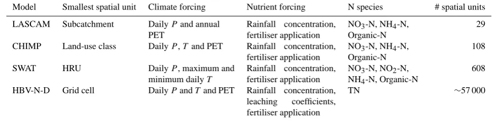
Table 1. Model characteristics.
Model Smallest spatial unit Climate forcing Nutrient forcing N species # spatial units
LASCAM Subcatchment DailyPand annual PET
Rainfall concentration, fertiliser application
NO3-N, NH4-N,
Organic-N
29
CHIMP Land-use class DailyP,T and PET Rainfall concentration, fertiliser application
NO3-N, NH4-N,
Organic-N
108
SWAT HRU DailyP, maximum and minimum dailyT
Rainfall concentration, fertiliser application
NO3-N, NO2-N,
NH4-N, Organic-N
608
HBV-N-D Grid cell DailyP andT and PET Rainfall concentration, leaching coefficients, fertiliser application
TN ∼57 000
P: precipitation, PET: potential evapotranspiration,T: air temperature, HRU: hydrological response unit.
and erosion, re-vegetation to stabilise river banks, increased community awareness to encourage reductions in fertiliser use, nutrient traps, improved monitoring of hot spots. Mean-while, a large monitoring effort has been undertaken and more than 900 daily samples of total nitrogen (TN) concen-trations are available at the Ellen Brook outlet out of a to-tal of 3870 days with runoff between 1989 and 2006. Over this period, mean TN concentration was 2.1 mg N L−1 with
values ranging from 0.3 to 7.4 mg N L−1with no significant
long-term temporal trend. This rich dataset allows a reliable application of our model ensemble.
2.2 Model cohort
The more independent the predictions within an ensemble are, the more errors tend to cancel each other (Abramowitz and Gupta, 2008). Therefore, in a scenario analysis con-text multi-model ensembles (MMEs) are preferred to mul-tiple realisations of the same model structure in order to avoid results biased by an eventually inadequate model struc-ture. There are however not many freely available nutrient mobilisation and transport models developed for mesoscale catchments (100–10 000 km2). A recent review by Breuer et al. (2008) listed a total of 8 model approaches that are used to simulate the N cycle in catchments. Among these 8 model structures, several are actually modifications of the same common ancestor (i.e. SWAT); hence they share parts of their parameterisations.
In this study, we set up four conceptual model structures to describe the water and nitrogen balances of the Ellen Brook catchment at a daily time step. The ensemble includes LAS-CAM (Sivapalan et al., 1996a, b; Viney et al., 2000), CHIMP (Exbrayat et al., 2010), SWAT (Arnold et al., 1998) and HBV-N-D (Lindgren et al., 2007). Table 1 summarises the main features of each model and a short description follows. Our ensemble seems in fact to cover a large part of the avail-able modelling philosophies reported by Breuer et al. (2008) in terms of simulated N-species, turnover processes as well as spatial distribution.
The simplest model, LASCAM, only splits the basin into lumped subcatchments over which the land-use cover is con-sidered homogeneous. At each time step, the water balance is solved for each subcatchment and surface runoff, sub-surface flow and baseflow discharge into the corresponding stream. Since it has been developed for semi-arid and hot re-gions where temperature is not a limiting factor, LASCAM does not require temperature input. Therefore, only substrate availability governs the represented soil N turnover processes that affect the three considered N-species (NO3-N, NH4-N,
and TN): residue decay, plant harvest, mineralisation, volatil-isation, plant uptake, nitrification, denitrification and fixation (Viney et al., 2000). Nutrients discharging from land into the stream are routed to the catchment outlet.
CHIMP is a more complex semi-distributed model which further divides the sub-catchments into land-use classes (Exbrayat et al., 2010). Water and nutrient balances are cal-culated for each of them before their outcome is weighted by the respective relative area over the sub-catchment. Since the recent implementation of an organic N store (Exbrayat et al., 2011), the same N-species as in LASCAM are con-sidered, but temperature has a positive effect on the soil N turnover processes of plant uptake, nitrification, denitri-fication, fixation, mineralisation and immobilisation. Unlike in LASCAM, in-stream denitrification and nitrification pro-cesses can also occur.
The well-known SWAT model adopts a more detailed spa-tial distribution scheme by considering each single combina-tion of land-use and soil type as an independent hydrological response unit (HRU). Water balance and different moisture-and temperature-controlled N turnover processes are sim-ulated for each HRU: plant uptake, residue decay, miner-alisation, nitrification, volatilisation, denitrification, fixation and leaching. Re-infiltration from the stream is also allowed along with algal respiration and uptake. Amongst our four models, SWAT requires the most data and the multiple input files were directly generated from GIS data (Olivera et al., 2006).
another only via stream flow, the fully distributed HBV-N-D (Lindgren et al., 2007) simulates the water and nutrient bal-ances for each 100×100 m grid cell across the Ellen Brook catchment. Each pixel has its own land-use class with cor-responding parameters and each grid cell flows into the ad-jacent downstream one following a single-flow-direction al-gorithm. HBV-N-D only considers TN and a single retention process assumed to represent the net effect of denitrification, uptake and sedimentation as a function of temperature and substrate availability.
Because of this difference in the spatial representation of the catchment within HBV-N-D, there is a massive differ-ence of up to 3 orders of magnitude in the number of spatial units required to cover the Ellen Brook catchment (Table 1). The required boundary conditions and spatial disaggrega-tion schemes within each model are summarised in Table 1, along with our catchment-specific setup properties. Discrep-ancies in considered nutrient species, and relevant turnover processes, represent a sample of the large structural differ-ences that exist in hydro-biogeochemical models (Breuer et al., 2008).
The setup process of the different models to simulate the behaviour of the Ellen Brook catchment is similar (but not identical) to the one previously used by Exbrayat et al. (2011) and is only briefly described hereafter. First, the hydrologi-cal component of each model was hydrologi-calibrated with the SCE-UA (Duan et al., 1992) by reducing the root mean square er-ror (RMSE) of observed vs. predicted daily runoff between 1989 and 1997. Then, by keeping the calibrated hydrological parameters fixed, parameters governing the different N mo-bilisation and transport processes were also optimised with the SCE-UA algorithm set to minimise the RMSE of daily TN loads. Years 1998 to 2006 were used for validation and scenario purposes. Applying genetic calibration algorithms such as SCE-UA neglects parameter uncertainties by aim-ing at findaim-ing the global optimum parameter set. We are well aware of this stochastic component of model uncertainty which we have dealt with in previous work (Exbrayat et al., 2010). Considering model realisations with different parame-ter sets results in single model ensembles that still follow the same model structure. In the present work we are focusing on different model structures rather than on the uncertainty inherent to each model. We do this in order to test whether a consideration of completely different model philosophies results in a more reliable scenario forecasting.
One of the ways to fulfil the requirements of the Swan Canning Water Quality Improvement Plan is to reduce the diffuse source of total nitrogen (TN) that comes from fer-tiliser application (Swan River Trust, 2007). Here, in order to illustrate the reliability ensemble averaging (REA) philoso-phy with a simple example, we apply some very straightfor-ward scenarios of changing agricultural management prac-tices (i.e. fertiliser reduction) over the catchment for the pe-riod 1998 to 2006. For each new simulation, the current fertiliser application rate of 30 kg N ha−1yr−1 in the form
of ammonium (Zammit et al., 2005) is stepwise decreased by 10 % of its original value and the models are re-run for the validation period. Then, we apply the REA weighting scheme described hereafter to all single predictions.
2.3 Reliability ensemble averaging
Previous studies on multi-model averaging techniques set in a variety of environmental modelling contexts have demon-strated that the simple mean of a MME usually outperforms its members taken separately in terms of goodness-of-fit metrics (Georgakakos et al., 2004; Shamseldin et al., 1997; Viney et al., 2009). However, it has also been shown that giving more weight to the already better performing mem-bers tends to provide an overall more reliable prediction (Exbrayat et al., 2010; Krishnamurti et al., 1999; Viney et al., 2009). In this case, a “performance” coefficientRB weights
each single prediction according to either a goodness-of-fit metric (e.g. RMSE), multiple-linear regression methods or more sophisticated techniques like Bayesian Model Averag-ing (Raftery et al., 2005).
Following this, Giorgi and Mearns (2002) proposed to also consider the level of agreement between the models in re-sponse to the same changes in boundary conditions in the weighting scheme. The underlying philosophy is that the in-fluence of a very well-calibrated model on the final predic-tion should be dampened if it provides a completely different response than the other models to the same changes. In that sense, outlying predictions are penalised by the introduction of a “convergence” coefficient RD favouring more central
predictions in the weighting scheme. Although primarily de-signed for climate studies, the so called Reliability ensemble averaging (REA) method has been recently adapted to sce-nario analyses of the impact of land cover change on runoff (Huisman et al., 2009). Put in a mathematical way, the fi-nal weightRi assigned to each member of the MME can be
summarised as Ri =RB,i·RD,i=
ε
|Bi|
·
ε
|Di|
, (1)
whereBi andDi are measures of the performance and
con-vergence for modeli, respectively. The termεcorresponds to a measure of the variability in TN export, expressed as the difference between the highest and smallest observed val-ues. Following Huisman et al. (2009),Bi corresponds to the
model bias in simulating present-day TN export, i.e. the rel-ative difference between simulated and observed TN export on days with measurements. The termDiis a measure of the
distance between the change predicted by a modeli, and the REA average change such as
Di=1TNi−
PN
i=1Ri·1TNi
PN
i=1Ri
, (2)
where1TNiis the relative change of TN export predicted by
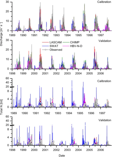
Fig. 2. Observed and predicted daily discharge and daily total N
ex-port during calibration and validation periods for the model cohort.
REA average change is not known beforehand and it is ob-tained iteratively following Giorgi and Mearns (2002). One of the key points of the REA method is thatRB,i or RD,i
are set to 1 wheneverBi or Di are smaller thanε,
respec-tively. Assuming that the probability density function of the change is somewhere between uniform and Gaussian, a 60– 70 % confidence interval is represented by the REA average change plus and minus the weighted root mean square differ-ence (RMSD) such as
RMSD=
PN
i=1Ri· 1TNi−1TN
2
PN
i=1Ri
!1/2
. (3)
3 Results
Time series of simulated and observed discharge as well as TN loads are illustrated in Fig. 2 for both the calibration (1989–1997) and the validation period (1998–2006). Sea-sonal dynamics of observed discharge are well covered by all models, with usually no or only erratic flows from December to April. However, intra-annual discrepancies with observed discharges can be depicted for some models. For example,
Table 2. Model calibration (1989–1997) and validation (1998–
2006) results for runoff.
RMSE (m3s−1) Calibration Validation
LASCAM 1.01 1.11 CHIMP 1.48 1.13
SWAT 1.69 1.24
HBV-N-D 2.31 1.32
SWAT tends to overestimate discharge at the beginning of the wet season in many years, especially in 1989, 2003 and 2004. HBV-N-D has problems to correctly represent discharge at the beginning of the simulation period, strongly underesti-mating discharge in the first three years, which might be at-tributable to a slightly too short spin-up period (2 yr) for this model that led to inadequate initial conditions of water stor-ages. Overall, LASCAM shows the best agreement between simulated and observed discharge for both, the calibration and validation period, apart from the year 2000 where it over-estimates discharge. Calibration and validation metrics are presented in Table 2, as reflected in the time series, LAS-CAM performs clearly better in predicting discharge dur-ing the calibration while HBV-N-D has the largest RMSE of 2.31 m3s−1, more than twice LASCAM’s, as a result of the mismatch from 1989 to 1991. CHIMP and SWAT present in-termediary values during the calibration. The range of RMSE in the ensemble narrows during the validation period. This is due to both LASCAM’s RMSE increasing to 1.11 m3s−1
and HBV-N-D’s reducing to 1.32 m3s−1, while CHIMP and
SWAT also improve their performance.
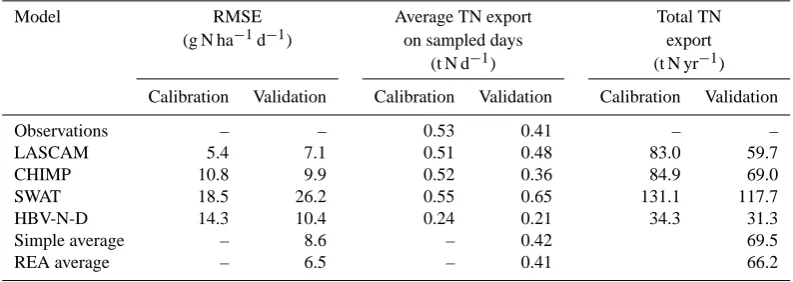
Table 3. Model calibration (1989–1997) and validation (1998–2006) results.
Model RMSE Average TN export Total TN
(g N ha−1d−1) on sampled days export (t N d−1) (t N yr−1) Calibration Validation Calibration Validation Calibration Validation
Observations – – 0.53 0.41 – –
LASCAM 5.4 7.1 0.51 0.48 83.0 59.7
CHIMP 10.8 9.9 0.52 0.36 84.9 69.0
SWAT 18.5 26.2 0.55 0.65 131.1 117.7
HBV-N-D 14.3 10.4 0.24 0.21 34.3 31.3
Simple average – 8.6 – 0.42 69.5
REA average – 6.5 – 0.41 66.2
runoff predictions but has the worst RMSE for TN predic-tions, especially during the validation period. Generally, the models simulated less TN export during validation than dur-ing calibration. The highest TN export is simulated by SWAT with∼131 and∼118 t N yr−1during calibration and valida-tion, respectively. This corresponds to almost 4 times more export than HBV-N-D predictions (∼34 and∼31 t N yr−1). According to Fig. 3 which represents the exceedance proba-bility of daily TN losses simulated by the models, it seems that this difference is due to some rare events of intensive TN export predicted by SWAT. Meanwhile, LASCAM and CHIMP are in a better agreement with each other over the whole period. This is especially true for the simulated export rates of∼83 and∼85 t N yr−1for the calibration period by
LASCAM and CHIMP, respectively. Corresponding values of∼60 and∼69 t N yr−1for the validation period differ a bit
more but are still the most similar amongst all the models. As illustrated in Fig. 3, LASCAM simulated more frequent daily TN exports greater than 1 t N d−1than CHIMP, whereas CHIMP’s higher probability of lower N losses and less fre-quent no flow occurrence explains its higher average yearly TN export.
The validation period also corresponds to the control sce-nario. We therefore present corresponding results for a sim-ple average of the predictions and the REA average in Ta-ble 2. Here, the REA average is only calculated with the reliability criterion as no perturbations have yet been made to our system. The simple average performs with a RMSE equal to 8.6 g N ha−1d−1which is worse than LASCAM but
better than the other three models. However, the correspond-ing average export on sampled days is, at 0.42 t N d−1, closer
to the observed 0.41 t N d−1than any of the single models. Meanwhile, the REA average outperforms all the ensemble members with a value of 6.5 g N ha−1d−1. This represents an improvement of about 10 % compared to LASCAM, the best performing single model. The simulated mean export on sampled days equals the observed mean.
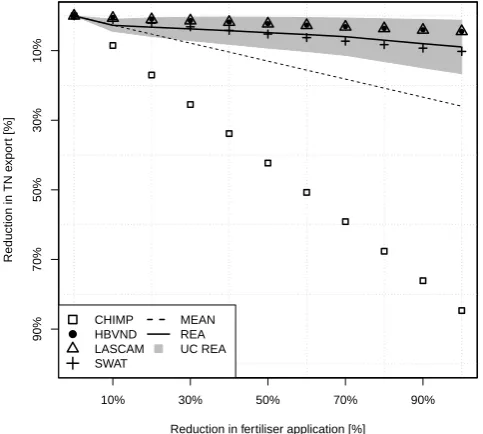
Figure 4 summarises TN export changes for each model. All the members of the ensemble predict the expected
0.0 0.1 0.2 0.3 0.4 0.5 Exceedance probability
0 1 2 3 4 5
Daily TN export [t/d]
LASCAM
CHIMP
SWAT
HBV-N-D
Fig. 3. Exceedance probability of daily TN exports as predicted by
the models during the validation period (1998–2006).
Reduction in fertiliser application [%]
Reduction in TN e
xpor
t [%]
● ● ● ● ● ● ● ● ● ● ●
10% 30% 50% 70% 90%
90%
70%
50%
30%
10%
●
CHIMP HBVND LASCAM SWAT
MEAN REA UC REA
Fig. 4. Evolution of fractional TN export (a proportion of the initial
TN export) with different scenarios of fertilisation reduction.
4 Discussion
Consistently with previous work in hydro-biogeochemical modelling by Breuer et al. (2008), Exbrayat et al. (2010) or Kronvang et al. (2009), discrepancies between model struc-tures (Table 1) driven by a homogeneous dataset of boundary conditions are a source of large predictive uncertainty. In-terestingly, the more lumped models LASCAM and CHIMP seem to perform better in estimating the nutrient losses than the more distributed ones. This may be due to conceptuali-sations of both hydrological and N cycles more adapted to the Ellen Brook conditions. In addition, LASCAM has orig-inally been developed to predict the water, salt and nutrient balances in SW Western Australian catchments including the Ellen Brook (Viney et al., 2000; Zammit et al., 2005). Simu-lation of the water balance greatly impacts nutrient losses and RMSE is more sensitive to the correct timing of peak events. As shown in Table 2, SWAT and HBV-N-D runoff predic-tions are of quality comparable to CHIMP during validation. However, Figs. 2 and 3 as well as Table 3 clearly suggest that SWAT globally overestimates and HBV-N-D underestimates the TN losses, i.e. SWAT good matching of peak events is accompanied by a constant high discharge while HBV-N-D simulates lower flows.
Nonetheless, since our aim is to quantify a relative change in total TN export in response to reductions in fertilisation rates, we do not reject any of the models for our application. Interestingly, the REA average outperforms any of the other simulations in the control case for which we have data to compare with, therefore giving more credit to the approach. The most striking feature in Fig. 4 is the behaviour of the CHIMP model during the scenario analysis. In spite of its
good calibration and validation results, CHIMP simulates a reduction of up to 80 % in TN export while all the other models seem to be more in agreement with a total reduc-tion not higher than 10 % of the current TN export. There-fore, we could attribute the acceptable calibration results of CHIMP as the outcome of a successful curve-fitting exer-cise in which the apparently plausible parameter values are, in fact, incorrect (Wade et al., 2008). Further, because of the outlying position of CHIMP, the simple mean provides a final prediction equivalent to an almost 25 % reduction in nitrogen losses when no fertilisation occurs. However, the trust we can put in this projection is questionable since it is not really in agreement with any of the single projections and its interme-diary position is merely a result of very different but equally weighted projections.
When the agreement between models is introduced into the REA weighting scheme, the converging responses of the LASCAM, SWAT and HBV-N-D models to changed condi-tions provide a significantly different final prediction than the former simple averaging scheme. Similarly to some of the well-calibrated models in Huisman et al. (2009), the outly-ing position of CHIMP decreases its reliability in the final weighing scheme. Conversely, and in spite of their relatively poor ability to match current conditions, SWAT and HBV-N-D “attract” the final averaged prediction by being consistent with each other, and LASCAM, in their relative response to the management scenarios. This results in a final REA av-erage prediction that looks more consistent with most of the single models.
Of course, one could argue that the ensemble approach is not entirely justified in our case because LASCAM is a well-calibrated model that also presents the expected be-haviour during scenario analyses. However, contrary to the other models, LASCAM was primarily developed and tested to simulate water and nutrient fluxes in this particular catch-ment (Viney et al., 2000). In another application case, it is not sure that the chosen model structure would have been devel-oped over several years to predict the hydro-biogeochemical fluxes of the catchment of interest, nor that there would be enough monitoring data to support model quality assess-ment. Similarly, although we agree that CHIMP’s source code needs a thorough inspection in the near future, detec-tion of probable quirks in its structure would not have been possible without comparing its predictions with other models in these scenario analyses.
further step in the innovative direction adopted by our work-ing group as documented in previous contributions (Exbrayat et al., 2010, 2011). Therefore, we consider our results to be very valuable in the frame of hydro-biogeochemical predic-tions (Breuer et al., 2008) and this method could surely be helpful for application cases in which the absence of mon-itoring would make it hard to identify the most appropriate structure (Huisman et al., 2009), such as land management scenarios or prediction in ungauged basins (Sivapalan, 2003). This is especially true since we usually rely on models de-veloped and calibrated for stationary and not changing con-ditions (Milly et al., 2008; Sivapalan et al., 2011).
5 Conclusions
Through our straightforward example of fertilisation rate re-duction we demonstrated the potential advantage of using a multi-model ensemble to lower the risk of relying on a single, maybe subjectively chosen, model structure. This is a real advantage in our application case since the actual effects of different changes are not yet known, making the evaluation of model quality impossible. So far, REA and similar aver-aging schemes have been primarily applied in climate and hydrological sciences and more work is still required in this direction to address their effect on predictions. We therefore see some potential in the ensemble approach in other fields of environmental modelling where the structural uncertainty of models used for predictions is large and rarely addressed.
Acknowledgements. The authors would like to thank the Australian
Bureau of Meteorology for the availability of the climatic data used for model application, as well as the Western Australian Department of Water for providing the runoff and chemical data used for model quality assessment. We further would like to acknowledge the generous funding of this project by the Deutsche Forschungsgemeinschaft DFG, BR2238/5-1. The first author is also funded by the Australian Research Council ARC grant DP110102618.
Edited by: S. Arndt
References
Abramowitz, G. and Gupta, H.: Toward a model space and model independence metric, Geophys. Res. Lett., 35, L05705, doi:10.1029/2007GL032834, 2008.
Arheimer, B. and Brandt, M.: Modelling nitrogen transport and re-tention in the catchments of southern Sweden, Ambio, 27, 471– 480, 1998.
Arheimer, B., Andr´easson, J., Fogelberg, S., Johnsson, H., Pers, C. B. and Persson, K.: Climate change impact on water qual-ity: model results from southern Sweden, Ambio, 34, 559–566, doi:10.1579/0044-7447-34.7.559, 2005.
Arnold, J. G., Srinivasan, R., Muttiah, R. S., and Williams, J. R.: Large area hydrologic modeling and assessment part I:
Model development, J. Am. Water Resour. As., 34, 73–89, doi:10.1111/j.1752-1688.1998.tb05961.x, 1998.
Beven, K.: A manifesto for the equifinality thesis, J. Hydrol., 320, 18–36, doi:10.1016/j.jhydrol.2005.07.007, 2006.
Beven, K. and Freer, J.: Equifinality, data assimilation, and uncer-tainty estimation in mechanistic modelling of complex environ-mental systems using the GLUE methodology, J. Hydrol., 249, 11–29, doi:10.1016/S0022-1694(01)00421-8, 2001.
Breuer, L. and Huisman, J. A.: Assessing the impact of land use change on hydrology by ensemble mod-eling (LUCHEM), Adv. Water Resour., 32, 127–128, doi:10.1016/j.advwatres.2008.10.010, 2009.
Breuer, L., Vach´e, K. B., Julich, S., and Frede, H.-G.: Current con-cepts in nitrogen dynamics for mesoscale catchments, Hydrol. Sci. J., 53, 1059–1074, doi:10.1623/hysj.53.5.1059, 2008. Diekkr¨uger, B., S¨ondgerath, D., Kersebaum, K. C., and McVoy, C.
W.: Validity of agroecosystem models a comparison of results of different models applied to the same data set, Ecol. Model., 81, 3–29, doi:10.1016/0304-3800(94)00157-D, 1995.
Donohue, R., Davidson, W. A., Peters, N. E., Nelson, S., and Jakowyna, B.: Trends in total phosphorus and total nitrogen con-centrations of tributaries to the Swan–Canning Estuary, 1987 to 1998, Hydrol. Process., 15, 2411–2434, doi:10.1002/hyp.300, 2001.
Duan, Q., Sorooshian, S., and Gupta, V.: Effective and efficient global optimization for conceptual rainfall-runoff models, Water Resour. Res., 28, 1015–1031, doi:10.1029/91WR02985, 1992. Exbrayat, J.-F., Viney, N. R., Seibert, J., Wrede, S., Frede, H.-G.,
and Breuer, L.: Ensemble modelling of nitrogen fluxes: data fu-sion for a Swedish meso-scale catchment, Hydrol. Earth Syst. Sci., 14, 2383–2397, doi:10.5194/hess-14-2383-2010, 2010. Exbrayat, J.-F., Viney, N. R., Frede, H.-G., and Breuer, L.:
Prob-abilistic multi-model ensemble predictions of nitrogen concen-trations in river systems, Geophys. Res. Lett., 38, L12401, doi:10.1029/2011GL047522, 2011.
Georgakakos, K. P., Seo, D.-J., Gupta, H., Schaake, J., and Butts, M. B.: Towards the characterization of streamflow simulation uncer-tainty through multimodel ensembles, J. Hydrol., 298, 222–241, doi:10.1016/j.jhydrol.2004.03.037, 2004.
Giorgi, F. and Mearns, L. O.: Calculation of Average, Uncer-tainty range, and reliability of regional climate changes from AOGCM simulations via the “Reliability Ensemble Averaging” (REA) Method, J. Climate, 15, 1141–1158, doi:10.1175/1520-0442(2002)015¡1141:COAURA¿2.0.CO;2, 2002.
Huisman, J. A., Breuer, L., Bormann, H., Bronstert, A., Croke, B. F. W., Frede, H.-G., Graff, T., Hubrechts, L., Jakeman, A. J., Kite, G., Lanini, J., Leavesley, G., Lettenmaier, D. P., Lindstr¨om, G., Seibert, J., Sivapalan, M., Viney, N. R., and Willems, P.: As-sessing the impact of land use change on hydrology by ensem-ble modeling (LUCHEM) III: Scenario analysis, Adv. Water Re-sour., 32, 159–170, doi:10.1016/j.advwatres.2008.06.009, 2009. Krishnamurti, T. N., Kishtawal, C. M., LaRow, T. E., Bachiochi, D. R., Zhang, Z., Williford, C. E., Gadgil, S., and Suren-dran, S.: Improved weather and seasonal climate forecasts from multimodel superensemble, Science, 285, 1548–1550, doi:10.1126/science.285.5433.1548, 1999.
Johns-son, H., Panagopoulos, Y., Lo Porto, A., Reisser, H., Schoumans, O., Anthony, S., Silgram, M., Venohr, M., and Larsen, S. E.: En-semble modelling of nutrient loads and nutrient load partition-ing in 17 European catchments, J. Environ. Monit., 11, 572–583, doi:10.1039/B900101H, 2009.
Legates, D. R. and McCabe Jr., G. J.: Evaluating the use of “goodness-of-fit” Measures in hydrologic and hydrocli-matic model validation, Water Resour. Res., 35, 233–241, doi:10.1029/1998WR900018, 1999.
Lindgren, G. A., Wrede, S., Seibert, J., and Wallin, M.: Nitro-gen source apportionment modeling and the effect of land-use class related runoff contributions, Nordic Hydrol., 38, 317–331, doi:10.2166/nh.2007.015, 2007.
Milly, P. C. D., Betancourt, J., Falkenmark, M., Hirsch, R. M., Kundzewicz, Z. W., Lettenmaier, D. P., and Stouffer, R. J.: Sta-tionarity is dead: whither water management?, Science, 319, 573–574, doi:10.1126/science.1151915, 2008.
Olivera, F., Valenzuela, M., Srinivasan, R., Choi, J., Cho, H., Koka, S., and Agrawal, A.: ArcGIS-swat: A geodata model and GIS Interface for Swat, J. Am. Water Resour. As., 42, 295–309, doi:10.1111/j.1752-1688.2006.tb03839.x, 2006.
Petrone, K. C., Richards, J. S., and Grierson, P. F.: Bioavailability and composition of dissolved organic carbon and nitrogen in a near coastal catchment of south-western Australia, Biogeochem-istry, 92, 27–40, doi:10.1007/s10533-008-9238-z, 2009. Raftery, A. E., Gneiting, T., Balabdaoui, F., and Polakowski, M.:
Using bayesian model averaging to calibrate forecast ensembles, Mon. Weather Rev., 133, 1155–1174, doi:10.1175/MWR2906.1, 2005.
Shamseldin, A. Y., O’Connor, K. M., and Liang, G. C.: Methods for combining the outputs of different rainfall–runoff models, J. Hydrol., 197, 203–229, doi:10.1016/S0022-1694(96)03259-3, 1997.
Sivapalan, M.: Prediction in ungauged basins: a grand challenge for theoretical hydrology, Hydrol. Process., 17, 3163–3170, doi:10.1002/hyp.5155, 2003.
Sivapalan, M., Ruprecht, J. K. and Viney, N. R.: Water and salt balance modelling to predict the effects of land-use changes in forested catchments. 1. Small catchment water balance model, Hydrol. Process., 10, 393–411, doi:10.1002/(SICI)1099-1085(199603)10:3<393::AID-HYP307>3.0.CO;2-#, 1996a. Sivapalan, M., Viney, N. R., and Jeevaraj, C. G.: Water and
salt balance modelling to predict the effects of land-use changes in forested catchments. 3. The large catchment model, Hydrol. Process., 10, 429–446, doi:10.1002/(SICI)1099-1085(199603)10:3<429::AID-HYP309>3.0.CO;2-G, 1996b.
Sivapalan, M., Thompson, S. E., Harman, C. J., Basu, N. B., and Kumar, P.: Water cycle dynamics in a changing environment: Im-proving predictability through synthesis, Water Resour. Res., 47, W00J01, doi:10.1029/2011WR011377, 2011.
Swan River Trust: Ellen Brook Report Card, Perth, West. Aust., Australia, Government of Western Australia, Department of Wa-ter, 2007.
Swan River Trust: Swan Canning Water Quality Improvement Plan, Perth, West. Aust., Australia, Government of Western Australia, Department of Water, 2009.
Viney, N. R. and Sivapalan, M.: Modelling catchment processes in the Swan–Avon river basin, Hydrol. Process., 15, 2671–2685, doi:10.1002/hyp.301, 2001.
Viney, N. R., Sivapalan, M., and Deeley, D.: A conceptual model of nutrient mobilisation and transport applicable at large catchment scales, J. Hydrol., 240, 23–44, doi:10.1016/S0022-1694(00)00320-6, 2000.
Viney, N. R., Bormann, H., Breuer, L., Bronstert, A., Croke, B. F. W., Frede, H.-G., Graff, T., Hubrechts, L., Huisman, J. A., Jakeman, A. J., Kite, G. W., Lanini, J., Leavesley, G., Let-tenmaier, D. P., Lindstr¨om, G., Seibert, J., Sivapalan, M., and Willems, P.: Assessing the impact of land use change on hy-drology by ensemble modelling (LUCHEM) II: Ensemble com-binations and predictions, Adv. Water Resour., 32, 147–158, doi:10.1016/j.advwatres.2008.05.006, 2009.
Vrugt, J. A., Gupta, H. V., Bouten, W., and Sorooshian, S.: A Shuf-fled Complex Evolution Metropolis algorithm for optimization and uncertainty assessment of hydrologic model parameters, Wa-ter Resour. Res., 39, 1201, doi:10.1029/2002WR001642, 2003. Wade, A. J., Jackson, B. M., and Butterfield, D.:
Over-parameterised, uncertain “mathematical marionettes” – How can we best use catchment water quality models? An example of an 80-year catchment-scale nutrient balance, Sci. Total Environ., 400, 52–74, doi:10.1016/j.scitotenv.2008.04.030, 2008. Whitehead, P. G., Lapworth, D. J., Skeffington, R. A., and Wade, A.:
Excess nitrogen leaching and C/N decline in the Tillingbourne catchment, southern England: INCA process modelling for cur-rent and historic time series, Hydrol. Earth Syst. Sci., 6, 455–466, doi:10.5194/hess-6-455-2002, 2002.