https://doi.org/10.5194/gmd-10-2495-2017 © Author(s) 2017. This work is distributed under the Creative Commons Attribution 3.0 License.
Synthesizing long-term sea level rise projections
– the MAGICC sea level model v2.0
Alexander Nauels1,2, Malte Meinshausen1,2,3, Matthias Mengel3, Katja Lorbacher1, and Tom M. L. Wigley4,5 1Australian-German Climate and Energy College, The University of Melbourne, Parkville 3010, Victoria, Australia 2Department of Earth Sciences, The University of Melbourne, Parkville 3010, Victoria, Australia
3Potsdam Institute for Climate Impact Research (PIK), Telegrafenberg, 14473 Potsdam, Germany
4The Environment Institute and School of Biological Sciences, The University of Adelaide, Adelaide, SA 5005, Australia 5Climate and Global Dynamics Division, National Center for Atmospheric Research, Boulder, CO 80307-3000, USA
Correspondence to:Alexander Nauels ([email protected]) Received: 31 August 2016 – Discussion started: 5 October 2016
Revised: 21 June 2017 – Accepted: 22 June 2017 – Published: 30 June 2017
Abstract.Sea level rise (SLR) is one of the major impacts of global warming; it will threaten coastal populations, infras-tructure, and ecosystems around the globe in coming cen-turies. Well-constrained sea level projections are needed to estimate future losses from SLR and benefits of climate pro-tection and adaptation. Process-based models that are de-signed to resolve the underlying physics of individual sea level drivers form the basis for state-of-the-art sea level pro-jections. However, associated computational costs allow for only a small number of simulations based on selected sce-narios that often vary for different sea level components. This approach does not sufficiently support sea level im-pact science and climate policy analysis, which require a sea level projection methodology that is flexible with re-gard to the climate scenario yet comprehensive and bound by the physical constraints provided by process-based mod-els. To fill this gap, we present a sea level model that em-ulates global-mean long-term process-based model projec-tions for all major sea level components. Thermal expansion estimates are calculated with the hemispheric upwelling-diffusion ocean component of the simple carbon-cycle cli-mate model MAGICC, which has been updated and cali-brated against CMIP5 ocean temperature profiles and ther-mal expansion data. Global glacier contributions are esti-mated based on a parameterization constrained by transient and equilibrium process-based projections. Sea level contri-bution estimates for Greenland and Antarctic ice sheets are derived from surface mass balance and solid ice discharge parameterizations reproducing current output from ice-sheet
models. The land water storage component replicates recent hydrological modeling results. For 2100, we project 0.35 to 0.56 m (66 % range) total SLR based on the RCP2.6 scenario, 0.45 to 0.67 m for RCP4.5, 0.46 to 0.71 m for RCP6.0, and 0.65 to 0.97 m for RCP8.5. These projections lie within the range of the latest IPCC SLR estimates. SLR projections for 2300 yield median responses of 1.02 m for RCP2.6, 1.76 m for RCP4.5, 2.38 m for RCP6.0, and 4.73 m for RCP8.5. The MAGICC sea level model provides a flexible and efficient platform for the analysis of major scenario, model, and cli-mate uncertainties underlying long-term SLR projections. It can be used as a tool to directly investigate the SLR implica-tions of different mitigation pathways and may also serve as input for regional SLR assessments via component-wise sea level pattern scaling.
1 Introduction
mag-nitude of total sea level rise (SLR) will strongly depend on the amount of anthropogenic greenhouse gases (GHGs) emitted to the atmosphere during the 21st century and the corresponding physical responses of the major SLR drivers (Horton et al., 2014). Future GHG emissions are therefore a main uncertainty source when trying to project SLR tra-jectories. SLR uncertainties are further increased by struc-tural differences of the underlying process-based models for the individual SLR contributions and limited process under-standing, like the behavior of polar ice shelves in a warm-ing world (Nicholls and Cazenave, 2010). To assess major parts of these scenario and model uncertainties, we extend the widely used simple carbon-cycle climate model MAG-ICC (Meinshausen et al., 2011a, 2009; Wigley et al., 2009; Wigley and Raper, 2001) to comprehensively model global SLR. This MAGICC sea level model has been designed to emulate the behavior of process-based sea level projections presented in the fifth IPCC Assessment Report (Church et al., 2013a), with thorough calibrations for each major sea level component. It is intended to serve as an efficient and flexible tool for the assessment of multi-centennial global SLR. In the following section, we motivate and explain the key concepts underlying the MAGICC sea level model. Section 2 covers the detailed model description and Sect. 3 provides key re-sults. In Sect. 4, we discuss the capabilities of the presented sea level emulator and shine a first light on potential applica-tions.
Motivation
Future sea level is modeled with varying degrees of com-plexity. Process-based modeling represents the physically most comprehensive but also computationally most expen-sive approach to project SLR. It is based on Atmosphere– Ocean General Circulation Models (AOGCMs) and spe-cialized glacier, ice-sheet and groundwater models that dy-namically simulate sea level changes resulting from natu-ral and anthropogenic forcings. The main sea level output from AOGCMs is the thermosteric ocean response, mostly diagnosed with post-simulation adjustments to compensate Boussinesq approximation effects (Griffies and Greatbatch, 2012). Process-based glacier and ice-sheet models are gener-ally run separately or “offline” and receive important bound-ary conditions either from observational data, AOGCMs, or regional climate model input (Rae et al., 2012; Pattyn et al., 2012). Due to the complexity of the physical processes re-quired to capture the dynamical response of each individ-ual component, this SLR modeling approach is not feasible for efficient multi-centennial and multi-scenario research de-signs. It is mainly used to improve our physical understand-ing of the individual SLR components. The need for more efficient tools to project long-term SLR has led to the devel-opment of alternative approaches.
In the 1980s, first semi-empirical models (SEMs), which estimate global sea level changes based on the evolution
of global-mean temperature, were introduced together with early approaches to model thermal expansion based on simplified ocean processes (Gornitz et al., 1982). Gener-ally, SEMs establish statistical relationships between ob-served/reconstructed global-mean temperature or radiative forcing changes and observed/reconstructed global-mean sea level changes. Assuming that such relationships do not change in the future, they are used to estimate future SLR from projected global temperature/forcing changes (Rahm-storf, 2007; Vermeer and Rahm(Rahm-storf, 2009; Jevrejeva et al., 2010; Kopp et al., 2016). Therefore, these SEMs do not cal-culate sea level by resolving the underlying physical pro-cesses. This approach generated considerable scientific de-bate and was not included in latest IPCC estimates (Or-lic and Pasaric, 2013; Storch et al., 2008; Church et al., 2013a). The computational efficiency of this method, how-ever, made it attractive to applied research questions, like in-vestigating the global-mean SLR response for different cli-mate targets (Schaeffer et al., 2012). Recently, this method has been developed further and was applied to individual sea level components (Mengel et al., 2016). SLR projections are also provided based on expert elicitations (Horton et al., 2014). Furthermore, sea level expert judgments have been combined with statistical models synthesizing sea level pro-jections for individual components (Kopp et al., 2014). Other studies have used an extended suite of methods, analyzing paleoclimatic archives, modeling parts of the SLR response with a reduced complexity model, and deriving future projec-tions for land-ice contribution-based semi-empirical consid-erations (Clark et al., 2016). The growing efforts in the sea level modeling community to provide fully transparent and freely available model code are reflected by the recent intro-duction of a transparent, simple model framework to estimate regional sea levels (Wong et al., 2017). Previous MAGICC versions also provided SLR estimates based on simplified pa-rameterizations for selected components (Wigley and Raper, 1987, 1992, 2005; Wigley, 1995).
Intercompari-son Project (CMIP5) (Taylor et al., 2012). It mimics process-based sea level responses for the seven main sea level compo-nents with thoroughly calibrated parameterizations that ex-tend global sea level projections to 2300. Integration of the sea level model into MAGICC ensures a consistent treatment of future SLR and its uncertainties along the full chain from emissions to atmospheric composition, to temperature to sea level. With the option to run large ensembles in a probabilis-tic setup, the MAGICC sea level model allows one to explore the scenario and model uncertainty space and directly inves-tigate SLR responses associated with mitigation pathways that are not covered by the standard RCP scenarios (Moss et al., 2010). In addition, the MAGICC global SLR projec-tions could be used for calculating regional SLR information by using them as input for pattern scaling approaches (Per-rette et al., 2013).
2 Model description
The MAGICC sea level emulator (Fig. 1) has been developed as an extension to the widely used MAGICC model version 6 (Meinshausen et al., 2011a, b). The MAGICC ocean model has been revised and calibrated with available CMIP5 ocean temperature and thermal expansion data. The updated MAG-ICC ocean provides the basis for our thermal expansion pa-rameterization based on Lorbacher et al. (2015). Parameter-izations for global glacier, Greenland surface mass balance (SMB), Antarctic SMB, and Greenland solid ice discharge (SID) have been calibrated against selected process-based projections for the corresponding SLR components. The lin-ear response function approach for the Antarctic SID com-ponent presented in Levermann et al. (2014) was adapted to satisfy MAGICC model specifications. In addition, we have implemented the option to include land water SLR contri-bution estimates based on Wada et al. (2012, 2016), with an extension until 2300.
2.1 MAGICC ocean model update and thermal expansion
MAGICC is based on a hemispheric upwelling-diffusion en-trainment ocean model with depth-dependent areas for each of its 50 ocean layers (Meinshausen et al., 2011a). In this study, we provide a first series of updates for MAGICC ver-sion 7, which will be consistent with the ensemble output of CMIP5 (Taylor et al., 2012). The upwelling velocity is variable in MAGICC and the model conserves the upwelling mass flux through layer-specific entrainment which is pro-portional to the area decrease from the top to the bottom of each layer. To avoid overestimation of ocean heat uptake for higher warming scenarios, the ocean routine includes a warming-dependent vertical diffusivity term which leads to reduced heat uptake efficiency for higher warming (Meshausen et al., 2011a). In MAGICC6, the air temperature
in-creases were assumed proportional to the mixed-layer ocean temperatures. A proportionality constant α (default value: 1.25) is used in earlier versions of MAGICC to account for diminishing sea-ice extent in the Arctic, exposing a larger area of the (relatively warm) surface ocean waters as warm-ing progresses with time. Here, we replace this constant fac-tor by a term that takes into account the fact that this ampli-fying effect will itself diminish as the Arctic sea-ice retreat is bound by the limit of a sea-ice-free ocean in summer. The chosen functional form initially assumes a simple linear am-plification (as in MAGICC6), and then progresses asymptot-ically towards a constant offset between the surface air tem-perature and top ocean-layer warming. This new exponential adjustment term relates hemispheric air temperature change
1TxAto hemispheric mixed-layer ocean temperature change 1TxO,1as follows:
1TxA=1TxO,1+η
1−e−γ 1TxO,1. (1) For largeγ 1TxO,1, the new sea-ice adjustment term moves towards a constant offsetηbetween surface air temperature warming 1TxA and mixed-layer ocean warming 1TxO,1. However, the surface air temperature warming initially ap-proximates 1TxA=1TxO,1(1+ηγ ) for small γ 1TxO,1, with(1+ηγ )representing the old MAGICC6 proportion-ality coefficientα. The sea-ice adjustment parametersηand
γ are optimized together with other selected parameters for every CMIP5 model included in the MAGICC ocean model calibration (see Sect. 2.6). The parameter sets are optimized to represent the depth-dependent potential ocean tempera-ture (thetao) responses from 36 CMIP5 models (see Ta-ble 1). The tuned model captures ocean-layer-specificthetao
change and related vertical redistribution characteristics of individual CMIP5 models, both indicators for overall ocean heat uptake behavior. Net ocean heat uptake can be robustly translated into thermal expansion (Kuhlbrodt and Gregory, 2012). Therefore, we can define the thermosteric response as the vertical sum of the layer-specific thetao anomalies multiplied by a corresponding thermal expansion coefficient
αwhich is weighted by the specific ocean-layer area. The thermal expansion coefficientα captures all relevant prop-erties of seawater (potential seawater temperature, salinity, and pressure) that determine the corresponding sea level re-sponse (Griffies et al., 2014). For MAGICC, a simplified thermal expansion coefficient representation was developed, which is solely based onthetaoand pressure (Raper et al., 2001; Wigley et al., 2009). Recently, Lorbacher et al. (2015) have updated this parameterization to match CMIP5 thermal expansion behavior. We build our parameterization on Lor-bacher et al. (2015) and calculate the thermal expansion co-efficients for every MAGICC depth with the following poly-nomial ofθandp:
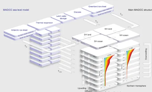
Figure 1.Schematic of the MAGICC sea level model structure and the driving MAGICC hemispheric upwelling-diffusion energy balance core. Heat is transported through the oceans by downwelling and corresponding layer entrainment, upwelling, diffusion, and the exchange between the hemispheres. Ocean mixed layer is denoted MXL, depth-dependent ocean areas are shown by smaller ocean layers towards the ocean bottom. Illustrative potential ocean temperature warming profiles that feed into the layer-dependent thermal expansion module are sketched for both hemispheres. Ocean and air temperature fluxes (TOCN,TGL) relevant for the sea level model as well as other major energy
fluxes are shown as arrows. Figure adapted from Meinshausen et al. (2011a).
−0.019263p)+c3θ2(10.41−1.338p) +c4p−c5p2
10−6. (2)
The hemispheric layer-specificthetaovaluesθzare processed
for every time step withθ0=θz,θ1=θ02, andθ2=
θ03
6000, as-suming a mean maximum ocean depth of 6000 m. The ocean depth profile, z, is translated into the pressure profile p= 0.0098(0.1005z+10.5 exp−35001.0z−1.0, with 3500 m as the mean ocean depth. For each of the 36 MAGICC CMIP5 ocean parameter sets, the corresponding calibration parame-tersc0−5are taken from Table S2 in Lorbacher et al. (2015). It is the combination of the CMIP5 MAGICC ocean update with the matching thermal expansion parameters that allows us to estimate 36 unique thermal expansion responses based on the selected ensemble of CMIP5 models. Our method does not cover all the spatial heterogeneity effects of ther-mal expansion that are seen in the three-dimensional CMIP5 fields. Therefore, we apply a model-specific scaling coeffi-cientφto the thermosteric estimates for each ocean layer to further improve the fit between the aggregated thermal
ex-pansion from the calibrated MAGICC ocean model and the CMIP5 thermosteric SLR (zostoga) estimates (see Sect. 2.6 for more details).
2.2 Global glaciers
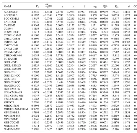
Table 1.MAGICC ocean model calibration results with optimal sets of ocean and thermal expansion calibration parameters for the available CMIP5 models. Calibration parameters are introduced in Sect. 2.6. Goodness-of-fit (GOF) results are given as weighted residual sum of squares (RSS) divided by the number of calibrated model years (weight potential ocean temperature [K]: 10; weight thermal expansion [mm]: 0.001). The optimal set for the mean response of the calibration data is given at the bottom of the table.
Model Kz
dKztop
dT η γ β w0
1wt
wt Twt φ GOF
ACCESS1.0 4.3846 −1.3441 2.4191 0.2954 0.1997 0.0678 0.9999 1.9021 1.1141 0.11
ACCESS1.3 0.1792 −0.0249 4.5743 0.0806 0.0598 9.959 0.2044 3.0533 1.1277 0.08
BCC-CSM1.1 1.3457 0.0701 2.223 0.2245 0.2348 0.0100 0.9506 16.417 1.0303 0.11
BNU-ESM 1.9336 −0.4034 3.5734 0.2422 0.6824 2.9546 0.0010 4.5004 1.2220 0.13
CanESM2 0.9065 0.2868 5.0000 0.1132 0.1259 1.171 0.7481 8.1589 1.0857 0.16
CCSM4 1.1155 0.2327 1.6218 0.3368 0.0132 1.2702 0.3359 1.5202 1.0321 0.15
CESM1-BGC 1.1713 −0.0654 3.2018 0.1302 0.1024 9.986 0.223 3.8928 1.0533 0.03
CESM1-CAM5 0.1000 0.8004 2.5411 0.2834 0.0767 1.9277 0.7618 16.873 1.0993 0.13
CMCC-CESM 0.4599 −0.0209 1.8620 0.2551 0.0100 10.000 0.4610 9.4486 1.1590 0.13
CMCC-CM 1.4137 −0.4317 1.0552 0.9129 0.2519 1.9925 0.9999 19.599 0.9382 0.10
CMCC-CMS 0.1000 −0.7989 4.9992 0.0807 0.1531 9.9999 0.2939 4.7474 0.9858 0.05
CNRM-CM5 0.1377 0.1547 3.2070 0.1776 0.4134 0.5078 0.8680 1.3343 1.0254 0.20
CNRM-CM5-2 1.3200 −0.2081 5.0000 0.1146 0.1037 0.6386 0.8098 1.7782 1.4547 0.05
CSIRO-Mk3.6.0 2.0085 −0.0361 3.7756 0.1510 0.0137 0.0117 0.1865 17.812 1.0633 0.49
EC-EARTH 2.5850 −0.6157 4.9892 0.1077 0.2489 2.4364 0.0720 19.999 1.0624 0.05
GFDL-CM3 0.1000 0.3796 5.0000 0.1638 0.0599 2.9073 0.3461 2.3735 1.1692 0.18
GFDL-ESM2G 2.6329 −1.4040 2.1535 0.2304 1.0000 2.2037 0.8837 20.000 1.3555 0.15
GFDL-ESM2M 2.9547 1.0000 4.9372 0.1387 0.1479 0.0101 0.5316 7.4830 1.1790 0.11
GISS-E2-H 1.2987 0.3002 1.5682 0.4334 0.0334 0.5996 0.9527 2.4943 1.1256 0.07
GISS-E2-HCC 0.1000 1.0000 1.4129 0.6907 0.3571 3.7715 0.9091 17.974 1.0928 0.11
GISS-E2-R 0.9151 0.9383 1.6601 0.4458 0.1069 1.0556 1.0000 1.5897 1.0861 0.17
GISS-E2-RCC 4.9680 −1.0529 1.484 0.5898 0.1609 1.3509 0.2843 1.3137 1.1696 0.12
HadGEM2-CC 0.4727 −0.0493 2.8069 0.1638 0.5988 4.6183 0.0246 1.2449 1.3297 0.07
HadGEM2-ES 0.6165 0.0620 3.4649 0.2123 0.3212 2.9456 0.2779 2.3299 1.1488 0.39
IPSL-CM5A-LR 1.0928 −0.0191 3.1337 0.1181 0.2414 1.8789 0.3740 11.705 1.0677 0.10
IPSL-CM5A-MR 1.0047 −0.0643 1.5549 0.3573 0.9473 0.7214 1.0000 15.414 1.0472 0.09
IPSL-CM5B-LR 1.6262 0.0318 5.0000 0.1234 0.0262 6.5424 0.1259 12.950 1.2550 0.05
MIROC5 2.2396 0.5792 4.9999 0.0961 0.4486 0.0100 0.1234 2.8327 1.1048 0.15
MIROC-ESM 0.6896 0.1877 2.0219 0.4933 0.2884 1.4103 0.9501 3.6729 1.1383 0.12
MIROC-ESM-CHEM 0.9997 −0.5891 1.1388 1.1193 0.0254 9.6999 0.3022 4.4868 1.1277 0.05
MPI-ESM-LR 1.7898 −0.0385 3.2976 0.2319 0.8504 1.1209 0.2792 2.1975 1.2154 0.33
MPI-ESM-MR 2.0752 −1.2640 1.4401 0.5752 0.0510 10.000 0.5349 8.2459 1.1122 0.06
MPI-ESM-P 1.3946 −0.4808 4.4931 0.0898 0.0389 10.000 0.2498 3.9468 1.2927 0.07
MRI-CGCM3 1.4610 0.2543 4.2439 0.1300 0.1760 5.9552 0.0071 2.4876 1.1478 0.05
NorESM1-M 1.3714 0.4972 1.404 0.4805 1.0000 3.0676 0.2752 2.5603 1.1744 0.11
NorESM1-ME 2.8281 0.6425 2.8026 0.1382 0.2966 10.000 0.0266 15.706 1.1203 0.08
Mean 1.3547 −0.7115 1.7022 0.3602 0.5515 9.9876 0.2469 4.2944 0.8823 0.05
data. Changes in glacier volume are derived with the help of volume–area scaling methods. In the follow-up study (Marzeion et al., 2014), 2300 estimates of transient glacier mass dynamics forced by 15 CMIP5 temperature and pre-cipitation fields were complemented by equilibrium global glacier projections in response to long-term warming levels from 1 to 10◦C. These two experimental setups projecting transient and equilibrium glacier SLR contributions form the basis of the glacier component that has been implemented in the MAGICC sea level model. We include Randolph Glacier Inventory 4.0 (RGI 4.0) updates on regional glacier mass loss
(Pfeffer et al., 2014). The selected parameterization is based on the assumption that global glacier melt is proportional to the remaining volume susceptible to melt (at the current global temperature) times the melt forcing. This melt forcing is expressed by the temperature difference between current temperature and the temperature that would be expected if the currently remaining glacier volume was in equilibrium. Thus, we apply the following functional form to relate the global glacier SLR response GLt to the remaining global
glacier volume as well as the temperature forcing: GLt=GLt−1+κ Veq−Vcum
Tt−Teq
ν
with calibration parametersκ andνandVeqbeing the equi-librium glacier volume change that would result from warm-ing level Tt. This value is interpolated from the Marzeion
et al. (2014) glacier equilibrium response data. Vcumis the cumulative glacier volume change since the year 1850.Teqis the inverse function of the equilibrium glacier responseVeq toTtand gives the temperature that would lead to the glacier
volume changeVcumin terms of a theoretical equilibrium re-sponse.
2.3 Greenland ice sheet
The Greenland contribution to SLR increased rapidly dur-ing the last decades of the 20th century (Vaughan et al., 2013). Regional atmospheric and ocean warming has trig-gered widespread surface melt (Fettweis et al., 2011) and solid ice discharge (Joughin et al., 2012). An increasingly negative SMB and a growing SLR contribution from SID, which captures accelerating ice stream flow and more fre-quent calving events due to warmer ocean temperatures, have been identified to be responsible for about half of the ob-served mass loss each (van den Broeke et al., 2009; Khan et al., 2015). The Greenland ice sheet is expected to be-come one of the largest SLR contributions in the future (Huy-brechts et al., 2011), with potentially irreversible ice-sheet loss for scenarios of persistent and strong warming (Robin-son et al., 2012; Levermann et al., 2013). In the following, we present SMB and SID parameterizations that have been im-plemented and calibrated in the MAGICC sea level model. 2.3.1 Surface mass balance
The mass balance at the surface of the Greenland ice sheet is predominantly determined by the accumulation of snow-fall in winter and runoff through melting in summer. Con-tinuing global warming will influence the SMB through both increased snowfall and increased melting (Gregory and Huy-brechts, 2006). As melting is expected to increase more strongly than snowfall, SMB losses will likely dominate fu-ture Greenland contributions to SLR (Church et al., 2013a; Goelzer et al., 2013). Regional surface air temperatures are the primary driver of these projected SMB changes if we as-sume future precipitation changes over Greenland to be scal-able with rising temperatures (Fettweis et al., 2013; Frieler et al., 2012). Regional atmospheric temperatures are closely linked to the global-mean surface air temperaturetas. We uti-lize this link for our sea level component by relating twotas -dependent terms to capture the long-term SMB sea level re-sponse. In the parameterization, the SMB response totascan vary from either being approximated as scaling linearly, or nonlinearly with exponent ϕ, or as a combination of both. The calibration procedure chooses the optimal balance of the linear and nonlinear terms. Furthermore, the surface melt contribution is damped by diminishing ice availability for high warming scenarios and eventually becomes zero when
all available ice is melted. Hence, the cumulative Greenland SMB SLR contribution GISSMBt at time stept can be written as
GISSMBt =GISSMBt−1 +υ χ Tt+(1−χ )Ttϕ
1−GIS SMB
t−1
GISSMBmax
!0.5
. (4)
The maximum Greenland ice volume available for surface melt GISSMBmax is about 7.36 m (Bamber et al., 2013). The over-all temperature sensitivity is denoted byυand the choice of
ϕsets the degree of nonlinearity, whileχdetermines the rel-ative magnitude of the linear and nonlinear terms. We cali-brate the three parametersυ,χ, andϕ with reference data from Fettweis et al. (2013). Their process-based Greenland SMB projections until 2100 are based on the regional climate model Modele Atmospherique Regional (MAR), which is coupled to the soil-ice-snow-vegetation-atmosphere transfer scheme. The MAR model is forced by CMIP5 data for tem-perature, wind, humidity, and surface pressure. Comparing the MAGICC Greenland SMB response to millennial pro-jections of Greenland ice-sheet sea level contributions (Huy-brechts et al., 2011; Goelzer et al., 2012) indicates that the functional form of our SMB parameterization will hold for multi-centennial projections at least until 2300.
2.3.2 Solid ice discharge
GISSIDt at time steptbeing: GISSIDt =s
GISoutletmax −GISoutletVdis(t ) (5) with GISSIDt defined as the difference of the initial maximum ice volume susceptible to discharge and the remaining ice volume available for discharge at time stept. Maximum ice volume, GISoutletmax , and remaining ice volume at time step t, GISoutletVdis(t ), are determined for the four main Greenland outlet glaciers. By applying the scaling factors=5, the sea level contribution is then scaled up to the entire Greenland ice sheet. Fort=0, GISoutletVdis(t=0)=GISoutletmax . The remaining ice volume susceptible to discharge at time stept, GISoutletVdis(t ), has the following function form:
GISoutletVdis(t )=GISoutletVdis(t−1)
−max0, %GISoutletVdis(t−1)eT(t−1) (6)
with the annual discharge being the product of the discharge sensitivity%, the SID volume GISoutletVdis(t−1) available at time stept−1, and an exponentialtasterm, which is dependent on a temperature sensitivity. We have calibrated%,, and the maximum SID outlet glacier volume GISoutletmax based on the projected minimum and maximum contributions for dynamic retreat and thinning for scenarios SRES A1B and RCP8.5, shown in Fig. 3e of Nick et al. (2013). An upper limit of the potential Greenland SID discharge contribution has not been clearly defined yet (Goelzer et al., 2013; Price et al., 2011). We include the maximum SID outlet glacier volume suscep-tible to discharge GISoutletmax in our calibration. Applying the scaling suggested by Church et al. (2013a), our total Green-land SID maximum ice discharge volumes amount to around 180 and 268 mm SLE for the minimum and maximum cases presented in Nick et al. (2013). For comparison, Winkelmann and Levermann (2012) obtained 420 mm for the ice-dynamic Greenland sea level contribution, indicating, however, that the actual amount might be significantly smaller. For high warming scenarios, our SID projections deplete GISoutletmax be-fore the year 2300, which causes the annual Greenland SID sea level contribution to drop to zero.
2.4 Antarctic ice sheet
Air temperatures over the Antarctic ice sheet are generally much colder than over the Greenland ice sheet. They will be too low to cause wide-spread surface melting, even un-der strong global warming (Church et al., 2013a). Only pe-ripheral, low-lying glaciers, especially around the Antarctic Peninsula are susceptible to retreat through increased ab-lation (Krinner et al., 2006). A warmer atmosphere over Antarctica will however hold more moisture, leading to higher snowfall. This effect is expected to lead to a posi-tive SMB through snow accumulation and, thus, a slightly negative SLR contribution (Bengtsson et al., 2011; Gregory
and Huybrechts, 2006). The main driver of Antarctic ice loss and a resulting positive sea level contribution is the increased melting of ice shelves through warmer ocean waters (Joughin et al., 2012; Bindschadler et al., 2013). SID will be the domi-nant SLR contribution of Antarctica, with increasing ocean temperatures causing basal melt in marine-based ice-sheet sectors, potentially even triggering marine ice-sheet instabili-ties and irreversible ice loss (Huybrechts et al., 2011; Joughin et al., 2014). We implemented parameterizations capturing both the Antarctic SMB and the SID contributions to SLR in the MAGICC SLR mode. They are presented below. 2.4.1 Surface mass balance
Positive Antarctic SMB anomalies under all warming sce-narios lead to consistently negative contributions to global sea level for the 21st century. Similar to Greenland, a strong (but different) link exists between future Antarctic SMB and global-mean surface air temperaturetas. Several stud-ies confirmed the Clausius–Clapeyron equation-based expo-nential relationship between atmospheric warming and SMB accumulation. The values range from 3.7 %◦C−1 (Krinner et al., 2006) up to around 7 %◦C−1(Bengtsson et al., 2011), with most recent estimates based on a large ensemble of climate models pointing to about 5 %◦C−1 (Frieler et al., 2016). Ligtenberg et al. (2013) has been one of the few stud-ies using regional climate simulations to assess Antarctic SMB changes beyond 2100, without accounting for climate– ice-sheet feedbacks however. Their assessment is based on the regional atmospheric climate model RACMO2 (Lenaerts et al., 2012) and the two global climate models ECHAM5 (Roeckner et al., 2003) and HadCM3 (Johns et al., 2003) that have been forced by two comparably moderate emission scenarios (SRES A1B and ENSEMBLES E1), leading to a 2200 Antarctic warming of 2.4–5.3◦C. Results show SMB increases of 8–25 %, which translate into a global sea level drop of 73–163 mm. We select these projections as reference for our SMB parameterization. Due to the expected strong SMB link totas, we have chosen a simple functional form that relates the annual Antarctic SMB sea level contribution to this primary driver:
AISSMBt =AISSMBt−1 +ξ ρTt+(1−ρ)Ttσ
. (7)
by idealized scenarios doubling or quadrupling atmospheric CO2concentration levels (Vizcaíno et al., 2010; Huybrechts et al., 2011). Results from these studies show ice mass gains due to additional snowfall for more than 500 years after the start of the experiments, e.g., see Fig. 7 in Huybrechts et al. (2011).
2.4.2 Solid ice discharge
Improved process understanding has allowed for a first as-sessment of the Antarctic dynamic ice-discharge contribution to SLR in the fifth IPCC Assessment Report (Church et al., 2013a). Antarctic SID has the potential to supersede all other sea level contributions because of the vast ice masses acces-sible for warm ocean waters and susceptible to self-amplified retreat (DeConto and Pollard, 2016). Loss of these ice masses alone would eventually lead to several meters of global SLR (Bamber et al., 2009). Recent observations and modeling suggests that the process of self-sustained retreat has already begun and will dominate over the slower adjustments totas
and precipitation changes across the Antarctic continent on decadal to centennial timescales (Joughin et al., 2014; Rignot et al., 2014; Favier et al., 2014). Levermann et al. (2014) con-volved the responses from five different Antarctic ice-sheet models to basal melt forcing as used in the SeaRISE project (Bindschadler et al., 2013) with a large set of MAGICC tem-perature projections for the full suite of RCP scenarios. In their study, the projected global-meantassignal is converted into subsurface ocean temperatures that are translated into basal melt forcing. The melt forcing is then convolved with individual response functions for the Amundsen Sea, Ross Sea, Weddell Sea, and East Antarctic sectors. This approach is well-suited for the MAGICC sea level model implementa-tion because it relates the ice-sheet response directly totas. We implement a step-wise convolution routine in the MAG-ICC SLR model, which allows us to process the response functions for the different sectors. The total SLR contribu-tion from Antarctic SID, AISSID, can be written as the sum of the contributions from the individual sectors:
AISSID= 4
X
n=1
t Z
0
Fn(τ )Rn(t−τ )dτ. (8)
The sector-specific basal melt forcing Fn is the product of
the basal melt sensitivityψand the sector-specific subsurface ocean temperature anomaly dTOCN. The region-specific ice-sheet response functionRn(t−τ )is based on linear response
theory (Winkelmann and Levermann, 2012). The basal melt forcingF is the product of the basal melt sensitivityψand the sector-specific subsurface ocean temperature anomaly dTOCN. Starting in 1850, Levermann et al. (2014) derived the latter from the projected annual MAGICC global-meantas
anomalies via ocean temperature scaling and a time delay between surface and ocean subsurface warming. We adopt all relevant melt forcing parameters from Levermann et al.
(2014). They determined these parameters either through cal-ibrations against 19 CMIP5 models or adopted them from the existing literature, such as the basal melt sensitivities ranging from 7 to 16 m a−1K−1(Holland et al., 2008; Payne et al., 2007; Jenkins, 1991). The response functions are de-rived for 500 years and cover the time frame of their source experiments described in Bindschadler et al. (2013). We pro-vide Antarctic SID projections up to the year 2300. For the MAGICC component, it is only response functions from the three ice-sheet models that have an explicit representation of ice-shelf dynamics that is included, namely PennState-3D (Pollard and DeConto, 2012), PISM (Winkelmann et al., 2011; Martin et al., 2011), and SICOPOLIS (Sato and Greve, 2012). The response functions presented by Levermann et al. (2014) and implemented here do not account for all ice-sheet processes and feedbacks. Thus, the Antarctic SID estimates provided by the MAGICC sea level model may underesti-mate the actual Antarctic SID sea level response.
2.5 Land water storage
LWS contribution to a theoretical maximum LWS volume that can be depleted. No distinction is made between differ-ent climate scenarios for the post-2100 LWS extension due to the limited process understanding and the associated large uncertainties (Church et al., 2013a). Hence, we implement the revised Wada et al. (2012) estimates until 2100 and apply the following post-2100 LWS parameterization:
LWSt=LWSt−1+LWSconst
1−LWSt−1−LWS2100 LWSmax−LWS2100
0.5
. (9)
The maximum LWS volume LWSmaxhas not been quantified yet de Graaf et al. (2014). However, Gleeson et al. (2015) quantified the amount of modern groundwater, which is de-fined as less than 50-year-old groundwater located in the top 2 km of the continental crust. This type of groundwater dom-inates the interaction with general hydrological cycle and the climate system. It is also the most accessible for land use (Gleeson et al., 2015). We here define LWSmax as the total amount of available modern groundwater, which has been estimated to be around 350 000 km3, roughly translating to 1000 mm SLE.
2.6 Model calibration
For the MAGICC ocean model calibration, we use two CMIP5 variables for our reference dataset: ocean poten-tial temperatures (thetao) and thermal expansion (zostoga). Ocean-depth-specific thetao time series are extracted for a total of 36 CMIP5 models, which have been running pre-industrial control (pictrl), historical, some or all of the RCP experiments as well as the idealized 1 % CO2 per year in-crease (1pctCO2) experiments. Each individual model output is converted into hemispheric annual-meanthetaodepth pro-file time series that are then vertically interpolated to match the MAGICC ocean-layer depths. We combine historical and RCP runs to create layer-specific time series from 1850 to 2100 or 2300 depending on the experiment lengths of the in-dividual CMIP5 model runs. Ocean temperature data avail-able from the CMIP archives are subject to drift because the time scales for the ocean to adjust to external forcing are much longer than the length of the control experiments (Taylor et al., 2012; Gupta et al., 2013). Individual model drifts have been identified based on the respectivepictrlruns. The full linear trend from thepictrlexperiments has been re-moved from the historical plus RCP and1pctCO2scenario time series.
The initialthetaoprofiles are prescribed for every CMIP5 model calibration as well as the respective depth-dependent ocean area fractions. We incorporate zostogaestimates for each of the 36 CMIP5 ensemble members by detrending the times series with the full linear trend of thepictrlruns. To en-sure a full CMIP5-consistent calibration setup, we constrain MAGICC for every CMIP5 model optimization by prescrib-ing the correspondprescrib-ing model-specific annual global-mean
surface air temperaturetas. Previous studies have shown that calibration methods for highly parameterized simple models do successfully show global convergence, even with a large number of free parameters (Hargreaves and Annan, 2002; Meinshausen et al., 2011a). Here, we select all MAGICC pa-rameters, which directly determine the ocean-layer-specific potential ocean temperature and corresponding thermal ex-pansion responses. These nine parameters drive the band routine of the hemispheric upwelling-diffusion ocean model. The vertical thermal diffusivity,Kz, its sensitivity to
global-mean surface temperatures at the mixed-layer boundary, dKztop
dT , the sea-ice adjustment parametersηandγ described
above, the initial upwelling ratew0, the ratio of changes in the temperature of the entraining waters to those of the po-lar sinking watersβ, the ratio of variable to fixed upwelling
1wt
wt , and the corresponding threshold temperatures that lead
to constant upwelling rates, namelyTwt, and the global
ther-mal expansion scaling coefficientφ. The minimum vertical diffusivityKz,min is set to 0.1 cm2s−1, as stated in Mein-shausen et al. (2011a). This value represents the lower bound for the calibration ofKz. More details on the individual
pa-rameters can be found in Meinshausen et al. (2011a) except for the sea-ice adjustment variables described in Sect. 2.1. For every CMIP5 model, this suite of calibration parameters is optimized based on the scenario-specific CMIP5 thetao
The calibration procedures for the other SLR components also optimize the specific parameters listed in Tables 2 to 5 based on the Nelder–Mead Simplex method with a termina-tion tolerance of 10−8for a change in RSS during the last iteration. For an overview of all relevant variables and cal-ibration parameters please see Table A1. All the remaining SLR components use reference SLE contributions in mil-limeters for the respective optimizations. For the glacier con-tribution, the MAGICC sea level response is fitted to the tran-sient Marzeion et al. (2014) projections. The free parame-ters κ andν are calibrated for each of the 14 CMIP5 ref-erence models and their respective combined historical and RCP simulations, starting in 1850. Corresponding CMIP5 global-meantasprojections are prescribed in the MAGICC model to ensure consistency with CMIP5. We use a subset of the model-specific 1965–2100 projections made available by Fettweis et al. (2013) to calibrate the parameterization for the Greenland SMB contribution. In total, 24 CMIP5 models are selected based on the availability of CMIP5tas projec-tions for the scenarios RCP4.5 and RCP8.5. We then pre-scribe these global-mean tastime series for the calibration procedure of the three parametersυ,χ, andϕ. Calibration data for the Greenland SID component is only available for one GCM, ECHAM5. For the optimization of the parame-ters%,, and GISoutletmax , global-meantasruns for SRES A1B and RCP8.5 are used with 2200 extensions, repeating the last decade of the 21st century 10 times (Nick et al., 2013). The calibration of the Antarctic SMB component is based on process-based SLR responses forced by two GCMs (Ligten-berg et al., 2013). In this reference study, ECHAM5 and HadCM3 model output was applied for scenarios SRES A1B and ENSEMBLES E1. We replicate these GCM responses and use the provided Antarctic SMB sea level contributions starting in 1980 to determine the optimal parameters ξ,ρ,
σ. The Antarctic SID as well as the LWS components are not subject to calibration procedures as they apply the same method of the reference study in the case of Antarctic SID or simply include and extend the reference data for LWS.
3 Results
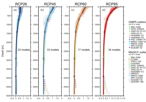
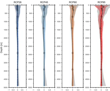
The MAGICC ocean model update yields optimal parame-ter sets for every CMIP5 model used in the calibration pro-cedure outlined above. Those sets are listed in Table 1. In Fig. 2, we show both the 90 % model range and the me-dian for the reference CMIP5 global potential ocean tem-perature anomalies as well as the median MAGICC global ocean warming profile averaged over 2081 to 2100 relative to the reference period 1986 to 2005. The figure also provides information on individual model outliers for reference data and calibration results. Corresponding potential ocean tem-perature residuals are shown in Fig. A1. MAGICC is able to capture the key CMIP5 features for all RCP scenarios. The median model response either matches or is close to the
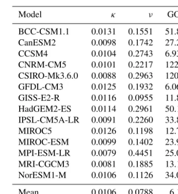
me-Table 2.Glacier sea level component calibration results with pa-rameter sets for the available CMIP5 models. Calibration parame-ters are introduced in Sect. 2.6. GOF is given as weighted RSS di-vided by the number of calibrated model years (weight glacier SLE contribution [mm]: 1). The optimal set for the mean response of the calibration data is given at the bottom of the table.
Model κ ν GOF
BCC-CSM1.1 0.0131 0.1551 51.88
CanESM2 0.0098 0.1742 27.22
CCSM4 0.0104 0.2743 6.935
CNRM-CM5 0.0101 0.2217 122.8
CSIRO-Mk3.6.0 0.0088 0.2963 120.1
GFDL-CM3 0.0125 0.1932 6.061
GISS-E2-R 0.0116 0.0955 11.81
HadGEM2-ES 0.0114 0.2961 50.19
IPSL-CM5A-LR 0.0091 0.2260 33.82
MIROC5 0.0126 0.1198 12.77
MIROC-ESM 0.0099 0.1402 23.91
MPI-ESM-LR 0.0079 0.4451 25.04
MRI-CGCM3 0.0081 0.1885 13.10
NorESM1-M 0.0106 0.1126 34.04
Mean 0.0106 0.0788 6.10
dian of the CMIP5 responses. The updated MAGICC ocean deviates from the CMIP5 data in a few cases. Generally, there appears to be less warming in the mid-ocean between around 1500 m and 2500 m than in the CMIP5 reference data. Also, there is a tendency for the MAGICC bottom layers to warm more than the CMIP5 reference data. However, it is only for two of the 36 CMIP5 models used that calibration re-sults show a major bottom layer warming bias. The GISS-E2-R reference data show strong mid-layer warming com-bined with actual bottom layer cooling, while the HadGEM2-CC data show cooling in the upper 500 m over the histori-cal period (see Fig. A2). In both cases, the MAGICC hemi-spheric upwelling-diffusion ocean model cannot fully cap-ture these characteristics. For the HadGEM2-CC emulation, MAGICC overcompensates the surface cooling with strong bottom layer warming. Apart from these anomalies, the cali-brated MAGICC ocean component captures the hemispheri-cally averaged CMIP5 ocean warming for the different RCP scenarios well (Figs. 2 and A1). We derive CMIP5-consistent thermal expansion estimates based on the optimal ocean rameter sets and the additional thermal expansion scaling pa-rameterφ(see Table 1).
ex-−0.5 0 0.5 1 1.5 2 0
500
1000
1500
2000
2500
3000
3500
4000
4500
5000
Temperature change [K]
Depth [m]
RCP26
23 models
−0.5 0 0.5 1 1.5 2 0
500
1000
1500
2000
2500
3000
3500
4000
4500
5000
−0.5 0 0.5 1 1.5 2 0
500
1000
1500
2000
2500
3000
3500
4000
4500
5000
RCP60
17 models
−0.5 0 0.5 1 1.5 2 2.5 3 3.5 0
500
1000
1500
2000
2500
3000
3500
4000
4500
5000
(a) (b) (c) (d)
GFDL−ESM2G
MIROC−ESM
RCP45
33 models
NorESM1−M NorESM1−ME
RCP85
34 models
GFDL−ESM2G
GISS−E2−R HadGEM2−CC
IPSL−CM5B−LR MIROC−ESM−CHEM MIROC−ESM MRI−CGCM3 NorESM1−M
BNU−ESM CCSM4
CanESM2
GISS−E2−R−CC GISS−E2−R HadGEM2−CC MIROC5
MRI−CGCM3 CMIP5 outliers: (wrt 90 % range)
MAGICC outliers: (wrt 90 % range)
BNU−ESM
GISS−E2−R−CC
HadGEM2−ES
CMCC−CM
Figure 2.Potential ocean temperature depth profiles for MAGICC and reference CMIP5 warming under RCP2.6, RCP4.5, RCP6.0, and RCP8.5 scenarios, 2081–2100 anomalies with respect to 1986–2005. Interpolated CMIP5 90 % model ranges and corresponding median profiles are shown in colors, with circles indicating the individual MAGICC ocean layers. MAGICC median ocean-warming profiles given as black lines with open circles indicating selected layers for ocean calibration. Model outliers not covered by the respective 90 % ranges are shown for both CMIP5 reference data and MAGICC calibration results. Potential ocean temperature residuals of the calibration are provided for every MAGICC ocean layer in Fig. A1.
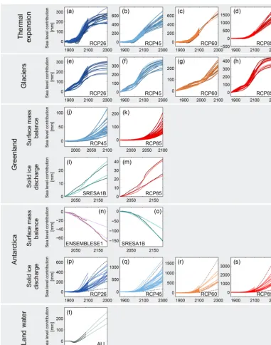
pansion time series. Relative to 1850, the calibration yields a 2100 thermosteric SLR range of 104 to 238 mm (CMIP5: 113 to 231 mm) for RCP2.6, 151 to 307 mm (161 to 290 mm) for RCP4.5, 166 to 331 mm (174 to 309 mm) for RCP6.0, and 219 to 491 mm (261 to 445 mm) for RCP8.5. The cor-responding 1850 to 2300 thermosteric SLR responses range from 192 to 335 mm for RCP2.6 (CMIP5: 180 to 288 mm), 348 to 709 mm for RCP4.5 (345 to 707 mm), 586 to 717 mm for RCP6.0 (635 to 658 mm), and 1040 to 1794 mm for RCP8.5 (1040 to 1909 mm). In contrast to some detrended
zostogaCMIP5 model time series, the MAGICC thermal ex-pansion projections do not show negative slopes in the 20th century, which is consistent with observations (Church et al., 2013b).
The calibrated global glacier SLR response and the cor-responding reference data are shown in panels (e) to (h), while the specific calibration results are listed in Table 2. The MAGICC projections show good agreement with the updated Marzeion et al. (2012) data (Fig. 3e to h). Relative to 1850,
the estimated glacier SLE contributions in 2100 are 145 to 259 mm (Marzeion et al., 2014: 134 to 256 mm) for RCP2.6, 162 to 276 mm (159 to 277 mm) for RCP4.5, 163 to 276 (163 to 276 mm) for RCP6.0, and 188 to 302 mm (198 to 308 mm) for RCP8.5. For 2300, projected SLR from glaciers amounts to a SLE range of 177 to 298 mm (Marzeion et al., 2014: 188 to 305 mm) for RCP2.6, 255 to 374 mm (254 to 366 mm) for RCP4.5, and 325 to 439 mm (338 to 444 mm) for RCP8.5.
cali-Figure 3.MAGICC sea level model calibration results for thermal expansion(a–d), global glaciers(e–h), Greenland surface mass balance(j– k)and solid ice discharge(l–m), Antarctic surface mass balance(n–o), and solid ice discharge(p–s), as well as land water(t). The panels show scenario-specific calibrated MAGICC sea level responses as colored lines, with underlying reference data as thin dark lines. Antarctic solid ice discharge reference 90 % range plus corresponding median are provided as thin dashed lines. Climate-independent land water projections are identical to the reference data until 2100 (see Sect. 2.5). Please note thatxandyaxis ranges differ for individual panels.
bration results listed in Table 4. As presented by Nick et al. (2013), we show projections of the minimum and maximum cases for the combined contribution from the four major out-let glaciers prior to up-scaling to the entire Greenland ice sheet. Estimates are provided relative to the year 2000. For the SRES A1B scenario, the SLE projections range from 17 to 28 mm (Nick et al., 2013: 14 to 25 mm) for the last year
of the available reference data in 2190. For the same year, we project 24 to 42 mm (26 to 43 mm) based on the RCP8.5 scenario.
Table 3.Greenland SMB sea level component calibration results with optimal parameter sets for the available CMIP5 models. Cal-ibration parameters are introduced in Sect. 2.6. GOF is given as weighted RSS divided by the number of calibrated model years (weight Greenland SMB SLE contribution [mm]: 1). The optimal set for the mean response of the calibration data is given at the bot-tom of the table.
Model υ χ ϕ GOF
ACCESS1.0 0.2190 0.9748 3.2749 0.74
ACCESS1.3 0.2021 0.2490 1.2781 0.46
BCC-CSM1.1 0.0664 0.2398 2.3731 0.56
BNU-ESM 0.1290 0.0000 1.9068 0.89
CanESM2 0.0656 0.0000 2.2971 1.96
CCSM4 0.0186 0.0000 2.7122 1.17
CESM1-BGC 0.0618 0.0000 1.9517 1.06
CMCC-CM 0.0830 0.0000 1.9688 1.57
CNRM-CM5 0.1009 0.0000 1.8283 0.36
CSIRO-Mk3.6.0 0.1459 0.4702 1.8740 0.60
GFDL-CM3 0.3347 0.7326 2.2962 0.56
GFDL-ESM2M 0.1077 0.0000 2.0794 0.90
GISS-E2-R 0.1302 0.0000 1.9605 0.26
HadGEM2-CC 0.2308 0.9594 2.9988 0.27
HadGEM2-ES 0.1974 0.8354 2.2872 0.55
IPSL-CM5A-LR 0.1762 0.4514 1.8847 0.25
IPSL-CM5A-MR 0.0802 0.0000 2.0480 0.67
IPSL-CM5B-LR 0.0531 0.0000 2.4263 0.99
MIROC5 0.2168 0.0000 1.8440 1.11
MIROC-ESM-CHEM 0.1557 0.3454 2.1621 1.51
MIROC-ESM 0.1549 0.5188 2.3107 1.10
MPI-ESM-LR 0.0333 0.0000 2.6372 1.49
MRI-CGCM3 0.0645 0.0000 2.2958 0.59
NorESM1-M 0.0969 0.0000 2.0000 0.50
Mean 0.1148 0.0000 2.0169 0.47
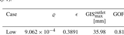
Table 4. Greenland SID sea level component calibration results with optimal parameter sets for the low and high cases introduced by Nick et al. (2013). Calibration parameters are introduced in Sect. 2.6. GOF is given as weighted RSS divided by the number of calibrated model years (weight Greenland SID SLE contribution [mm]: 1).
Case % GISoutletmax GOF
[mm]
Low 9.062×10⁻⁴ 0.3891 35.98 0.81
High 7.933×10⁻⁴ 0.4722 53.63 1.62
(2013) provides projections that go beyond 2100 only for the model HadCM3. For the ENSEMBLES E1 scenario, the two model-specific 2100 SLE responses range from −29 to−18 mm (Ligtenberg et al., 2013:−27 to−20 mm). The 2200 estimate lies at−67 mm (−73 mm) based on the HadCM3 parameter set. The 2100 values for the SRES A1B scenario span from−51 to−33 mm (Ligtenberg et al., 2013: −44 to −32 mm), while the 2200 Antarctic SMB SLE
re-Table 5. Antarctic SMB sea level component calibration results with optimal parameter sets for the CMIP3 models ECHAM5 and HadCM3. Calibration parameters are introduced in Sect. 2.6. GOF is given as weighted RSS divided by the number of calibrated model years (weight Antarctic SMB SLE contribution [mm]: 1). The opti-mal set for the mean response of the calibration data is given at the bottom of the table.
Model ξ ρ σ GOF
ECHAM5 −0.11028 0.0000 1.2435 0.70
HadCM3 −0.13869 0.0000 1.3910 9.61
Mean −0.12082 0.0000 1.5234 0.70
sponse is projected to be −158 mm (−163 mm). As we model the Antarctic SID sea level component with the linear response function approach presented by Levermann et al. (2014), it is not calibrated against any reference data. The MAGICC component utilizes the responses from the three ice-sheet models of that study, which include an explicit rep-resentation of ice-shelf dynamics. As the sea level responses for this subset of ice-shelf models are not available, we show the 90 % model range and the median of all five ice-sheet models from Levermann et al. (2014) in Fig. 3p to s. CMIP5 model-specific parameter sets have been determined for the three different ice-shelf models (Levermann et al., 2014, Ta-bles 2–5). For 1850 to 2100, the 90 % ranges of the MAGICC responses based on the ice-shelf model subset correspond to 33 to 253 mm SLE (Levermann et al., 2014: 15 to 227 mm) for RCP2.6, 39 to 319 mm (17 to 267 mm) for RCP4.5, 42 to 338 mm (17 to 277 mm) for RCP6.0, and 53 to 448 mm (20 to 365 mm) for RCP8.5. For 1850 to 2300, 90 % of the MAGICC projections lie within 115 and 874 mm SLE (Lev-ermann et al., 2014: 69 to 635 mm) for RCP2.6, 209 and 1435 mm (119 to 1182 mm) for RCP4.5, 282 and 1860 mm (161 to 1719 mm) for RCP6.0, and 505 and 3173 mm (300 to 3535 mm) for RCP8.5, respectively. The MAGICC Antarctic SID estimates, which are based on the physically more com-plex ice-shelf models only, mostly lie within the 90 % range of Antarctic SID sea level contributions provided by Lever-mann et al. (2014).
In panel (t), we show SLE responses for the scenario-independent land water SLE component. From 1900 to 2100, we include the net land water SLE contribution as presented in Fig. 3 of Wada et al. (2012), corrected by the 20 % frac-tion of land water that does not reach the global ocean Wada et al. (2016). Post-2100, we assume a constant annual con-tribution based on the assumptions outlined in Sect. 2.5. 2100 estimates span a global sea level contribution of 39 to 77 mm. The extended land water projections range from 156 to 261 mm SLE for 2300.
different MAGICC setups are used to project global SLR un-til 2100 and 2300 based on the four RCP scenarios and their extensions. The ocean model update is not sufficient to make the MAGICC model fully CMIP5 consistent because other crucial climate system components such as the carbon cy-cle have not been updated yet. To overcome this issue, we constrain the MAGICC model with available CMIP5 global-mean tastime series. Together with the corresponding cali-brated MAGICC ocean model parameter sets, we are able to create a CMIP5 environment that allows us to compare our 2100 global SLR projections to the latest IPCC estimates. Beyond 2100, the number of available CMIP5 simulations is much smaller, with only two 2300 model runs available for RCP6.0, for example. In order to also provide a sufficiently large number of model runs for 2300, we use 600 histori-cally constrained parameter sets that have been derived us-ing a probabilistic Metropolis–Hastus-ings Markov chain Monte Carlo method (Meinshausen et al., 2009). This approach has been extended to also reflect carbon-cycle uncertainties (Friedlingstein et al., 2014) and the climate sensitivity range of the latest IPCC assessment (Flato et al., 2013; Rogelj et al., 2012, 2014). For this second setup, MAGICC is not forced to match CMIP5 global-meantas, allowing us to provide con-sistent ensemble projections out to 2300. For this ensemble, we randomly draw from the CMIP5 ocean model parame-ter sets and the calibration results for each sea level model component. Random samples are also sourced between the minimum and maximum realizations for the Greenland SID and LWS component as well as between the empirical basal melt sensitivities for the Antarctic SID contribution (Lever-mann et al., 2014). For consistency, we adopt the same en-semble size for the CMIP5 constrained MAGICC setup and randomly select the specific CMIP5 global-meantastime se-ries in addition to the other randomized parameter sets from the individual sea level components.
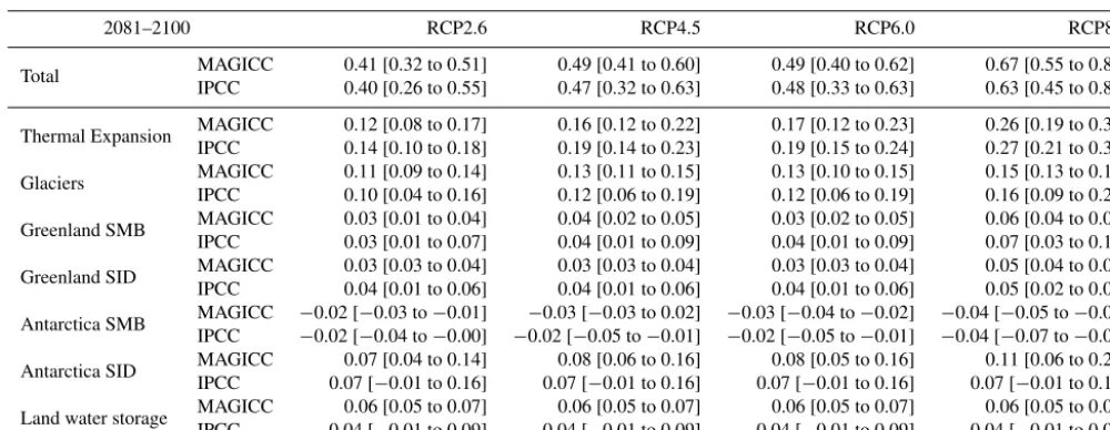
In Table 6, we show median SLR estimates for the 2081– 2100 average relative to 1986–2005 and 66 % ranges for every individual component, with corresponding IPCC ref-erence estimates and likely ranges. The individual MAG-ICC sea level contributions are in good agreement with the IPCC estimates. Figure 4 shows the full suite of MAG-ICC SLR projections for the RCP scenarios. The smaller panels (a) to (d) give 90 and 66 % ranges as well as me-dian responses for all RCP scenarios until 2100 based on the CMIP5-consistent setup. Additional bars are provided for the IPCC reference data and the probabilistic MAGICC setup, which is not constrained to CMIP5. For the CMIP5-consistent MAGICC setup, 2100 median SLR is projected to be 0.45 m (66 % range: 0.35 m to 0.56 m) for RCP2.6, 0.55 m (0.45 to 0.67 m) for RCP4.5, 0.56 m for (0.46 to 0.71 m) for RCP6.0, and 0.79 m (0.65 to 0.97 m) for RCP8.5 (see also Table 7). All SLR projections are provided relative to the reference period 1986 to 2005. MAGICC SLR estimates for 2100 are generally higher than the IPCC projections. CMIP5-consistent projections of average 2081 to 2100 SLR lie well
within the IPCC range, with median estimates on average 0.02 m higher than the corresponding IPCC values (Church et al., 2013a). In panel (e), we provide 2300 SLR projections for the RCP extensions based on the probabilistic MAGICC setup, which is not constrained to CMIP5. For RCP2.6, the median SLR response is 1.02 m (66 % range: 0.80 to 1.35 m). We project a median of 1.76 m (1.29 to 2.30 m) for RCP4.5, 2.38 m (1.72 to 3.20 m) for RCP6.0, and up to 4.73 m (3.41 to 6.82 m) for RCP8.5 (see also Table 7). In Fig. A3, we pro-vide MAGICC SLR hindcast results and three comparison datasets for the period 1900 to 2000. The MAGICC sea level model shows good agreement with the observational datasets based on Church et al. (2011) and Hay et al. (2015). The global 1900–2300 SLR responses are provided for all RCPs and each sea level component in the Appendix Figs. A4 to A7.
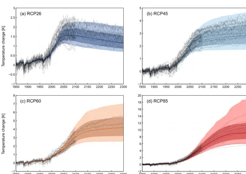
Figure 5 shows the global-mean tas responses based on the historically constrained, probabilistic MAGICC setup, which is used for the 2300 SLR projections. Each panel also includes the available CMIP5 global-mean tas time series; 2300 MAGICC median global-meantasfall well within the available CMIP5 range for RCP4.5, RCP6.0, and RCP8.5. The MAGICC median global-mean tas response is at the lower end of 2300 CMIP5 temperatures for RCP2.6. For this scenario, the projected cooling over 22nd and 23rd cen-turies is consistent with previous MAGICC studies, e.g., Meinshausen et al. (2011c). The overall historically con-strained, probabilistic MAGICC global-mean tas response for the 21st century is stronger than in the CMIP5 refer-ence data for RCP4.5, RCP6.0, and RCP8.5 scenarios. This slightly steeper 21st century global-mean tas slope is also reflected in the corresponding probabilistic MAGICC 2100 SLR estimates, given the strong air temperature dependence of the sea level model (see Fig. 4a to d).
4 Discussion
Table 6.The 2081–2100 median values and 66 % ranges for global SLR projections relative to 1986–2005 in meters, resolved by sea level components for the four RCP scenarios. Estimates are provided based on the CMIP5-consistent MAGICC setup. IPCC median projections and likely ranges are given as a reference.
2081–2100 RCP2.6 RCP4.5 RCP6.0 RCP8.5
Total MAGICC 0.41 [0.32 to 0.51] 0.49 [0.41 to 0.60] 0.49 [0.40 to 0.62] 0.67 [0.55 to 0.83] IPCC 0.40 [0.26 to 0.55] 0.47 [0.32 to 0.63] 0.48 [0.33 to 0.63] 0.63 [0.45 to 0.82]
Thermal Expansion MAGICC 0.12 [0.08 to 0.17] 0.16 [0.12 to 0.22] 0.17 [0.12 to 0.23] 0.26 [0.19 to 0.34] IPCC 0.14 [0.10 to 0.18] 0.19 [0.14 to 0.23] 0.19 [0.15 to 0.24] 0.27 [0.21 to 0.33]
Glaciers MAGICC 0.11 [0.09 to 0.14] 0.13 [0.11 to 0.15] 0.13 [0.10 to 0.15] 0.15 [0.13 to 0.17] IPCC 0.10 [0.04 to 0.16] 0.12 [0.06 to 0.19] 0.12 [0.06 to 0.19] 0.16 [0.09 to 0.23]
Greenland SMB MAGICC 0.03 [0.01 to 0.04] 0.04 [0.02 to 0.05] 0.03 [0.02 to 0.05] 0.06 [0.04 to 0.09] IPCC 0.03 [0.01 to 0.07] 0.04 [0.01 to 0.09] 0.04 [0.01 to 0.09] 0.07 [0.03 to 0.16]
Greenland SID MAGICC 0.03 [0.03 to 0.04] 0.03 [0.03 to 0.04] 0.03 [0.03 to 0.04] 0.05 [0.04 to 0.06] IPCC 0.04 [0.01 to 0.06] 0.04 [0.01 to 0.06] 0.04 [0.01 to 0.06] 0.05 [0.02 to 0.07]
Antarctica SMB MAGICC −0.02 [−0.03 to−0.01] −0.03 [−0.03 to 0.02] −0.03 [−0.04 to−0.02] −0.04 [−0.05 to−0.03] IPCC −0.02 [−0.04 to−0.00] −0.02 [−0.05 to−0.01] −0.02 [−0.05 to−0.01] −0.04 [−0.07 to−0.01]
Antarctica SID MAGICC 0.07 [0.04 to 0.14] 0.08 [0.06 to 0.16] 0.08 [0.05 to 0.16] 0.11 [0.06 to 0.21] IPCC 0.07 [−0.01 to 0.16] 0.07 [−0.01 to 0.16] 0.07 [−0.01 to 0.16] 0.07 [−0.01 to 0.16]
Land water storage MAGICC 0.06 [0.05 to 0.07] 0.06 [0.05 to 0.07] 0.06 [0.05 to 0.07] 0.06 [0.05 to 0.07] IPCC 0.04 [−0.01 to 0.09] 0.04 [−0.01 to 0.09] 0.04 [−0.01 to 0.09] 0.04 [−0.01 to 0.09]
Sea le
vel r
ise [m]
Sea le
vel r
ise [m]
IPCC
Year
MA
GICC CMIP5
MA
GICC PR
OB
Sea le
vel r
ise [m]
20000 2020 2040 2060 2080 2100 0.2
0.4 0.6 0.8 1.0 1.2
20000 2020 2040 2060 2080 2100 0.2
0.4 0.6 0.8 1.0 1.2
20000 2020 2040 2060 2080 2100 0.2
0.4 0.6 0.8 1.0 1.2
20000 2020 2040 2060 2080 2100 0.2
0.4 0.6 0.8 1.0 1.2
20000 2050 2100 2150 2200 2250 2300 1.0
2.0 3.0 4.0 5.0 6.0 7.0
(a) RCP26 (b) RCP45
(c) RCP60 (d) RCP85
(e) ALL RCPs
Table 7.The 2100 and 2300 median values as well as 66 % ranges for total global SLR projections relative to 1986–2005 based on the MAGICC CMIP5 and MAGICC PROB experimental designs. IPCC median projections and likely ranges are given as a reference.
2100 2300
RCP2.6
MAGICC CMIP5 0.45 [0.35 to 0.56] –
MAGICC PROB 0.48 [0.37 to 0.59] 1.02 [0.80 to 1.35]
IPCC 0.44 [0.28 to 0.61] –
RCP4.5
MAGICC CMIP5 0.55 [0.45 to 0.67] –
MAGICC PROB 0.61 [0.48 to 0.74] 1.76 [1.29 to 2.30]
IPCC 0.53 [0.36 to 0.71] –
RCP6.0
MAGICC CMIP5 0.56 [0.46 to 0.71] –
MAGICC PROB 0.65 [0.52 to 0.79] 2.38 [1.72 to 3.20]
IPCC 0.55 [0.38 to 0.73] –
RCP8.5
MAGICC CMIP5 0.79 [0.65 to 0.97] –
MAGICC PROB 0.89 [0.68 to 1.09] 4.73 [3.41 to 6.82]
IPCC 0.74 [0.52 to 0.98] –
1850 1900 1950 2000 2050 2100 2150 2200 2250 2300 −1
−0.5 0 0.5 1 1.5 2 2.5 3
1850 1900 1950 2000 2050 2100 2150 2200 2250 2300 −1
0 1 2 3 4 5
1850 1900 1950 2000 2050 2100 2150 2200 2250 2300 −1
0 1 2 3 4 5 6 7 8
1850 1900 1950 2000 2050 2100 2150 2200 2250 2300 −2
0 2 4 6 8 10 12 14 16 18 20
(a) RCP26 (b) RCP45
(c) RCP60 (d) RCP85
Year Year
Temper
ature change [K]
Temper
ature change [K]
based on Marzeion et al. (2014). The SMB and SID pa-rameterizations for both ice sheets reflect available process-based reference data (Fettweis et al., 2013; Nick et al., 2013; Ligtenberg et al., 2013; Levermann et al., 2014). In addition, new process understanding has been included in the land wa-ter component (Wada et al., 2016). The full MAGICC model, including the sea level module, can be run in less than 1 s for 100 model years on a single core. This makes it an efficient platform to provide large ensembles of global sea level pro-jections.
Projecting SLR beyond 2100 and providing physically consistent global estimates out to 2300 has been one of the key motivations for the development of the MAGICC sea level model. For five of the seven sea level components, the reference data used for calibrating the individual contribu-tions extend beyond 2100. For thermal expansion, global glacier, and Antarctic SID contributions, the reference cal-ibration period spans from 1850 to 2300. The remaining components are based on physically plausible assumptions, which allow us to also provide 2300 estimates, assuming that the calibrated parameterizations for each sea level compo-nent remain valid. Our sea level model transparently em-ulates and combines long-term sea level projections from process-based models. It is also in line with observed past total sea level change (see Fig. A3). The close reproduction of selected reference data (Figs. 3 and A3), together with the consistent translation of climate forcing into a SLR re-sponse within the MAGICC model, and the comprehensive representation of relevant processes (e.g., the thermal expan-sion contribution produced by the CMIP5-consistent MAG-ICC ocean model and the inclusion of the land water storage sea level component) make the MAGICC sea level model a powerful addition to the existing sea level emulators.
Both CMIP5 ocean and air temperatures serve as input for the presented sea level model. Other published sea level emu-lators only utilize air temperature projections, also provided by MAGICC, either based purely on available CMIP3 cal-ibration results (Meinshausen et al., 2011a; Perrette et al., 2013) or an updated historically constrained probabilistic MAGICC setup that reflects the latest IPCC climate sensitiv-ity estimates (Schleussner et al., 2016; Mengel et al., 2016). We here provide the first major step to making MAGICC fully CMIP5 consistent, with the ocean model now emulating 36 CMIP5 hemispheric potential ocean temperature and ther-mal expansion responses. However, other crucial elements of the MAGICC model, like the atmosphere and the car-bon cycle, are not yet calibrated to CMIP5. When combining the CMIP5-calibrated ocean with the older atmosphere and carbon-cycle calibrations, the resulting 21st century warm-ing is slightly stronger than CMIP5 (see Fig. 5). To ensure a robust MAGICC sea level model, the individual compo-nents were either calibrated with prescribed CMIP5 temper-atures, or with CMIP3-consistent time series whenever the reference data was based on the older generation of SRES and ENSEMBLES scenarios. The quality of the sea level
model calibration is therefore not affected by the warmer MAGICC air temperature response. Our primary 2100 SLR projections are based on a MAGICC ensemble that is con-strained by CMIP5 global-meantas. These projections can therefore be directly compared to recent IPCC estimates. For our 2300 projections, we run MAGICC in the historically constrained, probabilistic setup described above. The result-ing MAGICC air temperature responses mostly reflect the available CMIP5 reference data, although they show a shorter response time scale (see Fig. 5). These differences to CMIP5 translate into the corresponding SLR projections due to the strong air temperature dependence of the sea level model. Hence, the MAGICC sea level module will only be able to provide fully CMIP5-consistent SLR responses for 2300 once the remaining components of the MAGICC model have been updated.
only yield up to around 0.35 m in 2100 and 2.68 m in 2300 for the upper bound of the 90 % range. As the more recent research suggests, these estimates may be too low, indicat-ing that the Antarctic contribution to future SLR is subject to additional uncertainties. This illustrates the need to han-dle long-term SLR projections with care and to note the cor-responding methodological caveats; in particular, those sur-rounding the representation of Antarctic ice-sheet changes.
The MAGICC sea level model assesses long-term global SLR trajectories by synthesizing available process-based projections for the individual sea level drivers and apply-ing them to the available set of RCP scenarios and their ex-tensions until 2300. The current version shows 2100 esti-mates that are well within the range of the latest IPCC as-sessment (see Fig. 4). The structure of the emulator makes the MAGICC sea level model a computationally much more efficient tool compared to the comprehensive and complex process-based models. The calibration routines for the in-dividual components have been flexibly designed to allow for timely updates whenever new robust modeling results
be-come available. The presented MAGICC sea level model, to-gether with the MAGICC ocean model update, are new el-ements of MAGICC model version 6 (Meinshausen et al., 2011a). The implementation of the new sea level model ini-tiates the development of MAGICC model version 7 to com-prehensively emulate CMIP5 projections. The full potential of the MAGICC sea level model will be unlocked once this MAGICC model upgrade has been completed.
Appendix A
Additional information on MAGICC sea level model calibra-tion parameters, MAGICC ocean model calibracalibra-tion results, MAGICC SLR hindcast quality, and component-wise MAG-ICC SLR projections for 1900–2300.
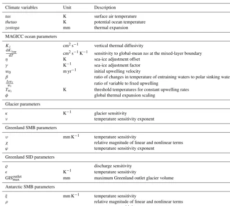
Table A1.List of variables and free parameters used for the individual MAGICC sea level component calibrations.
Climate variables Unit Description
tas K surface air temperature
thetao K potential ocean temperature
zostoga mm thermal expansion
MAGICC ocean parameters
Kz cm2s−1 vertical thermal diffusivity
dKztop
dT cm
2s−1K−1 sensitivity to global-meantasat the mixed-layer boundary
η K sea-ice adjustment offset
γ K−1 sea-ice adjustment factor
w0 m yr−1 initial upwelling velocity
β ratio of changes in temperature of entraining waters to polar sinking waters
1wt
wt ratio of variable to fixed upwelling
Twt K threshold temperatures for constant upwelling rates
φ global thermal expansion scaling
Glacier parameters
κ K−1 glacier sensitivity
ν temperature sensitivity exponent
Greenland SMB parameters
υ mm K−1 temperature sensitivity
χ relative magnitude of linear and nonlinear terms
ϕ temperature sensitivity exponent
Greenland SID parameters
% discharge sensitivity
K−1 temperature sensitivity
GISoutletmax mm maximum Greenland outlet glacier volume
Antarctic SMB parameters
ξ mm K−1 temperature sensitivity
ρ relative magnitude of linear and nonlinear terms
−1 −0.5 0 0.5 1 0
500
1000
1500
2000
2500
3000
3500
4000
4500
5000
−0.5 0 0.5 1 0
500
1000
1500
2000
2500
3000
3500
4000
4500
5000
−1 −0.5 0 0.5 1 0
500
1000
1500
2000
2500
3000
3500
4000
4500
5000
−1 −0.5 0 0.5 1 0
500
1000
1500
2000
2500
3000
3500
4000
4500
5000 −1
Temperature change [K]
Depth [m]
RCP26 RCP45 RCP60 RCP85
−0.5 0 0.5 1 1.5 2 5000
4500 4000 3500 3000 2500 2000 1500 1000 500
0 HadGEM2-CC
Depth [m]
Temperature change [K]
−0.5 0 0.5 1 1.5 2
5000 4500 4000 3500 3000 2500 2000 1500 1000 500
0 GISS-E2-R
−1 0 1 2 3
5000 4500 4000 3500 3000 2500 2000 1500 1000 500
0 CCSM4
Figure A2.Annual RCP4.5 ocean warming anomalies for the CMIP5 models GISS-E2-R (1850–2300), HadGEM2-CC (1850–2100), and CCSM (1850–2300), relative to 1850 and globally averaged. Annual potential ocean temperature anomaly profiles are shown as dark blue in 1850 via green and yellow to red for the last year of the reference data.
1900 1910 1920 1930 1940 1950 1960 1970 1980 1990 2000 −180
−160 −140 −120 −100 −80 −60 −40 −20 0
MAGICC sea level model Mengel et al. (2016) Hay et al. (2015)
updated Church et al. (2011)
Year
Sea le
vel r
ise wr
t 1986–2005 [mm]
1900 2000 2100 2200 2300 0
0.5 1 1.5 2 2.5
1900 2000 2100 2200 2300
0 300 600 900 1200 1500
1900 2000 2100 2200 2300
0 100 200 300 400 500 600 700
1900 2000 2100 2200 2300
0 30 60 90 120 150
1900 2000 2100 2200 2300
−20 0 20 40 60 80 100
1900 2000 2100 2200 2300
−50 0 50 100 150 200
1900 2000 2100 2200 2300
−100 −80 −60 −40 −20 0
1900 2000 2100 2200 2300
0 100 200 300 400 500
1900 2000 2100 2200 2300
0 50 100 150 200 250
Sea le
vel r
ise [mm]
(a) GMT (b) Total SLR
Temper
ature change [K]
(c) THEXP
(f) GL (e) GIS SID
(d) GIS SMB
(g) AIS SMB (h) AIS SID (i) LW
Sea le
vel r
ise [mm]
Sea le
vel r
ise [mm]
Sea le
vel r
ise [mm]
Sea le
vel r
ise [mm]
Sea le
vel r
ise [mm]
Sea le
vel r
ise [mm]
Sea le
vel r
ise [mm]
Year
1900 2000 2100 2200 2300 0
1 2 3 4
1900 2000 2100 2200 2300
0 500 1000 1500 2000 2500
1900 2000 2100 2200 2300
0 200 400 600 800 1000 1200 1400
1900 2000 2100 2200 2300
0 100 200 300 400
1900 2000 2100 2200 2300
0 30 60 90 120 150
1900 2000 2100 2200 2300
−50 0 50 100 150 200 250
1900 2000 2100 2200 2300
−200 −150 −100 −50 0
1900 2000 2100 2200 2300
0 200 400 600 800 1000
1900 2000 2100 2200 2300
0 50 100 150 200 250
Sea le
vel r
ise [mm]
(a) GMT (b) Total SLR
Temper
ature change [K]
(c) THEXP
(f) GL (e) GIS SID
(d) GIS SMB
(g) AIS SMB (h) AIS SID (i) LW
Sea le
vel r
ise [mm]
Sea le
vel r
ise [mm]
Sea le
vel r
ise [mm]
Sea le
vel r
ise [mm]
Sea le
vel r
ise [mm]
Sea le
vel r
ise [mm]
Sea le
vel r
ise [mm]
Year