www.geosci-model-dev.net/9/947/2016/ doi:10.5194/gmd-9-947-2016
© Author(s) 2016. CC Attribution 3.0 License.
Couplerlib: a metadata-driven library for the integration of multiple
models of higher and lower trophic level marine systems with
inexact functional group matching
Jonathan Beecham1, Jorn Bruggeman2, John Aldridge1, and Steven Mackinson1
1Cefas Lowestoft Laboratory, Pakefield Road, Lowestoft, Suffolk, NR33 0HT, UK 2Bolding & Burchard ApS. Strandgyden 25, 5466 Asperup, Denmark
Correspondence to: Jonathan Beecham ([email protected])
Received: 31 March 2015 – Published in Geosci. Model Dev. Discuss.: 20 July 2015 Revised: 29 January 2016 – Accepted: 6 February 2016 – Published: 4 March 2016
Abstract. End-to-end modelling is a rapidly developing strategy for modelling in marine systems science and man-agement. However, problems remain in the area of data matching and sub-model compatibility. A mechanism and novel interfacing system (Couplerlib) is presented whereby a physical–biogeochemical model (General Ocean Turbulence Model–European Regional Seas Ecosystem Model, GOTM– ERSEM) that predicts dynamics of the lower trophic level (LTL) organisms in marine ecosystems is coupled to a dy-namic ecosystem model (Ecosim), which predicts food-web interactions among higher trophic level (HTL) organisms. Coupling is achieved by means of a bespoke interface, which handles the system incompatibilities between the models and a more generic Couplerlib library, which uses metadata de-scriptions in extensible mark-up language (XML) to marshal data between groups, paying attention to functional group mappings and compatibility of units between models. In ad-dition, within Couplerlib, models can be coupled across net-works by means of socket mechanisms.
As a demonstration of this approach, a food-web model (Ecopath with Ecosim, EwE) and a physical–biogeochemical model (GOTM–ERSEM) representing the North Sea ecosys-tem were joined with Couplerlib. The output from GOTM– ERSEM varies between years, depending on oceanographic and meteorological conditions. Although inter-annual vari-ability was clearly present, there was always the tendency for an annual cycle consisting of a peak of diatoms in spring, followed by (less nutritious) flagellates and dinoflagellates through the summer, resulting in an early summer peak in the mesozooplankton biomass. Pelagic productivity, predicted
by the LTL model, was highly seasonal with little winter food for the higher trophic levels. The Ecosim model was orig-inally based on the assumption of constant annual inputs of energy and, consequently, when coupled, pelagic species suf-fered population losses over the winter months. By contrast, benthic populations were more stable (although the benthic linkage modelled was purely at the detritus level, so this sta-bility reflects the stasta-bility of the Ecosim model). The coupled model was used to examine long-term effects of environmen-tal change, and showed the system to be nutrient limited and relatively unaffected by forecast climate change, especially in the benthos. The stability of an Ecosim formulation for large higher tropic level food webs is discussed and it is con-cluded that this kind of coupled model formulation is better for examining the effects of long-term environmental change than short-term perturbations.
1 Introduction
international projects such as MEECE (Marine Ecosystem Evolution in a Changing Environment; www.meece.eu) have been set up to produce integrative modelling systems in order to assess the likely impact of anthropogenic change. How-ever, the problem which remains is that the models that are used in an end-to-end modelling system are themselves com-plicated with many parameters. Joining such models end to end has been described as “putting lipstick on a pig” (Rose, 2012), and an appeal is sometimes made to start with simpler models (Fulton et al., 2003).
Given the choice between constructing end-to-end model systems de novo and joining existing models (usually written by different teams, often in different languages or even run-ning on separate machines) together “Frankenstein style” or even combining multiple models at source level, the former has a number of obvious advantages. The multiple models (or multiple components of an integrated modelling system) can benefit from a unified design process, can use a consistent co-ordinate system and model entity representation, and can benefit from unified data input, output, visualization, control, and validation. Most importantly, the models can be aligned in terms of whether they are strategic models for explor-ing general principles, or tactical models designed to explore specific aspects of the system with a high degree of detail and domain-specific knowledge (Levins, 1966). Joining models with widely differing focus will typically result in a com-bined model with only broad results for a narrow domain, and yet will still require a large amount of data to calibrate it. On the other hand, we are often forced to work with com-bining existing models because of the existence of code, with updates and a user community, the investment of time in the lengthy processes of calibrating, and validating these mod-els. Combining models by formally combining code can im-prove the reliability and intelligibility of the model and make validation easier, but combines the disadvantage of unsympa-thetic algorithms having to work together with an inability to easily incorporate code updates to the original sources. For most modelling projects, sociological aspects of the mod-elling process will have an influence on the strategy of the end-to-end modelling employed.
In many cases the objective of the end-to-end modelling approach includes a high degree of prediction, for example, it is one of the aims of the EU Framework programme 7 project MEECE (www.meece.eu). However, although it is possible to model phytoplankton blooms and short-term fish stock management fairly reliably, there are a number of less tractable problems, including estimating the recruitment of young fish to the adult stock. It is a difficult function to quan-tify in models because it is dependent not only on the size of the parent stock, but also on interactions of the lower trophic level components of marine ecosystems, notably zooplank-ton, which are poorly understood and are highly dependent on physical driving factors such as temperature, irradiation, and wind (Cushing, 1996). Zooplankton modelling has al-ways been the weakest link in the end-to-end chain and how
such processes govern fish recruitment and population vari-ability is still poorly understood (Minto et al., 2008).
Coupled physical–biogeochemical models, such as the General Ocean Turbulence Model–European Regional Seas Ecosystem Model (GOTM–ERSEM) (Burchard et al., 1999, 2006; Baretta et al., 1997; Vichi et al., 2003) and the Proudman Oceanographic Laboratory Coastal Ocean Mod-elling System–European Regional Seas Ecosystem Model (POLCOMS–ERSEM) (Lewis and Allen, 2009; Blackford et al., 2004), which predict changes in primary production and zooplankton abundance as outcomes of hydrodynamic and biogeochemical processes, are similarly not without lim-itation, an important one being their inability to capture top-down trophic impacts from higher grazers such as fish, which are not explicitly included.
Although lower trophic level components can quite eas-ily be represented (albeit simply) in multi-species fishery models, such as Ecopath with Ecosim (EwE) (Christensen et al., 2005), representation of how environmental drivers influence the dynamics of higher trophic species is more challenging. In EwE, this is usually achieved using simple production and consumption forcing patterns, which gloss over biogeochemical processes such as how the dynamics of the different nutrient components determine the limitations of phytoplankton growth. With the knowledge that environ-mental changes can have drastic impacts on lower trophic level components, such as phytoplankton (Richardson and Schoeman, 2004), and that fishing has a strong impact on the abundance and structure of fish stocks (e.g. Lotze et al., 2006), investigating how ecosystems respond to combined pressures necessitates that processes at lower and higher lev-els are linked. This is the basis of the present trend towards end-to-end modelling, whereby the connection of physics to fish and fisheries is made (Travers et al., 2007; Libralato and Solidoro, 2009; Rose et al., 2010). The end-to-end mod-elling of Kearney (2012) links the North Pacific Ecosys-tem Model for Understanding Regional Oceanography (NE-MURO) lower trophic level model with a 23 component EwE model, achieves ecosystem stability, as well as intra- and inter-annual variation in biomass of higher and lower trophic level species, though it does not encapsulate all the processes that lead to variation in fish populations, especially recruit-ment variation. However, it does achieve a class leading de-gree of correspondence with observations.
abiotic drivers, such as nutrient inputs and changes to sum-mer stratification, or a reduction of predation on zooplank-ton by fish. Such complex interactions can only be under-stood through an end-to-end approach that combines physics, lower trophic levels, and higher trophic levels.
The principal challenges of coupling LTL models with HTL models include reconciling differences in how the mod-els handle and represent important processes at different time and spatial scales (Rose et al., 2010). Whilst it is vitally im-portant to test and understand how model behaviour is influ-enced by choices in the level of detail (one or many groups), the groups that are represented (size, age, bulk biomass), and the choice of timescales and spatial scales of processes (e.g. capturing seasonality), there is also a need to be pragmatic. This means making choices that enable the models to be coupled and tested, either through comparison with empir-ical data or by their ability to generate plausible, testable hy-potheses that are consistent with understanding.
The paper describes a methodology for coupling LTL and HTL models, which has been developed by the authors. This
Couplerlib approach is generic, allowing for exchange of
in-formation between separate LTL and HTL models. In effect Couplerlib is a glue layer between different models, consist-ing of a library of routines for checkconsist-ing data consistency (in terms of names of groups, chemical elements, and units) be-tween models, carrying out data conversions and providing network protocols. It is not a universal coupler, which would be very difficult to achieve given the potentially enormous range of languages and calling conventions that models may use. Instead, the user is required to provide a compatible in-terface for use with Couplerlib this being the front end used to input required information to set up and perform a model run.
In the specific example presented here, Couplerlib con-nects two models representing the dynamics of the North Sea ecosystem; GOTM–ERSEM (Burchard et al., 2006), a physical–biogeochemcial model of the LTLs, and the food-web EwE model (Mackinson and Daskalov, 2007) of the HTLs. The two models are downloadable at www.gotm.net and www.ecopath.org, respectively. In this case the EwE front end serves as the primary interface for Couplerlib, through which a graphical front end for GOTM–ERSEM is called for specification of the LTL model run parameters.
To facilitate a clear understanding and promote further de-velopment of the methodological approaches, we describe the technical process of linking EwE to GOTM–ERSEM. Specific problems and solutions to overcoming these prob-lems are discussed.
2 Methodology
This section describes the design principles and system methodology, when applied to linking a biogeochemical model, ERSEM, to a food-web model, Ecosim. The scope of
Couplerlib is wider than this because it is a generic coupler, which uses metadata to describe the model linkages. Infor-mation about source code and implementation is given in the section “Code availability”.
2.1 Principles of model coupling
Couplerlib, in association with suitable calling routines, can be used as part of a model coupling in a number of different ways:
a. Direct coupling (used to couple ERSEM and the GETM physics model): coupled models share a memory space and are able to read and write directly into it. This re-quires the models to have the same way of storing ba-sic data information for integer and floating point vari-ables, which can present a number of problems. C/C++ and FORTRAN, for example have different array stor-age (row major and column major), which may require a glue layer to convert data order. Coupling between data that are stored alternately between models will re-quire some form of indirection (i.e. pointers or arrays indexed via an index variable). Also Visual Basic .net as used by EwE uses references to managed objects to store array and class information and native Fortran and C/C++ used by the LTL models use simple pointers to a block of memory. Direct coupling would require a pointer to be passed to a reference, which is not al-lowed in .net languages, so a conversion layer must be provided. Furthermore, directly coupling using a single language does not allow for any form of data conver-sion, such as between units, grid resolutions, or where functional groups are merged between models, so it can be used only when the data are in the same format in the different models (the case for GOTM and ERSEM by not EwE and ERSEM). Despite these limitations it is an attractive form of coupling because of its speed and simplicity, for example, there is direct linking be-tween the GOTM and ERSEM models in this example. Couplerlib can be used for checking data and providing diagnostic information during its initiation but not used for passing data between models.
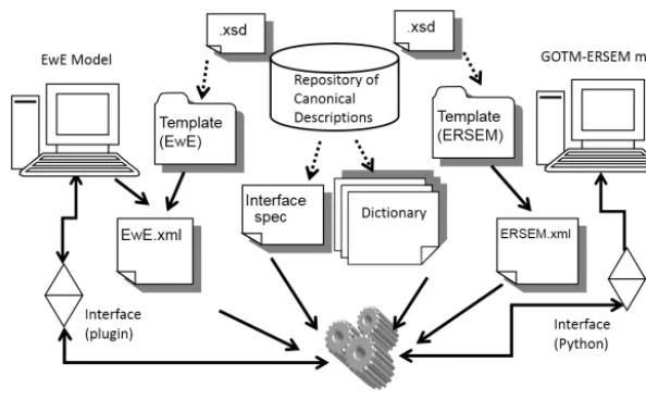
Figure 1. Outline of the information sources in the form of XML files and model components between two models running in network mode with a twin copies of Couplerlib.
a system of extensible mark-up language (XML) files (Fig. 1).
c. Networked coupling (used experimentally in develop-ment): this is an extension of managed coupling, which can operate between processes and across the web. In order to achieve this, there needs to be two copies of Couplerlib with communication processes between each. Typically one of the processes is the master with capabilities for operator interaction and the rest are slaves operating under a system of messages between them. The Atlantis system (http://atlantis.cmar.csiro.au; Fulton, 2010) also implements a networked coupling system between network components but is both data and control central, whereas Couplerlib is control cen-tral and data distributed. Networked coupling would be needed to link an ERSEM model running on a Linux cluster to EwE on a stand-alone PC. Networked cou-pling can be used on the same machine where it is virtu-alized running Linux and Windows or across processes and between processes on the same machine. Couplerlib is typically run from single or synchronous threading, so the results of multiple parallel threads are brought together before conversion to another model. This is seldom a bottleneck where HTL models, specifically Ecosim, are concerned because they typically have a long time step of over a day, compared to a few min-utes in LTL models.
d. Offline coupling (used in subsequent development of three-dimensional models) uses some form of file to store data so that multiple models can run, store data, and allow a second model to process this model inde-pendently. Because of the slow nature of file reading, Couplerlib implements offline coupling using netCDF files as a one-way only coupling. Whilst limited in not
being bidirectional, it is often used for short-term mod-els with limited effects of HTL components on the nu-trient levels.
Couplerlib can be used to link models one way, in which case the values of quantities in the source model overwrite the re-spective quantities in the destination model, or bidirection-ally (not for offline coupling) in which case quantities are passed back from the destination model and re-overwrite the values in the source model. In this way calculation is shared between models and double accounting needs to be avoided, for example, by allowing consumption and not production in the destination model and consumption only in the source model.
2.2 Couplerlib design and specifications
A critical feature of Couplerlib is its ability to specify mul-tiple models and interfaces between them and perform vali-dation on these interfaces, only validated interfaces may link and exchange data. The principle behind this is that multiple coupling mechanisms may be provided, only some of which may be allowed in each situation. An example would be the provision of data in multiple types of grid and non-grid spa-tial formats, which might require a conversion layer between the models; by specifying multiple models we can allow code for multiple conversion libraries to be incorporated within a model.
case it is necessary to develop a coupling mechanism where metadata information that is generated at runtime can still be cross-matched and validated. The mechanism as shown in Fig. 1 is for the user to specify a linkage in terms of models, variables, and quantities (metadata) in XML, which is parsed by the Couplelrib system to build the linkages between mod-els.
For linking to EwE, which is Windows only, managed cou-pling is only possible within a Windows environment. The data store in Couplerlib is global and persistent, and is refer-enced by an enumeration (i.e. a list of items that is converted to a numeric sequence) of model and interface. In princi-ple a single Couprinci-plerlib can be used to link multiprinci-ple models with multiple connections for different types of data between them; however, this was restricted to two (intake and offtake) for this work. However, care must be taken to ensure that a frame of data (data for single model and interface combina-tion) is only read after it is completely written; otherwise, the data may be corrupted. Because programming libraries for multi-threaded systems have various ways to signal events and suspend program execution on a thread, these mecha-nisms need to be provided by the interface to Couplerlib. The strength of Couplerlib is that once this interface code is writ-ten it can be used over and again for different Ecosim models. This threaded mode of interfacing also allows the graphical interface of both models to run simultaneously.
When Couplerlib operates in networked mode, each pro-cess or machine is required to have its own Couplerlib. The networked Couplerlibs are initially synchronized by reading metadata descriptions of all the models being linked from files that will be available on all machines as a Uniform Re-source Identifier (Berners-Lee et al., 2005). At run time the networked Couplerlibs are synchronized on a need-to-know, object request basis (the receiving Couplerlib specifies what data the transmitting Couplerlib needs to send) even though validation has been carried out during the initial model load-ing phase. Data from a model are written to the local copy of Couplerlib and the remote copy synchronizes its own copy when an instruction is received to fetch data. In addition to transferring data, the networked Couplerlib exchanges diag-nostics and model output to be displayed remotely and con-trols the synchronization of data.
To ensure that coupled models are synchronized, Coupler-lib uses the Berkeley sockets mechanism, specifically block-ing sockets. Sockets form the basis of the internet protocol and are used to ensure that networked services are connected from right source to destination (i.e. two ends that have the same socket number) and can be assigned a number by the user or by the operating system. By assigning each a station number, multiple models can connect using networked Cou-plerlibs.
2.3 Metadata information exchange and specification
Couplerlib is a coupling system that uses a metadata descrip-tion of the model linkage, combined with emitted metadata from the component models and a dictionary of functional group and unit definitions to form a linkage between models. It allows linkages to be described in terms of a functional level of abstraction, without the user needing to understand computer representation (such as indexing of arrays) and in many cases without altering code.
Both EwE and GOTM–ERSEM are reconfigurable mod-elling frameworks, which can emit metadata to describe their composition. In the case of GOTM–ERSEM, the output data to be emitted are partly specified by a user specified list of variables, which are then mapped into the main data array (known internally as the CC array) at source level, with pa-rameter values being loaded from a FORTRAN namelist. The physics–LTL model GOTM has an optional front end Graph-ical User Interface (GUI) interface containing a parameter editor, and the model specification can be adjusted during the data editing phase before the core GOTM program starts up. GOTM–ERSEM has an internal array of metadata, which describes the model’s internal arrays in terms of full name, abbreviated name, and unit dimensions, which is created for each instantiation of the source code at the same time as the CC array and describes internal as well as output variables. The Ecopath, Ecosim, and Ecospace programs also have a main data array where metadata is stored, although dimen-sional information is specified for all data items together. This data array can be changed at runtime by means of the editor built into EwE v6, if organisms are added or deleted, for example.
Consequently, the location in terms of numerical index-ation within the data arrays of the two models is not fixed at runtime. Indeed there is no guarantee that the necessary data for a linked model run will even be available once the simulation starts, since the user may remove a needed com-ponent from their model instance. The first stage of model coupling is for each model to provide a specification of the data available for linking, which it provides between model loading/editing and the start of the run. Each model provides this information in XML format. The data are supplied in a hierarchical manner, suitable for reading with the Document Object Model library (Le Hégaret et al., 2009) with the fol-lowing hierarchy:
<Model>
<Description>Author, System, Languages
<Interface>
<Time Information>Periodicity, Start and Stop Times
<DataItems>of type Phytoplankton, Zooplankton, Consumers, Resources
<Name> <Symbol>
<Chemical Consituent>Carbon, Nitrogen, Silicate, Phosphorous
<Flux Direction>Concentration, Intake, Offtake, Mortality, Production
<Units> < /Dataitems> < /Interface> < /Model>
Information on the dimensions of values is included in the metadata specification. If the dimension of a coupled variable differs between coupled models, such as density of a nutri-ent per unit volume, versus density per unit area, Couplerlib checks in its conversion dictionary to find an appropriate di-mensional converter and then applies the relevant conversion ratio to all values transferred between the models (in this case multiplying or dividing by water column depth).
The model specification is produced by combining a tem-plate file, which is an XML file describing the basics of each model (such as language and system), with variable-specific metadata provided dynamically by the model after loading/editing. The specifications for the coupled models are combined by use of a coupler specification, which is also an XML file; this specifies the models to be linked as a num-ber of interfaces. The coupler cross-checks for each interface in turn to see whether the connection is permissible. Permis-sible interfaces occur when the model and system informa-tion are permissible, the spatial and temporal dimensions are in range for the data, and there is a registered correspondence between all functional groups specified in the interface; i.e. the groups have the same name, or there is a correspon-dence between groups in the system dictionary (e.g. group Z4 in ERSEM corresponds to Herbivorous mesozooplankton in our EwE model) or a correspondence between multiple groups (e.g. P1 to P5 in ERSEM sum to phytoplankton in our EwE model). So for each organism in the interface there must be a way of obtaining all nutrient concentrations and the time and area of the data must be consistent. The functional groups that are checked are only those which are specified as actually needing to be linked in the interface specification.
Alongside the XML files used for specifying the rules of the interface, XML Schema Definition (XSD) files can be used to validate the vocabulary and patterns of any human written XML file. For example, the XML file will specify the axes used in the grid, whilst an XSD file will specify that a three dimensional grid will require three axis dimensions each of which will need a start co-ordinate, a length, and a resolution. The XSD file is loaded into a XML editor such
as EditiX (www.editix.com) prior to creating or loading an XML file. It can also be located online via a URL, so may reside in a cross-institutional repository. Its use is optional but will reduce run time errors in Couplerlib.
Couplerlib can be extended to the case where the func-tional group values are structured in some way (e.g. age or size). Additional metadata will define the number and speci-fication of age/size classes. However, further conversion code would need to be supplied when one model outputs as size or age structured and only a single biomass value is needed.
However, it will often be the case that there is a dispar-ity between the metadata produced by the two models to be coupled. The simplest is the use of different names by the two models, other situations arise where there is an inexact match of the functional group definitions between the two models: for example, the version of ERSEM used here has five different phytoplankton groups whereas the EwE North Sea model has a single phytoplankton class. It is acceptable, within EwE, to model the relative offtake of all the phy-toplankton groups as a single value if the predation pres-sure on bulk phytoplankton in EwE can be assumed to ap-ply equally to all phytoplankton groups, but the production and consumption of phytoplankton within GOTM–ERSEM vary between phytoplankton groups. In each time step the predation of phytoplankton is returned as a fixed fraction of input phytoplankton and then this fractional reduction is applied as a proportion to all phytoplankton groups in the ERSEM model. Consumption of phytoplankton directly by higher trophic level groups (e.g. Fish Larvae) is a relatively unimportant energy flow in the EwE models we have stud-ied with only 3.2 g m−2year−1out of 60.8 g m−2year−1
2.4 Use of Graphical User Interfaces – model front ends
Both the EwE models and GOTM (and hence GOTM– ERSEM) have GUIs. In the case of EwE the interface is written in the .net programming environment for Windows, and whilst programmed in Visual Basic, it uses an object structure that is fully accessible using Visual C++and C#. The EwE system is runtime extendable using plug-ins that use the .net interface system to extend the object model of the underlying EwE system. plug-ins are dynamically loaded as dynamic link libraries (DLLs) (executable code program extensions, which must be called from another executable). This plug-in architecture is used to couple EwE, via Coupler-lib, to the GOTM–ERSEM front end. The GOTM interface, however, is written in Python, which is an interpreted lan-guage: the interface consists of a set of scripts and modules that require a Python interpreter to run. Accordingly, an in-terpreter is embedded within the EwE plug-in, together with python.net (http://Pythonnet.sourceforge.net): a .net compat-ible application program interface (API) that provides access to the Python interpreter.
The coupler plug-in has a visual interface to select the di-rectory where the coupler description XML files described previously are contained. This launches the Python inter-preter to run the scripts, which collectively make up the GOTM–ERSEM front end. These scripts enable the GOTM and ERSEM configuration files to be manipulated at run time and also for output data to be visualized. In turn, the Python-based front end communicates with the FORTRAN core of GOTM and ERSEM via a C wrapper layer – F2Py (Peterson, 2007). To enable coupling with external models, this layer has been expanded with interfaces for read–write access to relevant FORTRAN data objects, in particular the arrays that describe the values of biogeochemical state variables. Cou-plerlib is available to parse metadata and carry out the kind of managed data conversion described in the previous section. The net result of these various conversion and API layers is that meaningful data objects in GOTM–ERSEM are avail-able from within EwE and vice versa.
2.5 The LTL and HTL models
The one-dimensional GOTM–ERSEM (Burchard et al., 2006) lower trophic level model was set up to represent a site in the Oyster Grounds (a muddy sand site immediately south of the Dogger Bank at 54◦240N, 4◦30E) with
appro-priate water depth (40 m), tidal velocities (M2amplitudes of
30 cm s−1), and meteorological forcing. This parameteriza-tion simulates the annual dynamics of a summer stratified site that is broadly representative of average behaviour over a large area of the central North Sea. Preliminary validation of this model is reported in van der Molen et al. (2012).
The North Sea EwE ecosystem model (Mackinson and Daskalov, 2007) is a spatially averaged representation of the
biomass of food-web components over the whole North Sea (ICES div IVa-c). It consists of 66 functional groups, which are both pelagic and benthic. However, in order to be con-sistent with ERSEM, this 66 was extended by two new de-tritus groups (separating particulate organic matter (POM) into pelagic and benthic components and adding a new fae-cal POM group), making 68 in total. The lower trophic level groups used by both EwE and GOTM–ERSEM for pelagic and benthic components are listed in Table 1.
2.6 The biology of the coupling
The GOTM–ERSEM representation of the physics and pri-mary production and the EwE representation of the higher trophic levels are coupled via biomass of pelagic plankton groups and nutrients returned to the water column via de-tritus (Table 1). Omnivorous zooplankton (Z4 in ERSEM), microzooplankton, bacteria, and phytoplankton (Z5, Z6, B and P1–P5 in ERSEM) are chosen as the coupling groups. The most significant of these links is with omnivorous zoo-plankton, because in shelf seas it forms the principal pathway that connects the energy from the lower trophic food web with the higher trophic level consumers. The link between omnivorous and carnivorous mesozooplankton is handled in Ecosim rather than ERSEM (with predation by carnivorous Zooplankton turned off in ERSEM). This modification (car-ried out by the authors and Piet Rudaji, author of ERSEM) was to increase the stability of carnivorous zooplankton pop-ulations, otherwise there was a tendency for either carniv-orous zooplankton to go extinct over the winter months or for over consumption of phytoplankton late in the year, de-pending on the coefficients of predation of the two meso-zooplankton groups. Nutrients are returned to ERSEM from Ecosim within the particulate, dissolved, and faecal detritus components, which required adding the faecal component in Ecosim. The one-dimensional version of GOTM–ERSEM captures the biogeochemical processes occurring in the water column, describing the plankton ecosystem from incoming solar radiation, via phytoplankton to zooplankton. The EwE model assumes that the biomass of all functional groups is distributed evenly throughout the model domain.
compo-Table 1. ERSEM and EwE function groups mapped
EwE
group nos. EWE group ERSEM group Notes
51 Carnivorous zooplankton Carnivorous mesozooplankton (Z3) but moved to EwE
Copepods
52 Herbivorous and omnivorous zoo-plankton (copepods)
Omnivorous mesozooplankton (Z4) Copepod nauplii, copepodites, microzooplankton
53 Gelatinous zooplankton
54 Large crabs
55 Nephrops
56 Epifaunal macrobenthos (mobile grazers)
Epibenthic predators (Y1) Cross-reference Group
57 Infaunal macrobenthos Filter feeders (epifauna/infauna) (Y3) Deposit feeders (infauna) (Y2)
58 Shrimp
59 Small mobile epifauna (swarming crustaceans)
60 Small infauna (polychaetes) Deposit feeders (infauna) (Y2) Infaunal predators (Y5)
61 Sessile epifauna Filter feeders (epifauna/infauna) (Y3)
62 Meiofauna Meiofauna (Y4)
63 Benthic microflora (incl. Bacteria, protozoa)
Aerobic benthic bacteria (H1) Anaerobic benthic bacteria (H2)
64 Planktonic microflora (incl. Bacte-ria, protozoa)
Microzooplankton (Z5) Heterotrophic flagellates (Z6) Bacteria (B)
nanoflagellates of up to 20 mi-crometre SED (sedimentation equivalent diameter)
65 Phytoplankton (autotrophs) Diatoms (P1) Flagellates (P2) Picophyto-plankton (P3) Large phytoPicophyto-plankton (P4) Small diatoms (P5)
nents are run separately in each model and thus shadow each other. Detritus is returned to ERSEM, but benthic groups are not fed into EwE nor updated in ERSEM. The EwE compo-nent is affected by the temporal variability of the detritus, but not by the immediate variation of benthic conditions input experienced by the ERSEM model (because these are not ex-plicitly coupled). Consequently, the variability of the species that consume benthic components within EwE is less than those that feed heavily via the pelagic route, which was ob-served as rapid annual oscillations of pelagic components of short lifetime and asymptotic increase in solely benthic com-ponents such as epibenthos. The benthos in the HTL model is therefore dominated by the top-down higher trophic level interactions; improvement of the bottom-up influences is de-pendent on improvements of the LTL benthic model within ERSEM that are actively being researched in the LTL mod-elling community.
ERSEM explicitly describes the concentrations of indi-vidual chemical elements (carbon, nitrogen, phosphorous, and, for some functional groups, silicon). However EwE is a biomass only model (the ratios of carbon, nitrogen, and phos-phorous are not considered. Consequently Couplerlib must estimate the stoichometric ratios of EwE model groups, such as detritus, when transferring biomass-based values from
EwE models back to GOTM–ERSEM, so as to conserve biomass. It achieves this by having two detritus pool excre-tions, which match the C : N : P ratios of ingested nutrients and decay, which starts out assuming a Redfield ratio and then adjusts to remove old biomass in the Redfield ratio and accumulated biomass in its new ratio. It is in accordance with the findings of Frigstad et al. (2011) that P concentration in non-autrotrophs could vary seasonality by around 50 % over Redfield, but was averaged over the course of a year to Red-field or slightly above. ERSEM predicted variations of 100 % or more in P composition in Zooplankton in the most extreme conditions.
EwE Core
EwE GOTMLink Plugin
CouplerLib
GOTM Interface
GOTM GUI (Python)
GOTM - ERSEM
Load
Edit
Run
Visu alize Initialize
New
Create Load model GOTM server
Edit Edit scenario Set_step
New
Simulate Simulator
Setup Biovals access Get biovals
Plugin started Ecopath
run initialized
Get I/F address
Run slab
Run step
Biovals access Get biovals
Put I/F
Get I/F Ecosim
initialized
Sub timestep begin Sub timestep
end Put I/F Get I/F
Set biovals
Biovals set
Simulation ending
Simulation
over Terminate
Finalize
Visualize Get I/F
address
Check I/F
A B
A B
A B
A Calls / puts data in B
A fetches data From B Thread at B waits For thread at A
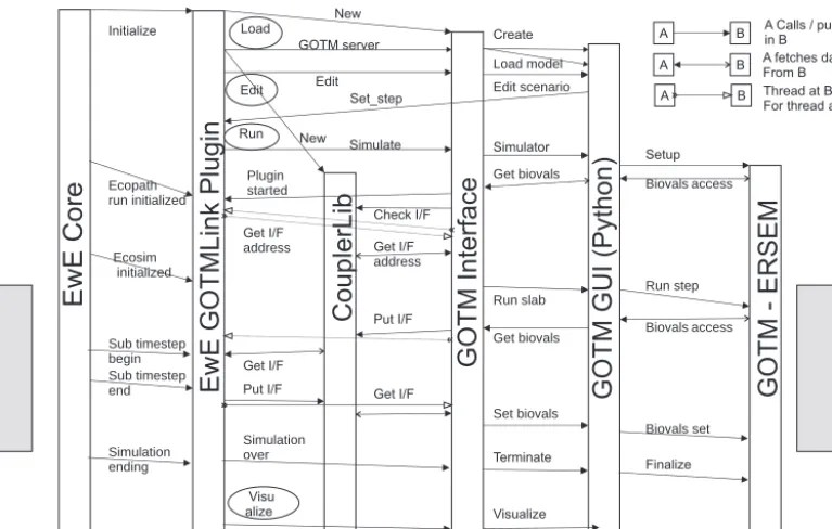
Figure 2. Sequence of operations when GOTM–ERSEM is linked with Ecopath with Ecosim (EwE) in managed model. Grey box is part of model that is run repeatedly on a daily time step.
2.7 The coupling process in action
The main sequence of inter-model calls and data communi-cation is illustrated in Fig. 2. It can be seen that there are six model components. At the ends of the stack of components are the EwE and GOTM models themselves (ERSEM is im-plemented as a library extension to GOTM but is interfaced through GOTM). Furthermore, there is a front end interface to GOTM, which is written in Python and uses the Qt graph-ical interface components (Bruggeman and Bolding, 2007). Although the use of this component is optional, it provides useful online data editing, file management and visualization facilities, so the decision was made to couple the models via the front end to keep the existing functionality.
The six most important points of interface between the core and the GOTMlink plug-in are indicated in Fig. 2, but there are additional points for documentation, identification, and visual interaction with the plug-in. Control passes from the EwE core to the plug-in at those specific points where additional functionality can be provided by the GOTMlink interface. When the two models are coupled in the same pro-cess running on the same machine, the two sides of the model (EwE plus its plug-in and GOTM plus its GUI and Interface) operate on separate threads; that is to say, there are sepa-rate sequences of operations for the EwE and GOTM models. The EwE and GOTM interfaces signal directly when a step in one model is complete and the second model should take over, with execution of the first model suspended in a wait state. Using separate threads is essential where the compo-nent models are themselves multi-threaded and may need to
keep other threads such as the Graphical User Interface or network code running – EwE is like this; GOTM is not like this, but can be embedded within a multi-threaded server, such as a network daemon. Data transfer is carried out by means of Couplerlib, which provides marshalling of the data using external metadata specifications. However, the two in-terfaces can exchange basic information about model status, time to run for, and the like through shared memory.
In networked mode the GOTM and EwE sides cannot communicate directly since they do not share common mem-ory. Instead everything goes via Couplerlib. The EwE and GOTM sides have their own copies of Couplerlib. The two Couplerlibs will exchange information using TCP/IP sock-ets so that the receiving end of a data transfer makes a copy from information requested from the sender Couplerlib. In-formation used to synchronize the models and give informa-tion on the model state, such as waiting, finished, and error conditions for various operation, is sent via a separate pair of sockets and diagnostic information is sent to the Couplerlib, which is attached to the graphical console (the EwE GOTM-link plug-in in this case).
specifi-cation and dictionary to Couplerlib. Data, such as the time step, and the start and stop times are transferred from GOTM to EwE sides (so they can be available before EwE produces its XML metadata). The bulk of the data are transferred via Couplerlib. The critical call to Couplerlib is the CheckIF call, which loads all the metadata specifying the interface, and cross-checks this against the specifications of the component models. Providing this is consistent, the GOTM and EwE threads are synchronized to ensure that the Ecosim module has been started, resulting in the EcoSimRunInitialized call being sent from the EwE core to the plug-in. Both component models can then use GetIFAddress to locate the position of the data that will be transferred in the Couplerlib data store.
The main loop consists of repeated calls to the GOTM li-brary, requesting simulation for a particular length of time, equal to the EwE time step. After every call the GOTM array holding the values of biogeochemical state variables is ac-cessed and its values are stored in Couplerlib. The EwE part of the model will wait for these data to be written, and then fetch the values it requires, using Couplerlib to carry out any conversion between units or between functional groups. Af-ter updating the values of coupled variables in EwE in this fashion, computation continues with the EwE calculations for a single time step. When complete, updated EwE data are written to a different frame of the Couplerlib repository and GOTM must synchronize and then read the data. The changes in biogeochemical state variables during the EwE time step are output to Couplerlib as (dimensionless) relative changes, which can be applied directly across all vertical lay-ers of the GOTM–ERSEM water column without violating mass conservation. Finally, if EwE has finished (the Simula-tion Ending Interface call is made) GOTM can be made to terminate early and cleanup called to ensure data are written to output files.
2.8 EwE model re-parameterization
The very first attempt to link the two models was not success-ful. Pelagic groups that feed off mesozooplankton in EwE overexploited the mesozooplankton during the winter period causing the death of the zooplankton populations and a con-sequent reduction in pelagic productivity. This was a result of the Ecosim model having been calibrated primarily on sum-mer plankton levels to set the consumption to biomass level, albeit annualized i.e. the seasonality in plankton food pro-duction was not captured in EwE (winter zooplankton levels in ERSEM drop to around 1 % of summer ones). In prac-tice consumption is very much lower in winter months when the plankton population is lower but also the basal metabolic rate of the predatory fish is reduced by around a factor of 2.4 compared to summer (Clark and Johnson, 1999). In addi-tion to the reduced metabolism, which follows an exponen-tial temperature to metabolism law, there may be behavioural changes that reduce prey consumption still further. For ex-ample, sandeels, which were observed to be one of the major
predators of mesozooplankton, switch to being benthic be-tween November and April (Engelhard et al., 2008) and so have zero consumption of plankton in winter months. To ac-count for these phenomena, it was necessary to add a func-tion to reduce predafunc-tion of pelagic sources in winter months. Two forcing functions were used – one a purely metabolic model using aQ10=2.0 rule of temperature, with maximum
temperature having a multiplier based on the original EwE model of 1.0, the other fitted the observations on sandeel populations of Engelhard et al. (2008). In addition metabolic costs were reduced to 0.3 for adults and 0.0 for juveniles (this latter figure reflects the seasonal production of juveniles starting in the spring, and their migration from spawning grounds, so there will not be juveniles in the area modelled but the population still needs to be modelled and EwE al-lows only a fixed value for metabolic costs). The background mortality of the zooplankton in ERSEM was reduced to a nominal value to take account of the fact that most mortal-ity would be due to predation, which is accounted for in the EwE model. Interestingly, the level of zooplankton predicted by the ERSEM model peaked at around the value used to calibrate EwE. All of these changes represent a degree of bringing the data to the model and compensating for known limitations of a single model by dampening the damaging effects of assumptions in the underlying model (specifically the low winter zooplankton in ERSEM). In the Discussion we will suggest how this compensation may be addressed in the future.
3 Results
3.1 One-dimensional two-way coupling between LTL and HTL
Here the results from the application of Couplerlib to cou-pling the LTL and HTL models of the North Sea are de-scribed. Results are produced separately but concurrently by the EwE and GOTM–ERSEM parts of the model.
vari-Figure 3. GOTM–ERSEM prediction for the dynamics of four Plankton types – (a) diatoms, (b) flagellates, (c) dinoflagellates, and (d) om-nivorous mesozooplankton within a water column over a 2-year period using synthetic meteorological data 1970–1971.
ation in diatom and dinoflagellate numbers during the sum-mer period.
In Fig. 3d the modelled omnivorous zooplankton dynam-ics are indicated (they are subject to our best guesses as to, in particular, the seasonal mortality of zooplankton, which is a challenge to estimate; Daewel et al., 2014). Between 1970 and 1971 there is a considerable difference in the timing of the peak as a result of differences in the diatom bloom. These differences are likely to have profound, though not completely understood effects on recruitment on pelagic fish in the following year.
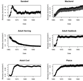
An examination of the effect on a number of functional groups is shown in Fig. 4. Each graph shows the changes in fish population numbers away from the calibrated levels at the start of the simulation (based on the 1990 calibration data); as a result of coupling to the LTL model, the transient effects of the coupling swamp the inter-annual variation to be described later. A significant rebalancing between func-tional groups occurs as a result of the introduction of the sea-sonal lower trophic levels. That the coupled model should give different answers is not surprising, given that (i) there is a switch from a non-seasonal model to a seasonally driven one, (ii) the ERSEM model is calibrated for a single point, the EwE model is for the whole North Sea (iii). It has been shown that for large models small changes in the growth of a single population can have drastic consequences for the pop-ulation of the North Sea (Rossberg, 2013). (iv) Communities are subject to periodic shifts in species within a guild, for example, sardine and anchovy cycles (Chavez et al., 2003). Given these differences between the models we cannot ex-pect a congruency between coupled and uncoupled models,
nor can we predict the likely population of a single species based on meteorological data alone, because it is hard to es-timate recruitment in a mixed-species environment. Never-theless, a stable long-term equilibrium may be found, as the trophic network with Ecosim readjusts. There is a consider-able rebalancing between pelagic groups, for example, her-ring numbers decline (probably a result of the difficulties of modelling this migratory fish in a static model with no space, no larval dynamics, and limited seasonality). We believe that with extensive reworking of the ERSEM and EwE models and extensive recalibration, we can produce a useful operat-ing model to examine how changes in the physical and lower trophic level environment may further affect the ecosystem balance between multiple species.
3.2 Long-term effects of changes in the physical environment on fish biomass
The coupled model was run using synthesized weather data based on the IPCC climate change scenarios A1B (which is a rapid global industrial growth scenario with a mixture of fos-sil and non-fosfos-sil fuels resulting in around 3.2◦of warming)
and B1 (with limited industrial growth and an emphasis on CO2 reduction resulting in 2.4◦ of warming) (Nakicenovic
Figure 4. Dynamics of size commercial fish species under the linked ERSEM–EwE model 1960–2000 simulation.
Table 2. The four parameter settings for the long-term coupled ERSEM EwE model, based on year 2100 IPCC climate change sce-narios.
Scenario N concentration P concentration Warming
A1B1 – High Nut. 10 mmol m−3 1.0 mmol m−3 +3.2◦C A1B1 – Low Nut. 5 mmol m−3 0.5 mmol m−3 +3.2◦C B1 – High Nut. 10 mmol m−3 1.0 mmol m−3 +2.4◦C B1 – Low Nut. 5 mmol m−3 0.5 mmol m−3 +2.4◦C
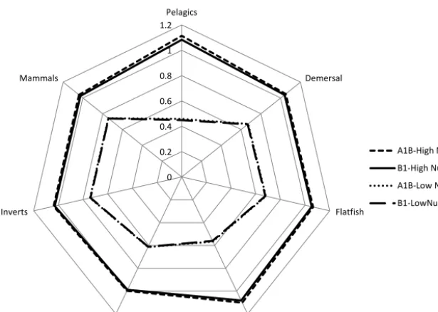
The populations of marine species affected by changes in the environment are grouped in seven blocks: microbes (plankton and bacteria), higher level invertebrates (shrimps, crabs, bivalves, etc.), small and medium pelagic fish (herring, mackerel, sand eels, etc.), demersal fish (cod, haddock, etc., but not flatfish), flatfish (sole, plaice etc. excluding skates and rays), sharks (including skate and rays), and a block con-taining marine mammals and birds. The populations of those species relative to the current temperature and nutrient sce-nario (baseline) in the four scesce-narios for temperature and nu-trients are shown in Fig. 5. It may be seen that the system is very much nutrient limited, especially in pelagic species (where there is a proportional relationship between nutrients and biomass). In large benthic species and mammals the re-lationship is less than linear (i.e. a 30 % reduction in biomass for a 50 % reduction in nutrients). The effect of warming is relatively small and greatest for pelagic species and higher
trophic level predators such as sharks, and negligible for the microbes. The reason for diminution of nutrient effects at higher trophic level effects is that nutrients limit the micro-bial populations whilst increased temperature increases rates of turnover of microbes and hence nutrients, and that there is strong negative feedback on predated populations, which are predated at a higher rate when predator populations increase.
4 Discussion/conclusions
dif-ferent coupling strengths from direct coupling to loose cou-pling via netCDF files. Its main advantage is that the links are made explicit via metadata rather than programming, simple reconciliation of groups and data can be carried out, and it can work across languages and systems including across net-works.
The main disadvantages of Couplerlib (and of the model coupling approach in general) are it is complex to install and that it still requires interface code to integrate into the models to be coupled. The most difficult parts of this project, where getting the threading interaction between the two models GOTM–ERSEM and EwE, which was a specialist program-ming task involving waits and signalling between processes, which occurs in the glue layer between Couplerlib and the model code. This is a task that only has to be done once for each modelling tool, so that the majority of model users would not have to alter code. In a large multi-team project, it is likely that the team will include coders and ecological modelling specialist who can work in their specific domain.
The technical innovation of the coupling processes and the solutions to the ecological problems that emerged has ex-posed both technical and ecological issues of reconciling the two models, the key points of which are discussed below.
In principle Couplerlib is designed to handle coupling of any groups among models, but in this example only the plankton groups are coupled. The reason for this lies in the effort / benefit ratio, the argument being that plankton groups form the main energy conduits through which environmental changes get translated in to changes in secondary produc-tivity, and poor correspondence between the benthic compo-nents of the two North Sea models means a lot of effort would be spent for little marginal gain. Having the dynamics of the benthic components in each model run separately is taken as providing a useful point of comparison.
The example coupling links a one-dimensional LTL model calibrated using parameters from the North Sea Oyster Grounds with the HTL food-web model, whose parame-ters are spatially averaged over the whole North Sea. This discrepancy is related to the more strategic nature of EwE – long-term changes in ecosystem composition versus the more tactical nature of ERSEM – response to environmen-tal transients. While the parameters used to represent each model differ in their degree of spatial specificity, we do not see this giving rise to conceptual or technical issues that can-not be reconciled. First, the Oyster Grounds is a site close to the tidal mixing front that divides summer stratified with the mixed region to the south. Although it simply cannot fully capture the diversity between a mixed site in the south-ern North Sea and a deep strongly stratified location in the northern North Sea, it is nevertheless representative of the dynamics of a large area of the central North Sea. Second, both models utilize many rate and state parameters from a much wider area of the North Sea or are indeed specified even more generally. The internal consistency of each of the separate models might thus imply that each could be
con-sidered as rather general representations of the North Sea ecosystem. From a technical point of view, the practical argu-ments for coupling these non-spatially resolved models are compelling; the coupling allowing proof of concept on the technical methods and early identification of key ecological issues before extending to spatially resolved models. We be-lieve that the main issues have been resolved and plans are in place to tackle coupling spatially resolved models, know-ing full well the new issues will emerge, such as capturknow-ing the dynamics of annual migrations for some species. On the other hand, running ERSEM as a spatial model and aggre-gating over space would help scale up the model.
Plankton growth in ERSEM is regulated by four elements: carbon (C), whose production depends on light and tem-perature, nitrogen (N), phosphorous (P), and silicon (Si). With the particular parameterization chosen for the Oyster Ground model, it has been seen that N is not generally lim-iting, light, as expected, is only limiting during the winter months, and Si and P are more limiting in spring. How-ever, since we have fixed the total amount of these elements and the model is closed, these results are a consequence of our particular choice of initial conditions rather than being a true model prediction. The dynamics of silicon dynamics is more interesting. Particular diatoms, which are more di-gestible by mesozooplankton, bloom in early spring and then are replaced by the flagellates and dinoflagellates as the Si concentration drops, a result consistent with Broekhuizen et al. (1995). The possible biological consequences of this are discussed by Officer and Ryther (1980). One consequence of the Si dependency of diatom production is that Si is only gradually accumulated as a result of inflow from rivers and thus does not change much from one year to the next, so that the total diatom production level is constant from one year to the next although timing of spring bloom will vary from year to year in relation to temperature and light. There is apparent inter-annual variation between the timing of the growth of the different phytoplankton peaks, the importance of which will depend on the ability of zooplankton to incorporate biomass from the different phytoplankton groups. This single point or average model cannot represent the inter-annual variation in phytoplankton bloom location resulting from inter-annual variation in weather combined with ocean currents. For ex-ample, where plankton bloom location varies in space from year to year, the effect on the higher trophic level species will depend on the ability of that species to move with the plankton bloom location.
0 0.2 0.4 0.6 0.8 1
1.2Pelagics
Demersal
Flatfish
Sharks Microbes
Inverts Mammals
A1B-High Nut. B1-High Nut. A1B-Low Nut. B1-LowNut.
Figure 5. Changes in relative biomass of seven classes of functional groups under differing conditions of warming and nutrient availability (see Table 2 for definitions).
the original ERSEM parameterization placed too much em-phasis on the spring diatom bloom as a source of production and so gave a pattern of productivity which did not lead to a stable ecosystem. The current parameterization, which peaks around day 180, gives a better estimate of mean mesozoo-plankton biomass, even though the nutrient model that gives rise to it requires some refinement to fit to observed levels.
There are a number of known divergences from obser-vations for the ERSEM model: for carnivorous zooplank-ton there is under prediction in winter and too great a rise in spring (avoided by moving this group to EwE); and for microzooplankton there is an over estimate of densities (al-though this may be as a result of errors in the observa-tions) (Broekhuizen et al., 1995). Modified EwE parameteri-zations have been made to correct for these: reducing winter metabolism and setting consumption for herring to be very low in winter and adjusting the maintenance cost of herring downwards, in order to prevent this underestimation leading to broader erroneous trophic effects, as a result of erroneous herring deaths. In the long-term improvements to the zoo-plankton component of ERSEM may remove the need for some of these corrections. In the short term these results raise a number of issues about the dynamics of planktivo-rous species such as herring. Given the paucity of zooplank-ton during the winter months, how do they manage to sur-vive over winter? The answers seem to be multifaceted; her-ring switch prey over the winter months (Blaxter and Hunter, 1982), herring are migratory and may move to extend the season of availability of food (Corten, 2000) and herring do seem to exist in a negative energy balance over winter lead-ing to loss of condition. All these aspects are of potentially
great interest for researchers and should be incorporated into future versions of the underlying models.
The time frame of the constituent models is critical to their interoperability. This has often been characterized in terms of time step, but reality is much more complex than that. GOTM is a model that makes use of very high-resolution temporal data, to represent the effects of short-term weather conditions and tides, at a temporal resolution that is sub-hourly. The bio-logical component of ERSEM can respond to these changes in a matter of days because some of the functional groups, for example, bacteria and diatoms can respond over this time frame. In the same way the Ecosim model has these com-ponents with P/B ratios of 30 s year−1or more suggesting that the daily time frame is more appropriate for simulation than the default monthly time frame. However, Ecosim is a model that relies on empirical calibration that is usually an-nual, although some attempts have been made to make sea-sonal Ecosim models with quarterly recalibration (Althauser, 2003). In the current context it would seem that there is a need for seasonal adjustment of parameter values (especially of P/B ratios, basal metabolic rate and starvation mortal-ity). Data for this calibration are not generally available at high frequency, however.
variation in productivity is included (e.g. by coupling models or adding in seasonal forcing), temporal calibration in Eco-path with Ecosim requires consideration of seasonal effects on long-term equilibrium, and given that Ecosim may have multiple equilibria, coupling may cause instability in equi-libria in some circumstances.
Does short-term behaviour matter when considering long-term environmental change? In long-terms of the pelagic system the answer would seem very much to be yes. Over-winter sur-vival of everything from small pelagic fish to seabirds seems to depend upon reserves built up in the previous season, and variation in survival and recruitment is generally considered to be influenced by bottom-up constraints on feeding. In the modelling exercise reported here it was found that overwin-ter survival often depended on sufficiently rapid growth of plankton populations in spring when a fish’s metabolism was increasing. It was necessary to ensure that the forcing func-tions used to limit winter feeding matched the timing of the spring bloom. Further software development could enable this matching to be automatic. This development could be used to model situations, such as the case of Moroccan sar-dine populations, where timing between zooplankton peaks and conditions favourable for spawning influences recruit-ment (Machuo et al., 2009). We can use experirecruit-mental plank-ton studies to make a sensitive calibration of plankplank-tonic re-sponse to short-term meteorological variation, but our ability to explore the effect of climate change on the whole ecosys-tem, particularly its higher trophic level components, and to predict typical weather in future years is very limited.
The addition of a process-oriented model such as GOTM– ERSEM to EwE may allow us to express the relationships between the drivers of change and the consequences. How-ever, the relative insensitivity of EwE to short-term pertur-bations begs a number of questions as to its suitability in studies on the likely consequences of climate perturbations to the ecosystem. First, the fixed seasonality of Ecosim may not adequately represent the results of shifts in the timing of variable onset events such as plankton blooms, but could be incorporated by adding a run time updated forcing function to the feeding via a plug-in within Ecosim. Second, Ecosim is limited in its ability to represent the effect of environmen-tal variation on transient stages of the life cycle of marine organism such as the pelagic larvae of fish and benthic inver-tebrates. This is because of the lack of a model of short-term drivers and components for body condition, and the calibra-tion of the multi-stanza model based on a Von Bertalanfy growth curve, which is based on the growth curve of sharks and does not represent larval stages well (Urban, 2002). The North Sea model calibration, consequently, pays little atten-tion to these stages. Recognising such limitaatten-tions, we are however faced with a practical dilemma; the need for data and modelling tools that help address the pressing research question about how ecosystem respond to change, and the implications for management. The pragmatic route must be
to use the modelling capability we have and use it to help learn how to do better in the future.
Alongside the issue of time is that of space. For some pa-rameter values there were times of the year when either prey or predators became severely depleted because of availabil-ity of prey, but in realavailabil-ity the patchiness of and interconnect-edness of areas with different prey levels would lead to rapid recolonization of the area by new predators and prey. An ex-ample of spatiotemporal local severe depletion was that of the Bay of Biscay anchovy in 2005 (Borja et al., 2008). To address this, an Ecospace model (the spatial equivalent of Ecosim) can be linked to the ERSEM model within GETM, the spatialized version of GOTM; this will allow us to model the temporal shift of marine organisms in response to the spa-tiotemporal dynamics of both marine plankton and fishing pressure. However, spatial biogeochemical models require considerable computational resources to run in most prac-tical situations (typically of the order of a week or more time on a cluster for a 100-year run). The single column GOTM– ERSEM model requires about 90 s year−1 to run on an In-tel i5 processor, and combined with the integrated front end, makes it much more suitable for exploratory parameteriza-tion, teaching, and prototyping than the larger models. The Ecosim model takes under 1 s year−1 to run, it has a time step of 1 day rather than 10 min and has only a single depth layer so that it is calculating less than 1/1000 of the num-ber of time and space elements and Couplerlib is a small proportion of the Ecosim total (less than 10 %), so it is a trivial addition. However, it is less suited to the situation where biological component models such as BFM (biogeo-chemical flux model; http://bfm-community.eu/ last access: 1 March 2016) are being called every short time step across the managed interface. In this case a more direct coupling method such as FABM (framework for aquatic biogeochem-ical models; https://sourceforge.net/projects/fabm/; last ac-cess: 1 March 2016) (Bruggeman and Bolding, 2014) is more suitable, though this will not work across languages and sys-tems in the same way Couplerlib does. Couplerlib can still be used for initial metadata validation, however.
process. The choice of ERSEM for both one-dimensional and three-dimensional modelling is as a result of the use of this model for the North Sea area being examined.
There is considerable debate about whether the compo-nents of end-to-end models should be simple or compli-cated. Very often we are faced with models and sub-models that are both over complicated, in the sense that they con-tain too many parameters and components (Fulton et al., 2003), and over simplistic, in the sense that they contain what can certainly be described as simplifying formulations and may even be seen as dysfunctional formulations (Ander-son and Mitra, 2009). The sterility of this debate has been acknowledged in a number of forums (e.g. the WGIPEM ICES working group http://www.ices.dk/community/groups/ Pages/WGIPEM.aspx) along with the general conclusion dating back to William of Occam that things should be as complicated as necessary but no more so. What are needed, therefore, are not so much simple models as simple conclu-sions that are likely to be robust to uncertain small scale and detailed assumptions and limitations in model formulation. We are a long way off capturing all the physical, biological, and human conditions that will enable us to predict the cod in the North Sea in 50 years, but we at least are starting to have the tools that enable us to integrate important scientific findings within a whole ecosystem context.
In conclusion, linking two very different models has pro-duced a system, which is richly expressive of the kinds of in-teractions of the different functional groups that form pelagic ecosystems and the causes of dynamics, including tempera-ture, nutrient ratios, and biological components of the sys-tem. It is not at this stage very precise (Levins, 1966) because it models a spatial area as a single point in space and because of a number of known limitations not just of the underlying ERSEM and EwE models, but also of spatiotemporal vari-ability of marine data. Nevertheless, the linked model repre-sents a considerable advance on verbal arguments because it can demonstrate the likely relative magnitude of these effects in a wider context of nutrient dynamics and marine fishery management.
Code availability
Source files within this project have been included as fol-lows:
– the source files for the standard C++interface to Cou-plerlib
– the source files for the Managed interface to Couplerlib, which act as a wrapper when called from managed code other than C/C++(especially Visual Basic from EwE) – the source files for the interface between Couplerlib and
EwE
– the XML dictionary, and XML specification files for the GOTM/ ERSEM andEwE models
– parameter namelists for GOTM and ERSEM.
In addition to this, the model will require a complete im-plementation of the GOTM, ERSEM, and EwE models, and third party libraries for netCDF reading, a complete Python interpreter (2.5 to 2.7) with Numpy, Matplotlib, and PyQt4 together with driving data for GOTM (e.g. meteorological data) and the Access database of the relevant EwE model.
This material can be supplied on request but the kind of support needed to commission any non-trivial implementa-tion of an end-to-end model is likely to require considerable time and resources, which can best be provided by third party support.
The Supplement related to this article is available online at doi:10.5194/gmd-9-947-2016-supplement.
Acknowledgements. The authors would like to thank Karsten Bold-ing for advice on the use of the GOTM model, Mark Platts for help in the preparation of the Ecosim figures, and Piet Ruadij for help on understanding the ERSEM components of the model. Many thanks to Villy Christensen, Carl Waters, Sherman Lai, Joe Buszowski, and Jeroen Steenbeek of the EwE team at UBC Vancouver for their aid during my 2 weeks stay in Vancouver and remote support for the plug-in.
This work was funded under the Framework 7, MEECE program (www.meece.eu), Cefas Seedcorn funding, and Defra contract M1202. Useful discussion leading to the development of the model occurred during a workshop of the EasyCo Interreg project (www.project-easy.info).
Edited by: R. Marsh
References
Althauser, L. L.: An Ecopath/Ecosim analysis of an estuarine food web: Seasonal energy flow and response to River-flow related perturbations, MSC Thesis Louisiana State University and Agri-cultural and Mechanical College, 2003.
Anderson, T. R. and Mitra, A.: Dysfunctionality in ecosystem mod-els: an underrated pitfall?, Prog. Oceanogr., 84, 66–68, 2009. Aumont, O., Maier-Reimer, E., Blain, S., and Pondaven, P.:
An ecosystem model of the global ocean including Fe, Si, P co-limitations, Global Biogeochem. Cy., 17, 1060, doi:10.1029/2001GB001745, 2003.
Baretta, J. W., Ebanhoh, W., and Ruardij, P.: The European Regional Seas Ecosystem Model (ERSEM) II, J. Sea Res., 38, 229–483, 1997.