Short‑lag spatial coherence imaging using
minimum variance beamforming on dual
apertures
Yanxing Qi
1, Yuanyuan Wang
1,2*, Jinhua Yu
1,2and Yi Guo
1,2Introduction
Short-lag spatial coherence (SLSC) imaging is a newly proposed beamforming technique for medical ultrasound imaging [1, 2]. Different from traditional beamforming methods, it compounds the spatial coherence rather than the magnitude of the array signal. Com-pared with conventional B-mode methods, the SLSC can better detect lesions inside tis-sues [1]. In addition, it can provide satisfactory contrast and lesion detectability even under a low signal-to-noise (SNR) condition [3]. Previous research has proven that the
Abstract
Background: Short-lag spatial coherence (SLSC) imaging, a newly proposed ultra-sound imaging scheme, can offer a higher lesion detectability than conventional B-mode imaging. It requires a high focusing quality which can be satisfied by the syn-thetic aperture imaging mode. However, traditional nonadaptive synthesis for the SLSC still offers an unsatisfactory resolution. The spatial coherence estimation on the receive aperture cannot fully utilize the coherence information in two-dimensional (2D) echo data.
Methods: To overcome these drawbacks, an improved SLSC scheme with adaptive synthesis on dual apertures is proposed in this paper. The minimum variance (MV) beamformer is applied in synthesizing both the receiving and transmitting apertures, while the SLSC function is estimated on both apertures as well. In this way, the resolu-tion is enhanced by the MV implementaresolu-tion, while the coherence in dual apertures is fully utilized.
Results: Simulations, phantom experiments, and in vivo studies are conducted to evaluate the performance of the proposed method. Results demonstrate that the proposed method achieves the best performance in terms of the contrast ratio (CR), contrast-to-noise ratio (CNR), and the speckle signal-to-noise ratio (SNR). Specifically, compared with the delay-and-sum (DAS) method, the proposed method achieves 42.5% higher CR, 412.7% higher CNR, and 402.9% higher speckle SNR in simulations. The resolution is also better than the DAS and conventional SLSC beamformers. Conclusions: The proposed method is a promising technique for improving the SLSC imaging quality and can provide better visualization for medical diagnosis.
Keywords: Short-lag spatial coherence, Synthetic aperture, Minimum variance, Adaptive beamforming, Ultrasound imaging
Open Access
© The Author(s) 2019. This article is distributed under the terms of the Creative Commons Attribution 4.0 International License (http://creat iveco mmons .org/licen ses/by/4.0/), which permits unrestricted use, distribution, and reproduction in any medium, provided you give appropriate credit to the original author(s) and the source, provide a link to the Creative Commons license, and indicate if changes were made. The Creative Commons Public Domain Dedication waiver (http://creat iveco mmons .org/publi cdoma in/zero/1.0/) applies to the data made available in this article, unless otherwise stated.
RESEARCH
*Correspondence: [email protected]
1 Department of Electronic
SLSC imaging can be applied to clinical research and has the potential of obtaining bet-ter imaging quality [4–6].
The Van Cittert–Zernike theorem is the basis of the SLSC method [2, 7, 8]. It illus-trates that the good performance of the SLSC can only be achieved when the trans-mitted wave is sufficiently focused. In consideration of this principle, a substantial number of conventional imaging modalities are not suitable for the SLSC application. For instance, the commonly used line scan mode can achieve sufficient focus around the focal depth. However, beams are highly diffracted in the near-field and the deep regions, which means that the image quality inside these areas could suffer a severe degradation [9]. This limits the diagnostic value of the SLSC imaging. As another example, the acous-tic wave in the plane wave imaging (PWI) is divergent. Consequently, the combination of the PWI and the SLSC results in poor imaging quality. To meet the requirements of the high focusing quality, it was suggested to apply the synthetic aperture (SA) focusing for the SLSC imaging [9]. Since multitransmission imaging modalities such as the SA imaging and the plane wave compounding (PWC) can naturally achieve the high focus-ing quality by the dynamic aperture focusfocus-ing, the application of the SA imagfocus-ing could improve the SLSC imaging quality mainly in terms of higher contrast [9].
Nevertheless, the inherent drawback of the SLSC imaging still persists. Despite the application of multitransmission modalities, the SLSC images still suffer a lower resolu-tion than convenresolu-tional B-mode ones [3]. To improve the resolution, one way is to modify the physical setup of the SLSC, such as changing the array aperture. Another alternative is to select an appropriate lag value, which is a vital parameter in the SLSC beamform-ing. Previous research confirmed that a large lag value could bring a comparably better resolution [2]. However, a small lag value is commonly adopted for a higher contrast-to-noise ratio (CNR) to distinguish hyperechoic structures. In addition, the small lag value is also necessary for a high SNR [1, 3]. How to make a compromise between the resolu-tion and the CNR is still a conundrum. To pursue a better SLSC imaging quality, several groups including ours proposed some improved algorithms from another perspective [10, 11]. Zhao et al. [11] proposed a novel method which adaptively synthesizes the transmit (Tx) aperture using a minimum variance (MV) beamformer and then calculates the spatial coherence function. According to previous simulations and experiments, the integration of MV and SLSC could bring better resolution and speckle performance, which give us inspiration for further study.
method is conceptually different. Unlike the conventional B-mode MV beamformers with a CF-based postfilter, it is still an SLSC imaging scheme which adopts the MV algorithm for adaptive aperture synthesizing. Second, the spatial coherences are cal-culated in both the Tx and Rx apertures, which fully utilize the coherence informa-tion contained in the 2D data matrix. To evaluate the proposed method, simulainforma-tions, experiments, and in vivo studies are conducted. Results demonstrate that the pro-posed method performs better in the resolution and contrast. Detailed analysis will follow in the sections on results and discussion.
The rest part of this paper is organized as follows: “Backgrounds” section presents
the background of some previous methods. “Methods” section describes the
algo-rithm of the proposed method and the experimental setup. In “Results” section, the simulated and experimental studies are illustrated in detail, including the comparison between different methods. Finally, in “Discussion” section, the improvements of the newly proposed method versus the performance of the conventional B-mode imaging method, as well as the advantages of the former, are discussed, and the conclusions drawn based on the findings of this study with the suggested scope for future study are given in “Conclusion” section.
Backgrounds
Synthetic aperture imaging model
The SA imaging originates from the radar system and is then applied into medical ultrasound imaging [13–15]. In this paper, the synthetic transmit aperture tech-nique is used, which means that only one element fires for each transmitting event. After the propagation through the region of interest (ROI), the backscattered echoes are recorded by all elements. The firing events switch through all transmitting ele-ments to synthesize the full aperture. Suppose an M-element array is adopted, we can acquire an M×M size 2D echo data matrix after all data acquisitions:
where n is the time step and xi,j(n) represents the echo data recorded by the jth element
when using the ith transmitting element. An appropriate time delay is compensated into each channel. In the traditional delay-and-sum (DAS) algorithm, for each imaging point, all channel data are averaged through rows to generate low-resolution images at first. Then these images can be averaged for the final high-resolution image:
where ωR is the receiving apodization window and ωT is the transmitting one. The ni,j
stands for the time index of xi,j(n) , which is calculated by the positions of the
transmit-ting element, the receiving element, and the imaging point.
(1)
X(n)=
x1,1(n) x1,2(n) · · · x1,M(n)
x2,1(n) x2,2(n) . . . x2,M(n)
..
. ... . .. ... xM,1(n) xM,1(n) · · · xM,M(n)
,
(2) zDAS= M1
M
i=1
ωT(i)ziLRI= M12
M
i=1
ωT(i) M
j=1
ωR
Short‑lag spatial coherence algorithm
For echo signals of one single emission, the SLSC imaging algorithm differs a lot from the DAS beamformer. When a transducer array with M elements is adopted, the back-scattered echo arriving at the array after a firing event could be expressed as
where xj(n) represents the echo signal received by the jth element with an appropriated time delay for each channel, n is the time index, and (·)T stands for the matrix transpose. Then the mutual intensity or the so-called spatial coherence between two receiving ele-ments could be estimated from their cross-correlations:
where m is the distance or lag between two elements in terms of number of elements. The temporal sampling kernel n2−n1 is usually shorter than one cycle [2, 3, 9]. The final SLSC value is calculated using the integral of the first q lags:
where q is the number of lags used for summation. An important parameter for the SLSC is Q =q/M × 100%, which is defined as the ratio between the lag number and the element number. Generally speaking, the lower the Q is, the less the high-frequency component is taken into account, which means the contrast would increase, while the resolution could be damaged, and vice versa [2]. Normally the parameter Q is set to range from 10% to 30%, in order to make a compromise between the resolution and con-trast [2, 3].
The SLSC is based on the assumption that the focusing errors due to the acoustic clut-ter mainly influence the correlations of the “short-lag” elements which are closely sep-arated [2]. This assumption illustrates why only signals of closed elements are used to compute the spatial coherence function. Another premise of the SLSC is that the hyper-echoic target and the speckle region have a great difference in their spatial coherence function, which means that a high focusing quality is a prerequisite [2]. The conven-tional line scan ultrasound imaging mode could only ensure the satisfactory focusing quality near the focal zone, while the short-lag coherence function severely decreases in the region far away from the focus [9]. Hence, the SLSC imaging quality suffers a great degradation in these regions. As a solution, the SA imaging modality can help handle this drawback since the SA imaging dataset could be dynamically focused for each imag-ing point. In addition, on the basis of the acoustic reciprocity, the spatial coherence can be calculated in either the synthetic Tx aperture or the Rx aperture [16], which is this paper’s starting point.
Minimum variance beamformer
Adaptive beamformers replace the uniform weight used in the DAS beamformer with a data-dependent weighting vector w(n) for the signal summation. The most (3)
x(n)=[x1(n),x2(n),. . .,xM(n)]T,
(4)
ˆ
R(m)= M−m1 M
−m
i=1
n2
n=n1xi(n)xi+m(n)
n
2
n=n1x2i(n)nn=n2 1x2i+m(n)
,
(5)
RSLSC= q
m=1 ˆ
representative one, MV beamformer, was originally proposed by Capon in 1969 [17]. It calculates the adaptive weights by minimizing the output energy subject to the con-straint that the desired signal is distortionless. Under the incoherent premise between the signal and noise, it is theoretically equal to minimizing the output noise. The MV beamformed output is a product of the received signal vector and the weighting vector:
where x(n) is the echo signal in Eq. (3), w(n) is the MV weighting vector, and (·)H stands for the conjugate transpose. Then the MV beamforming process could be expressed by
where a stands for the steering vector, which can all be assumed as one vector after we
apply the time delay to each channel. R(n) is the covariance matrix of the array data. Using the Lagrange method, the solution to (7) can be calculated as below:
In practice, the covariance matrix R(n) is usually unknown and should be estimated by the temporal array samples. A simple approximation could be R(n)=E
x(n)xH(n)
on the basis of the assumption that the signal and noise are uncorrelated. However, in prac-tical ultrasound imaging, the signal and noise are usually highly correlated. To enhance the robustness, the spatial smoothing is proposed [18, 19]. It divides the array into sev-eral overlapped short subarrays and averages the covariance matrix through all subar-rays. In this way, the on-axis signals can be decorrelated from off-axis ones. The spatial smoothing could be expressed as
where xl=[xl(n),xl+1(n),. . .,xl+L−1(n)]T stands for the lth subarray. L is the
subar-ray length and is usually a little smaller than half of the arsubar-ray size [19, 20]. Another fre-quently used method to improve the robustness is the diagonal loading. It adds a small constant to the original covariance matrix: RDL(n)=R(n)+ε·I , which can make the
covariance matrix nonsingular. Here ε is a small constant, and I is the identity matrix.
The constant ε is often set to be �·trace(R(n)) , while is usually less than 0.1 [19, 20].
Using the modified covariance matrix RDL(n) , the MV weighting vector wMV can be
computed using Eq. (8). Considering the spatial smoothing technique, Eq. (6) should be rewritten to form
Methods
Transmit aperture weighting for the SLSC imaging
The adaptive beamformer can be integrated with the SLSC process. Accordingly, a two-step signal-processing procedure consisting of both the MV process and the SLSC imaging is logically proposed. The SA dataset in “Synthetic aperture imaging model” section, with the
(6)
z(n)=wH(n)x(n),
(7)
min
w w
HR(n)w, subject to wHa=1,
(8)
wMV= R−1a
aHR−1a.
(9)
R(n)= M−1L+1M −L+1
l=1
xl(n)xH
l (n),
(10)
zMV(n)= M−L+11 M−L+1
l=1 wH
appropriate time delay compensation, can be obtained after data collection. The first step is to conduct the adaptive focusing process in the Tx aperture using the MV beamformer. After synthesizing the Tx aperture, the second step is to calculate the spatial coherence in the Rx aperture [11].
In the first step, the 2D echo data matrix is MV beamformed in the Tx dimension to syn-thesize the Rx aperture. To calculate the Tx–MV weights, the covariance matrix of the Tx aperture is averaged through all Rx array elements on the basis of the multiwave beam-forming approach [21, 22]. In addition, since a temporal kernel is adopted in the SLSC algorithm, it is also necessary to adopt the temporal smoothing in the MV process, which averages the covariance matrix through the time index n1 to n2 (the temporal kernel). After
all estimations, the covariance matrix should become as
where xTx
j,l(n)=
xl,j(n),xl+1,j(n),. . .,xl+L−1,j(n)
T
represents the lth Tx subarray of the jth Rx element data. Previous research has proven that the averaging process on both Tx aperture and Rx elements could help increase the accuracy of the estimation, which improves the imaging quality [12, 22]. Then the Tx–MV weight wTx−MV(n) can be calcu-lated by Eq. (8) using the estimated RTx(n) with the appropriate diagonal loading. After the MV weighting process in the Tx aperture, the Tx-synthesized Rx aperture can be written as zRx(n)=
zRx1(n),zRx2(n),. . .,zRxM(n)
, where the Tx-weighted output of a single Rx channel zRxj(n) can be calculated as
The second step is to estimate the spatial coherence through the Rx aperture, namely, the Rx spatial coherence function, RRxˆ (m):
Receive aperture weighting for the SLSC imaging
On the basis of the acoustic reciprocity, the adaptive weighting process can be implemented in both the Tx aperture and the Rx one [16]. In “Transmit aperture weighting for the SLSC imaging” section, the adaptive weighting process is done in the Tx aperture, and the spatial coherence function is calculated through the Rx aperture. Correspondingly, another MV– SLSC process can be implemented. However, this time the Rx aperture focusing process is first conducted using the MV beamformer, and then the SLSC function could be estimated through the Tx aperture. Similarly, the covariance matrix of the Rx aperture is estimated by averaging through not only all Rx subarrays, but also all Tx array elements:
where xRxi,l(n)=
xi,l(n),xi,l+1(n),. . .,xi,l+L−1(n)
T
represents the lth Rx subarray of the ith Tx element data. The Rx–MV weight wRx−MV(n) can also be calculated by Eq. (8). (11)
RTx(n)= 1
(n2−n1)M(M−L+1)
n2
n=n1
M
j=1
M−L+1
l=1
xTxj,l(n)xH Txj,l(n),
(12) zRxj(n)=
1
(n2−n1)(M−L+1)
n2 n=n1 M−L+1 l=1 wH
Tx−MV(n)xTxj,l(n).
(13)
ˆ
RRx(m)= M−1m M−m
i=1
n2
n=n1zRxi(n)zRxi+m(n)
n2 n=n1zRx2i(n)
n2
n=n1zRx2i+m(n)
.
(14)
RRx(n)= (n2−n1)M(M1 −L+1)
n2
n=n1 M
i=1 M−L+1
l=1
xRx i,l(n)x
After the MV weighting process in the Rx aperture, the Rx-synthesized Tx aperture can be written into zTx(n)=
zTx1(n),zTx2(n),. . .,zTxM(n)
, where the Rx-weighted output of a single Tx element zTxi(n) can be calculated as
As mentioned earlier, the spatial coherence can also be estimated through the Tx aper-ture. The Tx spatial coherence function RˆTx(m) can be calculated as follows:
SLSC image formation
The beamforming processes in “Transmit aperture weighting for the SLSC imaging” and “Receive aperture weighting for the SLSC imaging” sections are quite similar, or “sym-metric” in a more precise way. If we transpose the SA data matrix in (1), and then repeat the MV SLSC process described in “Transmit aperture weighting for the SLSC imaging” section on the transposed matrix, we can find that both the procedure and the result are the same as described in the “Receive aperture weighting for the SLSC imaging” sec-tion. It does tally with the acoustic reciprocity mentioned before. There is no precedence in the calculation of the Rx spatial coherence or the Tx one. Both implementations are based on the original echo data (1). Reasonably both Rx and Tx spatial coherence func-tions can be used for the SLSC image formation.
Ordinarily, the SLSC image formation process can be realized through Eq. (5). In this paper, we adopt a modified version to accord with the aperture control technique [11]. The f-number, defined as the ratio between the imaging depth and the effective aperture size, is commonly used to keep a consistent resolution through all depths in medical ultrasound imaging. In this paper’s SA implementation, since the MV weighting pro-cess is conducted in both apertures and so is the SLSC estimation propro-cess, the same f-number value is adopted in both the Tx and Rx apertures in order to make two aper-ture sizes identical. Another reason is to meet the requirements of the reciprocity of the acoustics. An equal size of the transmitting and receiving apertures can maintain the same weight of two apertures in the SLSC calculation, which helps average and reduce the focusing errors in the two apertures. Since the aperture size varies through different imaging depths, the SLSC summation process should be weighted to maintain similar signal magnitudes in the whole imaging region. The modified version of Eq. (5) could be expressed as
Since q is correlated with the imaging depth, the averaging factor 1/q can help keep a consistent signal magnitude in different depths in the final SLSC image.
(15)
zTxi(n)= (n2−n1)(1M−L+1)
n2
n=n1
M−L+1
l=1 wH
Rx−MV(n)xRxi,l(n).
(16)
ˆ
RTx(m)= M1−m M−m
i=1
n2
n=n1zTxi(n)zTxi+m(n)
n2
n=n1z2Txi(n)
n2
n=n1zTx2 i+m(n)
(17)
RSLSC= 1q q
m=1
ˆ
RRx(m)+ ˆRTx(m)
Implementation summary of the algorithm
To make the proposed scheme clear, we give a brief summary of the procedures here.
1. Transform the received radio frequency (RF) data to the in-phase and quadrature (IQ) domains with the appropriate time delay for each channel to obtain the echo data matrix (1).
2. Adaptively synthesize the Tx aperture using the MV beamformer by Eqs. (11) and (12). Then estimate the SLSC function in the Rx aperture using Eq. (13).
3. Accordingly, synthesize the Rx aperture by Eqs. (14) and (15) and estimate the Tx SLSC function using Eq. (16).
4. Sum both the Rx and Tx spatial coherence function by Eq. (17) for the SLSC image formation.
5. Repeat the procedure (1) to (4) for each imaging point.
After all beamforming process, the SLSC image could be directly displayed without a dynamic compression, which is different from the conventional B-mode imaging.
Experimental setup
Both the simulations and experiments were conducted to evaluate the performance of the proposed method. Simulated data were acquired using the Matlab simulation tool Field II [23, 24]. All phantom and in vivo data were generated from the Verasonics ultra-sound platform (V1, Verasonics, Redmond, Washington).
In the Field II simulation, a 5-MHz, 128-element transducer array with a 0.3 mm pitch was adopted. The sampling rate was 40 MHz and a two-cycle sinusoid was used for the excitation pulse. To study the point spread function (PSF), four point targets at z= 30 mm, 35 mm, 40 mm, and 45 mm were first simulated. A 10 dB zero-mean
white Gaussian noise (WGN) was added into each channel to simulate the background noise. In the second simulation, two 2.5-mm radius circular anechoic cysts centered at z= 37 mm and z= 52 mm were simulated. The thickness of the cyst through the y-axis was set to be 8 mm. The speckle region was generated using randomly distributed and random amplitude scatterers with a total amplitude of 10 per wavelength cubic ( 3).
In the phantom and in vivo experiments, a 5-MHz, 128-element linear transducer array with a 0.3 mm pitch (L11-4v, Verasonics, Redmond, Washington, USA) was used. The sampling frequency was originally set to 20 MHz, and the recorded RF data were then resampled at 40 MHz to maintain the same time accuracy with the simulations. All phantom data were obtained using a CIRS calibration phantom (Model 040GSE, Computerized Imaging Reference Systems Inc., Norfolk, Virginia, USA). In vivo human carotid artery data were acquired from a 28-year-old male volunteer.
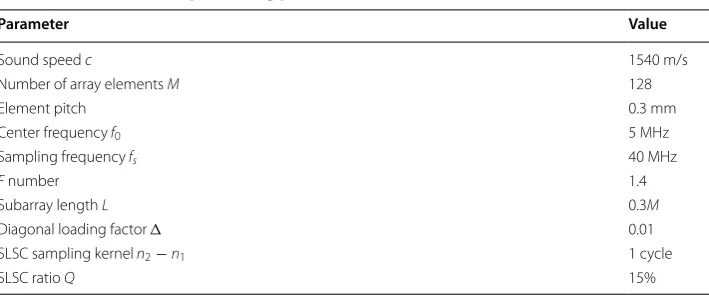
For the SA imaging modality, a spherical wave was transmitted by a single element and recorded by all elements for each emission. The f-number was set to 1.4 using a rectan-gular window for both Tx and Rx apertures. A subarray length of L = 0.3M was used for the spatial smoothing process in the MV algorithm. The diagonal loading parameter
was set to be 0.01. For the SLSC procedure, the ratio Q =q/M was set to be 15% and the
Different results using the DAS, the MV, the SLSC and the proposed DA-MV SLSC are shown together to make an exhaustive comparison. To quantify the performance of different methods, the full-width at half-maximum (FWHM, defined as − 6 dB beam
width for the mainlobe) was adopted for point targets, while the contrast ratio (CR), the CNR, and the speckle SNR were measured for cyst targets. The CR, CNR, and speckle SNR can be calculated by
where µb and µc are the mean signal magnitudes of the speckle and cyst regions, σb and
σc are the standard deviations of the signal magnitude in the speckle and cyst regions,
respectively [2].
Results Simulated study
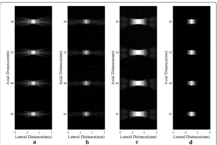
Figure 1 shows images of point targets using different methods. In Fig. 1a, sidelobes are visibly obvious with the DAS beamformer. Using the adaptive MV beamformer, sidelobes could be effectively suppressed in Fig. 1b. The original SLSC result in Fig. 1c seems to be worse than the DAS B-mode image since the points are wider. According to previous research, the wide mainlobe width could occur when the background noise level is very low [3]. As shown in Fig. 1d, the proposed DA-MV SLSC can narrow the mainlobe when compared with conventional SLSC method. The sidelobes are also sup-pressed to a low degree.
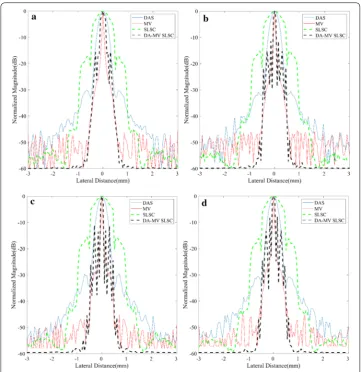
For quantitative measurements, plots of lateral variations of different methods at the depth z= 30, 35, 40 and 45 mm are shown in Fig. 2 while statistical results of corre-sponding FWHMs are presented in Table 2. It is shown that our method achieves better performance than not only the SLSC but also the DAS, which confirms the resolution advantage of the proposed method.
(18)
CR=20 log10(µc/µb),
(19)
CNR= |µb−µc|
σb2+σ2 c ,
(20)
SNR= µb
σb,
Table 1 Transducer and processing parameters
Parameter Value
Sound speed c 1540 m/s
Number of array elements M 128
Element pitch 0.3 mm
Center frequency f0 5 MHz
Sampling frequency fs 40 MHz
F number 1.4
Subarray length L 0.3M
Diagonal loading factor 0.01
SLSC sampling kernel n2−n1 1 cycle
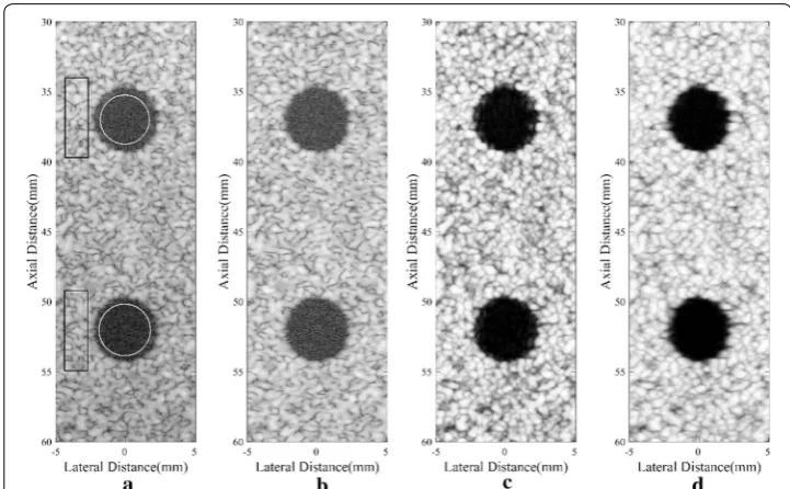
Figure 3 shows images of the simulated anechoic cysts by different beamformers. It could be observed that noises are still at a high level inside the cysts of Fig. 3a, which mainly comes from the sidelobes of the background speckle region. The MV beam-former can slightly suppress the noises while the SLSC can offer an effective noise sup-pression. In the comparison between Fig. 3c, d, both show a good visualization of the anechoic cysts while the boundaries of the cysts in Fig. 3d are more distinct than in Fig. 3c. This indicates the advantage of integrating the MV beamformer with the SLSC algorithm. In Fig. 3d, noises are highly suppressed inside cysts, and the speckle regions are smoother with less dark spots. Generally speaking, the proposed method obtains a satisfactory performance in the cyst simulation.
We measure the CR, CNR, and speckle SNR for both cysts, and the numerical results are shown in Table 3. The corresponding speckle region marked by a black rectangle is selected at the same depth of the cyst marked by a white circle to avoid different attenu-ation through depths [11]. As shown in the results, B-mode MV images do not show much improvement in three metrics. The SLSC method could bring the significant increment mainly in the CNR. In comparison, the DA-MV SLSC can increase three met-rics and get a comparably better performance. Generally speaking, the noise inside cysts is remarkably suppressed by the proposed method, the CR has been notably increased. In addition, the speckle patterns are well preserved, which results in a higher speckle SNR.
Experimental phantoms
Figure 4 shows images of experimental phantoms consisting of two wire targets. The experimental results are similar to the simulated ones in “Experimental phantoms” section. The MV beamformer can obtain a narrower mainlobe width than the DAS
beamformer. The speckle performance of the MV beamformer is also visually better than that of the DAS. For the SLSC beamformer, hyperechoic point targets are visually more detectable, which can be viewed from Fig. 4c, d. In comparison with the original SLSC method, the proposed method obtains better performance mainly in the mainlobe width.
Fig. 2 Lateral variations of different beamformed responses at a z= 30 mm, b z = 35 mm, c z = 40 mm, d
z= 45 mm in the point target simulation
Table 2 Full-width at half-maximum (FWHM) for the beamformed responses
at z= 30/35/40/45 mm
Beamformer FWHM (mm)
DAS 0.42/0.41/0.42/0.41
MV 0.07/0.07/0.07/0.07
SLSC 0.88/0.85/0.90/0.87
Figure 5 plots the lateral variations across the depth z= 19 mm and 28 mm, while sta-tistical results are given in Table 4. The MV gets the narrowest FWHM among all meth-ods. In the SLSC series, the proposed method achieves a good performance just as it does in the point target simulation.
Fig. 3 Simulated anechoic cysts: a DAS, b MV, c SLSC, d DA-MV SLSC. The a and b are B-mode images shown with a dynamic range of 60 dB
Table 3 CR, CNR, and Speckle SNR of the simulated cysts centered at z= 37 mm/52 mm
Beamformer CR (dB) CNR Speckle SNR
DAS − 27.00/− 29.42 1.65/1.91 1.72/1.98 MV − 26.65/− 28.68 1.69/1.90 1.78/1.97 SLSC − 30.03/− 35.39 6.14/7.74 6.40/7.91
DA-MV SLSC − 35.96/− 41.93 8.46/10.31 8.65/10.41
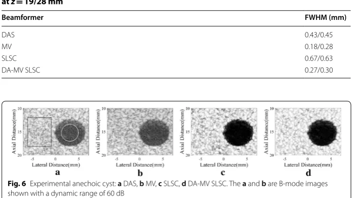
For the anechoic cyst phantom, results are shown in Fig. 6. The improvements of the proposed method mainly happen in less sidelobe noise inside cysts, clearer cyst margins and better speckle performance. Numerical results are presented in Table 5, which are calculated using the anechoic cyst marked by a white circle and its
Fig. 5 Lateral variations of different beamformed responses at a z= 19 mm, b z = 28 mm in the wire target phantom experiment
Table 4 Full-width at half-maximum (FWHM) for the beamformed responses
at z= 19/28 mm
Beamformer FWHM (mm)
DAS 0.43/0.45
MV 0.18/0.28
SLSC 0.67/0.63
DA-MV SLSC 0.27/0.30
Fig. 6 Experimental anechoic cyst: a DAS, b MV, c SLSC, d DA-MV SLSC. The a and b are B-mode images shown with a dynamic range of 60 dB
Table 5 CR, CNR, and speckle SNR of the experimental cyst for different beamformers
Beamformer CR (dB) CNR Speckle SNR
DAS − 28.39 1.81 1.88
MV − 28.23 1.84 1.92
SLSC − 36.71 7.88 8.30
background speckles marked by a black rectangle. Similar to the anechoic cyst sim-ulation, the MV shows no obvious differences in CR, CNR, and speckle SNR when compared with the DAS beamformer. With the SLSC method, the CNR is signifi-cantly increased, and the speckle SNR is also improved, which can be found in results of the SLSC and the DA-MV SLSC. In the comparison between two SLSC methods, the DA-MV SLSC obtains not only higher CR and CNR, but also better speckle SNR. This indicates that the proposed method is effective in suppressing background noises and enhancing the speckle performance.
In vivo study
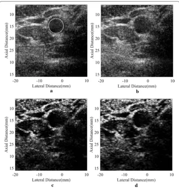
In vivo images of a human carotid artery using different beamformers are presented in Fig. 7. The carotid artery has complicated anatomic structures, but the region inside the blood vessel has similar features with an anechoic cyst. Therefore, the same research pro-cess used in cyst simulations can be adopted to study the performance of these methods. As observed, noises inside the artery are obvious in B-mode images including the DAS
one and the MV one. On the contrary, they are notably removed in the SLSC results. The artery wall can be better defined especially with the DA-MV SLSC. The comparison between the SLSC and the DA-MV SLSC demonstrates that the hyperechoic structures are more distinguishable with our method. The indistinct speckle regions in the original SLSC result are clearer with the proposed DA-MV SLSC, as well, which improves the visualization of the anatomical structures.
Again for the quantitative assessment, the inside-artery regions marked by a white cir-cle and the background speckle marked by a black rectangle are adopted to calculate CRs, CNRs, and speckle SNRs. Corresponding results are given in Table 6. Compared with the original SLSC scheme, the proposed method brings an increased CR, along with a better CNR and speckle SNR.
Discussion
The proposed method is an optimization of the original SLSC method. The utilization of the MV beamforming in both the Tx and Rx aperture is effective in enhancing the imag-ing quality. From the simulated and experimental results, the proposed method obtains a comparably better performance than other beamformers. The resolution and contrast improvements result from two aspects. First, the implementation of the adaptive beam-former (MV) brings a better synthesis for both apertures than the conventional aver-aged compounding, which could further improve the performance of the following SLSC algorithm. The inherent adaptivity of the MV method mainly contributes to the resolution of the output images [20]. In addition, the MV helps remove the off-axis noise around hyperechoic targets, which results in a decline of the spatial coherence in these regions. Since the SLSC process sums all short-lag spatial coherence, the noise part in the final image is also suppressed. Second, the spatial coherence is measured in not only the Rx aperture but also the Tx one, which makes the proposed method different from others. The DA-MV SLSC method is based on the acoustic reciprocity [16]. Thus, there is mutually dual between the beamforming processes in “Transmit aperture weight-ing for the SLSC imagweight-ing” and “Receive aperture weighting for the SLSC imaging” sec-tions. The SLSC estimation in both apertures fully utilizes the coherence information in the synthetic aperture 2D echo data matrix. As a consequence, the contrast is further increased in comparison with the original SLSC scheme. In general, the high contrast along with a better resolution than conventional DAS and SLSC methods indicate that the proposed method could be a promising ultrasound imaging technique for better vis-ualization of the anatomical structures and higher lesion detectability.
As for some parameters used in the proposed method, the subarray length L and the SLSC ratio Q are set to the same value for dual processes in order to accord with
Table 6 CR, CNR, and speckle SNR of the carotid artery for different beamformers
Beamformer CR (dB) CNR Speckle SNR
DAS − 15.20 1.27 1.56
MV − 19.86 1.40 1.56
SLSC − 20.14 1.46 1.70
the acoustic reciprocity. Actually, using different values for the Tx and Rx aperture is also feasible since two processes in “Transmit aperture weighting for the SLSC imag-ing” and “Receive aperture weighting for the SLSC imaging” sections are mutually independent. Changing parameters for one aperture will not affect the beamforming process in another. It is a considerable issue that we can modify the final image by changing both apertures’ parameters separately. It might cause a degradation in the robustness but could bring advantages for specific situations. For instance, when the ROI contains several hyperechoic targets, enlarging L and decreasing Q for the Rx aperture can help achieve a higher contrast and better noise reduction around these targets, while the background speckle region could be damaged.
The computational complexity (CC) of the proposed method is a little higher than those of the MV beamformer and the original SLSC beamformer, since both the MV and the SLSC process are conducted in our method. The MV method has a complex-ity of O
L3
[25, 26], while the CC of the SLSC is comparably similar with that of the MV beamformer [2], also about O
L3
. The proposed scheme includes two MV beam-forming processes and two SLSC estimations, for dual apertures, respectively. Thus, the CC is about four times the original MV methods, but still at the level of O
L3
. In consideration of the application of the graphics processing unit (GPU), it is possible to realize the real-time MV and SLSC algorithm [27–29]. We believe that our method also has the potential for real-time practical implementation.
There are still some unsolved issues in the proposed method. Above all, the inte-gration of the MV and the SLSC could decrease the robustness in complicated situ-ations. The hyperechoic cysts could be indistinguishable from the speckle region using the SLSC scheme. Another problem occurs in the clinical situation. The image enhancement of the proposed method could be influenced by tissue motions, chan-nel noises, and phase aberration. Adopting a compensation technology for the tissue motion could be an effective alternative [30]. Future studies will focus on handling these drawbacks.
Conclusion
We develop a novel SLSC imaging method adopting the MV adaptive synthesis on dual apertures in this paper. The synthetic aperture echo dataset is adaptively beamformed in the Tx and Rx apertures, and the spatial coherence is also estimated through both apertures. Simulated, phantom and in vivo data are collected to demonstrate the advan-tages of the proposed method. Results show that our method can enhance the image resolution which is usually damaged by the original SLSC algorithm. More than this, the CR and speckle SNR are also increased due to the utilization of the adaptive focusing process. Therefore, we consider that the proposed method could be a promising SLSC imaging technique for the better imaging quality in medical ultrasound imaging.
Abbreviations
Authors’ contributions
Study concept and design (YQ); drafting of the manuscript (YQ); critical revision of the manuscript for important intel-lectual content (YQ, YW, JY, YG); obtained funding (YW, JY, YG); administrative, technical, and material support (YW); study supervision (YW). All authors read and approved the final manuscript.
Author details
1 Department of Electronic Engineering, Fudan University, Shanghai, China. 2 Key Laboratory of Medical Imaging
Com-puting and Computer Assisted Intervention (MICCAI) of Shanghai, Shanghai, China.
Acknowledgements
This work was supported by the National Natural Science Foundation of China (61771143 and 81627804).
Competing interests
The authors declare that they have no competing interests.
Availability of data and materials
The simulated data and the experimental data used in this study are available from the corresponding author upon request after the publication of this article.
Consent for publication
Not applicable.
Ethics approval and consent to participate
Informed consent was obtained from the all individual participants included in the study.
Funding
This study was funded by the National Natural Science Foundation of China (61771143 and 81627804).
Publisher’s Note
Springer Nature remains neutral with regard to jurisdictional claims in published maps and institutional affiliations.
Received: 16 March 2019 Accepted: 14 April 2019
References
1. Dahl JJ, Hyun D, Lediju M, Trahey GE. Lesion detectability in diagnostic ultrasound with short-lag spatial coherence imaging. Ultrason Imaging. 2011;33(2):119–33. https ://doi.org/10.1177/01617 34611 03300 203.
2. Lediju MA, Trahey GE, Byram BC, Dahl JJ. Short-Lag spatial coherence of backscattered echoes: imaging characteris-tics. IEEE Trans Ultrason Ferroelectr Freq Control. 2011;58(7):1377–88. https ://doi.org/10.1109/tuffc .2011.1957. 3. Bell MAL, Dahl JJ, Trahey GE. Resolution and brightness characteristics of short-Lag spatial coherence (SLSC) images.
IEEE Trans Ultrason Ferroelectr Freq Control. 2015;62(7):1265–76. https ://doi.org/10.1109/tuffc .2014.00690 9. 4. Bell MAL, Goswami R, Kisslo JA, Dahl JJ, Trahey GE. Short-lag spatial coherence imaging of cardiac ultrasound data:
initial clinical results. Ultrasound Med Biol. 2013;39(10):1861–74. https ://doi.org/10.1016/j.ultra smedb io.2013.03.029. 5. Jakovljevic M, Trahey GE, Nelson RC, Dahl JJ. In vivo application of short-lag spatial coherence imaging in human
liver. Ultrasound Med Biol. 2013;39(3):534–42. https ://doi.org/10.1016/j.ultra smedb io.2012.09.022.
6. Kakkad V, Dahl JJ, Ellestad S, Trahey G. In vivo application of short-lag spatial coherence and harmonic spatial coher-ence imaging in fetal ultrasound. Ultrason Imaging. 2014;37(2):101–16. https ://doi.org/10.1177/01617 34614 54728 1. 7. Mallart R, Fink M. The Van Cittert-Zernike theorem in pulse echo measurements. J Acoust Soc Am. 1991;90(5):2718–
27. https ://doi.org/10.1121/1.40186 7.
8. Walker WF, Trahey GE. Speckle coherence and implications for adaptive imaging. J Acoust Soc Am. 1997;101(4):1847–58. https ://doi.org/10.1121/1.41823 5.
9. Bottenus N, Byram BC, Dahl JJ, Trahey GE. Synthetic aperture focusing for short-lag spatial coherence imaging. IEEE Trans Ultrason Ferroelectr Freq Control. 2013;60(9):1816–26. https ://doi.org/10.1109/tuffc .2013.2768.
10. Chau G, Lavarello R, Dahl JJ. Short-lag spatial coherence weighted minimum variance beamformer for plane-wave images. In: IEEE International Ultrasonics Symposium, Tours, France, 18–21 September 2016:1–3. https ://doi. org/10.1109/ultsy m.2016.77288 89.
11. Zhao J, Wang Y, Yu J, Guo W, Zhang S, Aliabadi S. Short-lag spatial coherence ultrasound imaging with adaptive syn-thetic transmit aperture focusing. Ultrason Imaging. 2017;39(4):224–39. https ://doi.org/10.1177/01617 34616 68832 8. 12. Zhao J, Wang Y, Zeng X, Yu J, Yiu BYS, Yu ACH. Plane wave compounding based on a joint transmitting-receiving
adaptive beamformer. IEEE Trans Ultrason Ferroelectr Freq Control. 2015;62(8):1440–52. https ://doi.org/10.1109/tuffc .2014.00693 4.
13. Jensen JA, Nikolov SI, Gammelmark KL, Pedersen MH. Synthetic aperture ultrasound imaging. Ultrasonics. 2006;44:E5–15. https ://doi.org/10.1016/j.ultra s.2006.07.017.
14. Hemmsen MC, Rasmussen JH, Jensen JA. Tissue harmonic synthetic aperture ultrasound imaging. J Acoust Soc Am. 2014;136(4):2050–6. https ://doi.org/10.1121/1.48939 02.
15. Kortbek J, Jensen JA, Gammelmark KL. Sequential beamforming for synthetic aperture imaging. Ultrasonics. 2013;53(1):1–16. https ://doi.org/10.1016/j.ultra s.2012.06.006.
• fast, convenient online submission
•
thorough peer review by experienced researchers in your field
• rapid publication on acceptance
• support for research data, including large and complex data types
•
gold Open Access which fosters wider collaboration and increased citations maximum visibility for your research: over 100M website views per year
•
At BMC, research is always in progress.
Learn more biomedcentral.com/submissions
Ready to submit your research? Choose BMC and benefit from: 17. Capon J. High-resolution frequency-wavenumber spectrum analysis. Proc IEEE. 1969;57(8):1408–18. https ://doi.
org/10.1109/proc.1969.7278.
18. Shan TJ, Wax M, Kailath T. On spatial smoothing for direction-of-arrival estimation of coherent signals. IEEE Trans Acoust Speech Signal Process. 1985;33(4):806–11. https ://doi.org/10.1109/tassp .1985.11646 49.
19. Synnevag J-F, Austeng A, Holm S. Adaptive beamforming applied to medical ultrasound imaging. IEEE Trans Ultra-son Ferroelectr Freq Control. 2007;54(8):1606–13. https ://doi.org/10.1109/tuffc .2007.431.
20. Synnevag J-F, Austeng A, Holm S. Benefits of minimum-variance beamforming in medical ultrasound imaging. IEEE Trans Ultrason Ferroelectr Freq Control. 2009;56(9):1868–79. https ://doi.org/10.1109/tuffc .2009.1263.
21. Jensen AC, Austeng A. An approach to multibeam covariance matrices for adaptive beamforming in ultrasonogra-phy. IEEE Trans Ultrason Ferroelectr Freq Control. 2012;59(6):1139–48. https ://doi.org/10.1109/tuffc .2012.2304. 22. Rabinovich A, Friedman Z, Feuer A. Multi-line acquisition with minimum variance beamforming in medical
ultra-sound imaging. IEEE Trans Ultrason Ferroelectr Freq Control. 2013;60(12):2521–31. https ://doi.org/10.1109/tuffc .2013.2851.
23. Jensen JA, Svendsen NB. Calculation of pressure fields from arbitrarily shaped, apodized, and excited ultrasound transducers. IEEE Trans Ultrason Ferroelectr Freq Control. 1992;39(2):262–7. https ://doi.org/10.1109/58.13912 3. 24. Jensen JA. Field: a program for simulating ultrasound systems. Med Biol Eng Comput. 1996;34(Suppl. 1, Pt. 1):351–3. 25. Zeng X, Chen C, Wang Y. Eigenspace-based minimum variance beamformer combined with Wiener postfilter for
medical ultrasound imaging. Ultrasonics. 2012;52(8):996–1004. https ://doi.org/10.1016/j.ultra s.2012.07.012. 26. Golub GH, Van Loan CF. Matrix computations. Baltimore: Johns Hopkins University Press; 2012.
27. Asen JP, Buskenes JI, Colombo Nilsen IC, Austeng A, Holm S. Implementing Capon beamforming on a GPU for real-time cardiac ultrasound imaging. IEEE Trans Ultrason Ferroelectr Freq Control. 2014;61(1):76–85. https ://doi. org/10.1109/tuffc .2014.66897 77.
28. Yiu BYS, Yu ACH. GPU-based minimum variance beamformer for synthetic aperture imaging of the eye. Ultrasound Med Biol. 2015;41(3):871–83. https ://doi.org/10.1016/j.ultra smedb io.2014.11.005.
29. Hyun D, Trahey GE, Dahl JJ. In vivo demonstration of a real-time simultaneous B-mode/spatial coherence GPU-based beamformer. In: IEEE international ultrasonics symposium, Prague, Czech Republic, 21–25 July 2013:1280–3. https ://doi.org/10.1109/ultsy m.2013.0327.