https://doi.org/10.5194/gmd-10-2525-2017 © Author(s) 2017. This work is distributed under the Creative Commons Attribution 3.0 License.
A radiative transfer module for calculating photolysis rates and
solar heating in climate models: Solar-J v7.5
Juno Hsu1, Michael J. Prather1, Philip Cameron-Smith2, Alex Veidenbaum3, and Alex Nicolau3 1Department of Earth System Science, University of California Irvine, Irvine, California, 92697, USA 2Lawrence Livermore National Laboratory, Livermore, California, 94551, USA
3Department of Computer Science, University of California Irvine, Irvine, California, 92697, USA
Correspondence to:Juno Hsu ([email protected])
Received: 31 January 2017 – Discussion started: 8 February 2017
Revised: 25 May 2017 – Accepted: 30 May 2017 – Published: 3 July 2017
Abstract. Solar-J is a comprehensive radiative transfer model for the solar spectrum that addresses the needs of both solar heating and photochemistry in Earth system mod-els. Solar-J is a spectral extension of Cloud-J, a standard in many chemical models that calculates photolysis rates in the 0.18–0.8 µm region. The Cloud-J core consists of an eight-stream scattering, plane-parallel radiative transfer solver with corrections for sphericity. Cloud-J uses cloud quadrature to accurately average over correlated cloud layers. It uses the scattering phase function of aerosols and clouds expanded to eighth order and thus avoids isotropic-equivalent approx-imations prevalent in most solar heating codes. The spectral extension from 0.8 to 12 µm enables calculation of both scat-tered and absorbed sunlight and thus aerosol direct radiative effects and heating rates throughout the Earth’s atmosphere.
The Solar-J extension adopts the correlated-k gas ab-sorption bins, primarily water vapor, from the shortwave Rapid Radiative Transfer Model for general circulation model (GCM) applications (RRTMG-SW). Solar-J success-fully matches RRTMG-SW’s tropospheric heating profile in a clear-sky, aerosol-free, tropical atmosphere. We compare both codes in cloudy atmospheres with a liquid-water stratus cloud and an ice-crystal cirrus cloud. For the stratus cloud, both models use the same physical properties, and we find a systematic low bias of about 3 % in planetary albedo across all solar zenith angles caused by RRTMG-SW’s two-stream scattering. Discrepancies with the cirrus cloud using any of RRTMG-SW’s three different parameterizations are as large as about 20–40 % depending on the solar zenith angles and occur throughout the atmosphere.
Effectively, Solar-J has combined the best components of RRTMG-SW and Cloud-J to build a high-fidelity module for the scattering and absorption of sunlight in the Earth’s at-mosphere, for which the three major components – wave-length integration, scattering, and averaging over cloud fields – all have comparably small errors. More accurate solutions with Solar-J come with increased computational costs, about 5 times that of RRTMG-SW for a single atmosphere. There are options for reduced costs or computational acceleration that would bring costs down while maintaining improved fi-delity and balanced errors.
1 Introduction
of aerosols and clouds (Boucher et al., 2013). In comparison, relatively little attention has been paid to improving the treat-ment of aerosol and cloud scattering in climate models. This is both surprising and not. Solutions of the radiative trans-fer (RT) equations in scattering media are well documented with numerous methods and readily available packages such as TUV (Tie et al., 2003; Palancar et al., 2011) and SCIA-TRAN (Rozanov et al., 2014). However, these more accurate reference codes have always been viewed as too computa-tionally expensive. In terms of climate model development, this is a solved problem with little intellectual interest but is too onerous to improve, and thus low-order approximations remain in place.
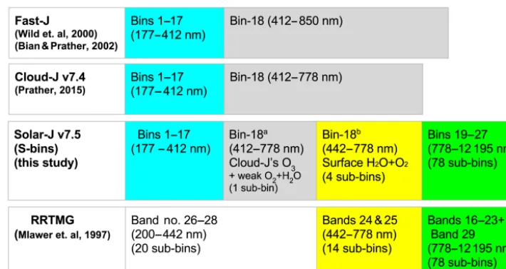
We present here Solar-J version 7.5, a radiative trans-fer model based on the computationally optimized photol-ysis code, Cloud-J (Prather, 2015). Cloud-J combined an im-proved cloud overlap algorithm based on observed decorre-lation lengths with the cloud quadrature scheme (Neu et al., 2007) for averaging over independent column atmospheres. It includes an eight-stream scattering photolysis code with semi-spherical geometry and wavelength integration over 18 spectral bins from 177 to 850 nm. In the most recent version (v7.4), the spectrum was shortened to 778 nm (see Fig. 1). Prior released versions, known in the community as Fast-JX or simply Fast-J (see Søvde et al., 2012; Telford et al., 2013; Sukhodolov et al., 2016), were based on the work of Fast-J2 (Bian and Prather, 2002) and the original Fast-J (Wild et al., 2000), separately optimizing the absorptions of photon fluxes into 12 stratospheric bins (177–292 nm) and seven tropospheric bins (292–850 nm). Although this is the first version of Solar-J, we retain the numbering of the re-leased versions of the core photolysis code. For simplicity, we will refer to Cloud-J, not Fast-J, as the starting point of Solar-J throughout the text. The accurate treatment of cloud and aerosol scattering has been an essential requirement for atmospheric chemistry modeling, and Cloud-J or alterna-tive models (fast-TUV, Tie et al., 2003) are used standardly in global chemistry models. Solar-J is an extension of the Cloud-J wavelength range (0.18–0.8 µm) out to 12 µm and in-cludes an eight-stream scattering solution for the absorption and reflection of sunlight over the full spectrum. Scattering and absorption by large aerosols (dust) and clouds are impor-tant for heating rates at these longer wavelengths. The long-term goal is to develop Solar-J as a single module for climate models, albeit with increased computational cost, delivering photolysis rates and more accurate shortwave heating rates, particularly for aerosol and cloud radiative forcing.
As finer grid resolutions and massively parallel comput-ing are becomput-ing pursued to enable more realistic atmospheric interactions with the land, ocean, and biosphere in climate modeling, the radiative transfer codes implemented in most of the global models remain in their simplest possible analyt-ical form of two-stream scattering. With this approximation, all upward and downward scattering occurs at a single angle, and the scattering must be treated as isotropic, i.e.,
indepen-dent of sun angle. The ubiquitous adoption of two-stream RT codes by the global climate and weather-forecasting mod-els (e.g., the US Department of Energy (DOE) Accelerated Climate Modeling for Energy (ACME), the National Cen-ter for Atmospheric Research (NCAR) Community Earth System Model (CESM), the European Centre for Medium-Range Weather Forecasts (ECMWF) model) has been en-abled by standardized packages like the Rapid Radiative Transfer Model for general circulation model (GCM) appli-cations (RRTMG), developed based on the correlated-k ap-proach (Mlawer et al., 1997; Clough et al., 2005). A two-stream model was certainly necessary at a time when the need for computational efficiency exceeded that for accuracy. With the rapid advancement of massively parallel comput-ing, it is time to ask if an upgrade to a higher-order scheme is needed for improved accuracy in climate modeling, par-ticularly with regard to cloud and aerosol forcing. The two-stream scattering approximation has been in use for decades in climate models and evaluating its systematic errors re-mains an active research topic (Li et al., 2015; Barker et al., 2015). The errors are mostly from the inadequacy of using a single angle to represent the scattering of cloud particles and aerosols. For example, the anisotropic, forward-peaked scattering of all relevant atmospheric aerosols and cloud par-ticles cannot be represented with the two-stream approach, and all scattering must be reduced to isotropic. To address this problem, a commonly used delta-scaling technique is applied by removing the large forward-scattering peak, thus reducing the optical depth (Joseph et al., 1976; Wiscombe, 1977). In addition, the Henyey–Greenstein (HG) phase func-tion (Henyey and Greenstein, 1941) is often used to tune the two-stream scattering to better represent the scattering of large particles for specific sun angles. Unfortunately, the HG phase function lacks the realistic back-scattering peak found for cloud particles, particularly ice crystals (Zhou and Yang, 2015). Li et al. (2015) find biases caused by the HG phase function and conclude that higher-order moments of the phase function coupled with a multi-stream radiative trans-fer algorithms are needed to improve accuracy. They demon-strate this point with a four-stream delta-Eddington code de-veloped by Li and Ramaswamy (1996). Wild et al. (2000) tested the accuracy of different-order codes for computing the mean radiation field in the presence of thick water clouds and found that eight streams were necessary to have errors of only a few percent relative to a 160-stream code that re-solved the scattering phase function. For Solar-J, we adopt the Wild et al. (2000) optimization for water clouds and use Mie (liquid) or Mishchenko (ice) (Mishchenko et al., 1996, 2004) full phase functions for scattering, truncate the expan-sion in Legendre polynomials to order 8, and solve the scat-tering with eight streams with no delta scaling of the optical depth.
Figure 1.Solar-J extends Cloud-J’s solar wavelength bands by combining and modifying RRTMG-SW’s bands 24 and 25 (442–778 nm) and adopts all RRTMG’s bands longwards of 778 nm (see text for details).
RRTMG-SW. Section 4 examines computational costs for Solar-J and options for optimization. Conclusions and a path forward are discussed in Sect. 5.
2 Methods: model configuration and test cases
2.1 Solar-J spectral configuration
The 18 bins of Cloud-J make up the first 18 bins of Solar-J and were optimized for calculating photolysis rates below 64 km (Wild et al., 2000; Bian and Prather, 2002). The first 11 bins (177–291 nm) are optimized around the Schumann– Runge bands of O2 and the Hartley bands of O3, and the next 7 bins are optimized for tropospheric photolysis (291– 778 nm). The bins were chosen to have relatively uniform opacities for the principal absorbing species O2 and O3 across the wavelengths in each bin. In some cases, this in-cludes combining different wavelength regions on either side of the O3maximum cross section near 255 nm. Effectively, the 18 bins extend the use of opacity distribution functions used to calculate O2photolysis rates in the Schumann–Runge bands (Fang et al., 1974), an equivalent to the correlated-k method in the infrared (Lacis and Oinas, 1991). An inherent assumption is that any other scatterers and absorbers are uni-form across each wavelength bin, justified by the narrowness of the bins and the lack of sharp spectral features in clouds and aerosols. Because Cloud-J has been optimized against high-resolution spectral data for stratospheric ozone photol-ysis and continually updated with new cross sections (Sander et al., 2011), and tested against other codes (Palancar et al., 2011; PhotoComp, Eyring et al., 2010), we have confidence in our stratospheric photolysis and heating rates.
The large bin 18 (412–778 nm) that includes the O3 Chap-puis band is unusual for Cloud-J: it assumes a uniform ab-sorption cross section for O3, and it has a large, factor of 2 change in wavelength. The O3cross sections vary smoothly over bin 18 and are>0.5×10⁻²¹cm2over the range 475– 725 nm with a broad maximum of 5×10⁻²¹cm2 about 600 nm. Overhead opacity ranges from 0.4 to 4 % over this band. With optically thin absorption, one can use the flux-weighted average cross section, 1.94×10⁻²¹cm2, for the en-tire bin. Both the attenuation of sunlight and the absorption of photons to calculate the O3photolysis rate use this aver-age. At very large air masses (solar zenith angles of 89–95◦) the atmospheric path (vertical optical path×1/cos(SZA)) in the Chappuis band approaches 1 and modest errors appear. If highly accurate calculation of the photolysis and heat-ing rates due in the Chappuis band is required, then fur-ther analysis of bin 18 is warranted, but ofur-therwise this treat-ment is sufficiently accurate to follow these rates as the sun sets. Another possible source of error is that these cross sec-tions are photon weighted, and for heating rates the cross sections should be energy weighted (W m−2). Fortunately, the energy-weighted O3cross section, 1.91×10⁻²¹cm2, dif-fers little from the photon-weighted one (with the result of <0.04 K day−1 difference in clear-sky stratospheric heat-ing).
the transition to RRTMG bins. The flux-weighted cross sec-tions for several Cloud-J species have been recalculated to account for this. Be aware that these rescaled cross sections apply to Cloud-J versions 7.4 and later. Cloud-J remains a key component of Solar-J, as it produces representative sam-ples of independent column atmospheres after considering the topology of cloud fractions (Prather, 2015). Solar-J has 27 major bins, referred to here as S-bins, e.g., S1–S27 in Table 4. Bins S1–S17 are taken directly from Cloud-J and have no sub-bins. The transition bin S18 combines Cloud-J’s uniform treatment of Chappuis-band O3absorption with four small non-overlapping sub-bins (17.5 out of a total of 608.7 W m−2)to include RRTMG’s H2O and O2absorptions from their bins B24–B25. These four sub-bins have strong cross sections with their own distinct optical depth struc-tures, and they do not overlap with the major O3 absorp-tion in bin S18. The rest of the non-ozone sub-bins (weak cross sections) are lumped into one more sub-bin and added to Solar-J’s Chappuis band. In all, we took RRTMG’s 14 sub-bins from B24 and B25 and optimized these into 5 sub-sub-bins for S18. The last 9 bins, S19–S27, are directly implemented from RRTMG and contain 78 sub-bins. The logic of having wavelength bins and then sub-bins within them is to allow the gaseous absorbers with similar opacities to be gathered into one sub-bin but to treat the scattering and absorption by aerosols and clouds as uniform across the major bin (see Sect. 2.2). The fidelity of the spectral extension of Solar-J to match RRTMG-SW is verified with the clear-sky case pre-sented in Sect. 3.1.
2.2 Clouds and aerosols
Like the photolysis rates calculated in Cloud-J, the heat-ing rates in RRTMG-SW and Solar-J are highly sensitive to the scattering and absorption from tropospheric and strato-spheric aerosols, and from liquid-water and ice-water clouds. Cloud-J v7.4 has pre-computed tables of optical proper-ties for typical aerosols and for both liquid- and ice-water clouds. For bins S1–S18, many of these are effectively non-absorbing. With the extension to longer wavelengths, it be-comes important to treat the absorption by clouds and the stratospheric sulfate layer. We take the refractive indices for liquid water, ice water, and sulfuric acid and calculate solar-flux-weighted mean values for each bin (S12–S27). Sunlight over wavelengths for bins S1–S11 does not reach the tropo-sphere in significant amounts, and hence the optical prop-erties of bin S12 are used for S1–S11 for simplicity. For the first 18 bins, optical properties are weighted by the solar pho-ton flux (phopho-tons cm−2s−1), and for the last 9 bins they are weighted by the solar energy flux (W m−2). These refractive indices are combined with a Mie scattering code and a model for the size distribution of particles to calculate the effective radius (re), single scattering albedo (SSA), ratio of optical to geometric cross section (Q), and the first eight terms in the
expansion of the scattering phase function (A0:7)that include the asymmetry parameter (g=A1/3).
For liquid water, we take the refractive index from FOR-TRAN codes developed at the University of Wisconsin– Madison by M. A. Walters for liquid water (NDXWATER: Hale and Querry, 1973; Palmer and Williams, 1974; Down-ing and Williams, 1975) and ice water (NDXICE, based on Warren, 1984). Liquid-water clouds use Deirmendjian’s C.1 gamma distribution of drop sizes (α=6; see Deirmendjian, 1969) and the Mie code from Hansen and Travis (1974) for a range of effective radii:re=1.5, 3, 6, 12, 24, 48 µm; see also Hess et al. (1998). Optical properties (SSA,Q,A0:7,g)
are calculated for bins S12–S27 for these effective radii and then individual cloud properties at each bin are interpolated piecewise linearly inre.
For ice-water clouds, we have two T-matrix computations supplied by M. Mishchenko for Cloud-J (Mishchenko et al., 2004) for warm (irregular) and cold (hexagonal) ice clouds. These includedQand the scattering phase function (includ-ingA0:7)for the visible region (∼600 nm) and were used at all Solar-J wavelengths. When there is significant absorp-tion, the values of SSA, and to some extentQ, are complex functions ofreand do not simply scale as total mass. For this first version of Solar-J, we made a simplifying assumption and used the Mie code with the ice-water refractive index to calculate SSA andQas a function ofre=3, 6, 12, 24, 48, 96 µm using the liquid-water clouds’ C.1 distribution. Effec-tively, we assumed that the ice particles were spheres. For the phase functionA0:7, we kept the two T-matrix results
(irreg-ular and hexagonal ice particles) and used them for allreof that type of ice cloud. The obvious next upgrade to Solar-J is a redo of the ice-water clouds with a broader, better mix of cloud types (Mishchenko et al., 2016; Yang et al., 2015).
and dust is to be accurately modeled with Solar-J, then one must go to the specific models to acquire the physical and optical properties, e.g., NCAR’s CESM 1.2 (Tilmes et al., 2015).
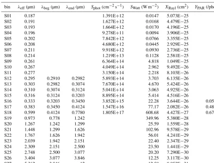
The Solar-J bins, solar fluxes (Sphot in photons cm−2s−1 and SWatt in W m−2), and Rayleigh cross sections (XRaylcm2)are summarized in Table 1. The spectral prop-erties for examples of liquid-water clouds (re=12 µm), ice-water clouds (re=48 µm, cold, hexagonal), background stratospheric 70 wt % sulfuric acid aerosols, and volcanically enhanced stratospheric aerosols for each Solar-J bin are given in Table 2. This table gives wavelength data for the real and imaginary refractive indices based on the flux-weighted means, as well as the Mie-derived values forQ, SSA, andg. The relative importance of cloud heating in each bin can be estimated by multiplying the solar energy by the absorbing fraction,SWatt×(1−SSA). One finds that absorption for bins S1–S20 is negligible, that both types of clouds and strato-spheric sulfate aerosols have large absorption in bins S25– S27, and that ice-water clouds have large absorption per op-tical depth in bins S21–S24 while liquid-water clouds do not. Ice-water and liquid-water clouds have real refractive indices that differ by at most 5 %, and imaginary refractive indices that differ typically by a factor of 2 (except for S27). The cause of this difference in specific absorption is the ratio of mass (which controls absorption) to surface area (which con-trols optical depth), i.e., it is proportional tore, and ice-water clouds typically have 4 times greaterre.
2.3 Test cases: clear-sky, clouds, and the optical properties
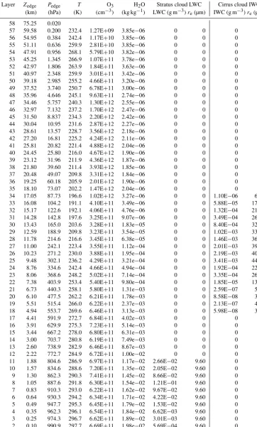
To compare Solar-J and RRTMG-SW, we adopt a standard atmospheric column model, typical of the tropical oceans (surface albedo is 0.06) and define three cases: clear sky, a stratus liquid-water cloud, and a cirrus ice-water cloud. Both cloudy cases assume 100 % cloud cover; the cloud overlap algorithms of Cloud-J are not invoked. Aerosols are not in-cluded either. Atmosphere and cloud properties are given in Table 3. Each test case is evaluated at four different solar zenith angles (SZAs) at 0, 21, 62, and 84◦, whose respective cosine values are 1.0, 0.93, 0.47, and 0.10.
The two cloud profiles are extracted from the 3-hourly, July 2005 ECMWF Integrated Forecast System (IFS) data. This data set has a horizontal resolution of 1◦×1◦in longi-tude and latilongi-tude, and 37 vertical layers with about 0.5 km vertical resolution in the troposphere. Our example of ma-rine stratus clouds has liquid-water content (LWC, g m−3) only below 2 km, while the cirrus example has non-zero ice-water content (IWC, g m−3)above 6 km and no liquid water anywhere. The total cloud water content (CWC, g m−3)and effective radius (re)are also listed in Table 3. Solar-J has default values for re: for cirrus, they are parameterized as re=164×IWC0.23µm, based on a fit to the data described in Heymsfield et al. (2003). For liquid-water clouds, they
are based loosely on observations of clean maritime stratus (Boers et al., 1998; Gerber, 1996; Miles et al., 2000), with re=9.6 µm at pressures greater than 810 hPa and increasing linearly to 12.7 µm at 610 hPa and above. When implemented in an atmospheric model,rewill ideally be supplied by the atmospheric model driving Solar-J.
Heating rates and the changes in the radiative energy bud-get due to clouds are evaluated with the clear-sky component subtracted. In both Solar-J and RRTMG-SW, whenre and CWC are given, the corresponding wavelength-dependent properties are derived from tables or formulae. In Solar-J, the scattering phase function is truncated at eight terms, but in RRTMG-SW’s two-stream model only the first term (A1/3=g) is retained. For liquid water, RRTMG-SW adopts the parameterization scheme by Hu and Stamnes (1993). For ice clouds, three different parameterizations are available, and all are tested here (Ebert and Curry, 1992, henceforth EC92; Key, 2002, henceforth Key02; Fu, 1996, henceforth Fu96).
Table 1.Some key configuration parameters for Solar-J v7.5 wavelength bins: solar-flux-weighted wavelength (λeff) within the range be-tweenλbegandλend, solar fluxes in photons cm−2s−1(Sphot)and in W m−2(Swatt), Rayleigh cross section (XRayl), and yields for
photo-synthetically active radiation (Ypar).
bin λeff(µm) λbeg(µm) λend(µm) Sphot(cm−2s−1) SWatt(W m−2) XRayl(cm2) YPAR(/phot)
S01 0.187 1.391E+12 0.0147 5.073E−25
S02 0.191 1.627E+12 0.0168 4.479E−25
S03 0.193 1.664E+12 0.0170 4.196E−25
S04 0.196 9.278E+11 0.0094 3.906E−25
S05 0.202 7.842E+12 0.0766 3.355E−25
S06 0.208 4.680E+12 0.0445 2.929E−25
S07 0.211 9.918E+12 0.0930 2.736E−25
S08 0.214 1.219E+13 0.1128 2.581E−25
S09 0.261 6.364E+14 4.818 1.049E−25
S10 0.267 4.049E+14 2.962 9.492E−26
S11 0.277 3.150E+14 2.218 8.103E−26
S12 0.295 0.2910 0.2982 5.893E+14 3.703 6.135E−26
S13 0.303 0.2982 0.3074 7.670E+14 4.670 5.424E−26
S14 0.310 0.3074 0.3124 5.041E+14 3.063 4.925E−26
S15 0.316 0.3124 0.3203 8.895E+14 5.414 4.516E−26
S16 0.333 0.3203 0.3450 3.852E+15 22.28 3.644E−26 0.0514
S17 0.383 0.3450 0.4124 1.547E+16 77.17 2.082E−26 0.4855
S18 0.599 0.4124 0.7780 1.805E+17 608.68 4.427E−27 0.6760
S19 0.973 0.778 1.242 349.96 5.380E−28
S20 1.267 1.242 1.299 25.59 1.559E−28
S21 1.448 1.299 1.626 102.96 9.578E−29
S22 1.767 1.626 1.942 56.01 4.241E−29
S23 2.039 1.942 2.151 22.40 2.347E−29
S24 2.309 2.151 2.500 23.50 1.441E−29
S25 2.748 2.500 3.077 20.20 7.290E−30
S26 3.404 3.077 3.846 12.25 3.117E−30
S27 5.362 3.846 12 12.58 8.053E−31
3 Results: Solar-J versus RRTMG-SW
3.1 Clear sky
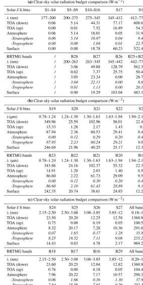
The clear-sky comparison between Solar-J and RRTMG-SW for overhead sun (SZA = 0◦) is summarized in Table 4 and Fig. 2. Table 4 lists the band-by-band radiation bud-get in W m−2, with Solar-J’s spectral bins labeled as S-bins and RRTMG’s as B bands (B16–B29 follow the same band numbers as in RRTMG’s codes). For easy comparison, sev-eral Solar-J’s spectral bins of higher resolution from the UV range are lumped together to best match the RRTMG’s bin of similar range, and vice versa with RRTMG’s B24 and B25 bins combined to compare to Solar-J’s S18 bin. The incom-ing spectral solar irradiance is slightly different for the two codes and so for easier comparison we scale each of them to a total of 1360.8 W m−2(Kopp and Lean, 2011). RRTMG-SW adopts the solar source function from Kurucz (1992), while Solar-J integrates high-resolution (0.05 nm) photon fluxes (Meier et al., 1992) by wavelength to obtain the solar irra-diance. Clear-sky summary comparisons for the other three
SZAs (21, 62, 84◦) are shown in Table 5 under clear-sky
columns.
Table 2.Spectral properties of liquid-water and ice-water clouds and stratospheric sulfate aerosols: the real and imaginary refractive indices
(nrandni), ratio of optical to geometric cross section (Q), single scattering albedo (SSA), and the asymmetry factor (g).
Bin Liquid-water cloud:re=12 µm,ρ=1.00 g cm−3 Ice-water cloud:re=48 µm,ρ=0.917 g cm−3
nr ni Q SSA g nr ni Q SSA g
S12 1.350 1.8E−08 2.054 1.0000 0.867 1.336 5.8E−09 2.021 1.0000 0.812
S13 1.349 1.5E−08 2.053 1.0000 0.869 1.333 5.4E−09 2.021 1.0000 0.812
S14 1.348 1.4E−08 2.052 1.0000 0.869 1.332 5.1E−09 2.022 1.0000 0.812
S15 1.347 1.3E−08 2.055 1.0000 0.869 1.331 4.8E−09 2.022 1.0000 0.812
S16 1.345 9.5E−09 2.057 1.0000 0.869 1.328 4.3E−09 2.023 1.0000 0.812
S17 1.340 3.4E−09 2.062 1.0000 0.869 1.321 3.0E−09 2.025 1.0000 0.812
S18 1.333 3.1E−08 2.089 1.0000 0.863 1.310 1.7E−08 2.034 1.0000 0.812
S19 1.328 2.8E−06 2.118 0.9996 0.858 1.302 1.7E−06 2.047 0.9991 0.812
S20 1.324 1.2E−05 2.144 0.9986 0.852 1.297 1.3E−05 2.055 0.9946 0.812
S21 1.321 1.6E−04 2.155 0.9851 0.854 1.293 2.4E−04 2.060 0.9246 0.812
S22 1.313 3.2E−04 2.179 0.9752 0.852 1.284 2.2E−04 2.069 0.9413 0.812
S23 1.302 9.2E−04 2.197 0.9427 0.858 1.272 1.2E−03 2.076 0.7876 0.812
S24 1.283 6.7E−04 2.220 0.9610 0.855 1.251 4.7E−04 2.083 0.9088 0.812
S25 1.239 1.0E−01 2.211 0.4979 0.970 1.125 1.0E−01 2.071 0.5107 0.812
S26 1.428 5.1E−02 2.268 0.5240 0.939 1.496 1.6E−01 2.102 0.5408 0.812
S27 1.317 2.2E−02 2.409 0.6809 0.861 1.326 2.9E−02 2.144 0.5245 0.812
Bin Strat. sulf., volc.:re=0.422 µm,ρ=1.69 g cm−3 Strat. sulf., bkgrd:re=0.130 µm,ρ=1.69 g cm−3
nr ni Q SSA g nr ni Q SSA g
S05 1.505 0.0E+00 2.612 1.0000 0.732 1.505 0.0E+00 2.966 1.0000 0.698
S06 1.505 0.0E+00 2.638 1.0000 0.728 1.505 0.0E+00 2.936 1.0000 0.698
S07 1.505 0.0E+00 2.620 1.0000 0.735 1.505 0.0E+00 2.919 1.0000 0.699
S08 1.505 0.0E+00 2.628 1.0000 0.734 1.505 0.0E+00 2.904 1.0000 0.699
S09 1.472 0.0E+00 2.604 1.0000 0.718 1.472 0.0E+00 2.435 1.0000 0.711
S10 1.469 0.0E+00 2.606 1.0000 0.710 1.469 0.0E+00 2.379 1.0000 0.711
S11 1.464 0.0E+00 2.556 1.0000 0.707 1.464 0.0E+00 2.271 1.0000 0.711
S12 1.456 0.0E+00 2.500 1.0000 0.695 1.456 0.0E+00 2.087 1.0000 0.709
S13 1.452 0.0E+00 2.474 1.0000 0.690 1.452 0.0E+00 1.998 1.0000 0.708
S14 1.451 0.0E+00 2.461 1.0000 0.686 1.451 0.0E+00 1.940 1.0000 0.706
S15 1.451 0.0E+00 2.449 1.0000 0.683 1.451 0.0E+00 1.892 1.0000 0.704
S16 1.450 0.0E+00 2.432 1.0000 0.676 1.450 0.0E+00 1.766 1.0000 0.698
S17 1.445 0.0E+00 2.475 1.0000 0.675 1.445 0.0E+00 1.432 1.0000 0.683
S18 1.431 1.7E−08 3.017 1.0000 0.723 1.431 1.7E−08 0.620 1.0000 0.593
S19 1.424 1.5E−06 2.212 1.0000 0.663 1.424 1.5E−06 0.193 1.0000 0.434
S20 1.417 8.6E−06 1.431 0.9999 0.605 1.417 8.6E−06 0.090 0.9998 0.336
S21 1.430 9.4E−05 1.173 0.9988 0.570 1.430 9.4E−05 0.065 0.9972 0.291
S22 1.422 4.7E−04 0.724 0.9910 0.511 1.422 4.7E−04 0.033 0.9782 0.225
S23 1.410 1.3E−03 0.475 0.9672 0.456 1.410 1.3E−03 0.021 0.9184 0.182
S24 1.388 2.1E−03 0.305 0.9288 0.397 1.388 2.1E−03 0.013 0.8166 0.148
S25 1.319 5.1E−02 0.253 0.3855 0.302 1.319 5.1E−02 0.040 0.0768 0.106
S26 1.366 1.7E−01 0.424 0.1714 0.214 1.366 1.7E−01 0.098 0.0219 0.074
S27 1.406 2.1E−01 0.274 0.0744 0.091 1.406 2.1E−01 0.073 0.0066 0.033
shorter-wavelength bins (S17 or B26) reflect about 20 % of the incoming radiation, but in the adjacent bin with the Chap-puis O3 band it is only about 9 %. Thus, placing the 412– 442 nm interval with the Chappuis band results in greater at-mospheric absorption and less reflection. The benefit of mov-ing the Solar-J (and Cloud-J) band edge to 442 nm should be investigated.
Table 3.The standard tropical atmosphere and the two cloud profiles implemented in both Solar-J and RRTMG-SW. Height (Z) and pressure (P) are edge values; others are layer averages.
Layer Zedge Pedge T O3 H2O Stratus cloud LWC Cirrus cloud IWC
(km) (hPa) (K) (cm−3) (kg kg−1) LWC (g m−3) re(µm) IWC (g m−3) re(µm)
58 75.25 0.020
57 59.58 0.200 232.4 1.27E+09 3.85e−06 0 0 0 0
56 54.95 0.384 242.4 1.17E+10 3.85e−06 0 0 0 0
55 51.11 0.636 259.9 2.81E+10 3.85e−06 0 0 0 0
54 47.91 0.956 268.1 5.79E+10 3.82e−06 0 0 0 0
53 45.25 1.345 266.9 1.07E+11 3.78e−06 0 0 0 0
52 42.97 1.806 263.9 1.84E+11 3.63e−06 0 0 0 0
51 40.97 2.348 259.9 3.01E+11 3.42e−06 0 0 0 0
50 39.18 2.985 255.2 4.66E+11 3.20e−06 0 0 0 0
49 37.52 3.740 250.7 6.78E+11 3.00e−06 0 0 0 0
48 35.96 4.646 245.1 9.63E+11 2.74e−06 0 0 0 0
47 34.46 5.757 240.3 1.30E+12 2.55e−06 0 0 0 0
46 32.97 7.132 237.2 1.70E+12 2.47e−06 0 0 0 0
45 31.50 8.837 234.3 2.20E+12 2.42e−06 0 0 0 0
44 30.04 10.95 231.6 2.87E+12 2.27e−06 0 0 0 0
43 28.61 13.57 228.7 3.56E+12 2.18e−06 0 0 0 0
42 27.20 16.81 225.2 4.24E+12 2.11e−06 0 0 0 0
41 25.81 20.82 221.4 4.88E+12 2.04e−06 0 0 0 0
40 24.45 25.80 216.0 4.67E+12 1.90e−06 0 0 0 0
39 23.12 31.96 211.9 4.36E+12 1.87e−06 0 0 0 0
38 21.80 39.60 211.4 3.93E+12 1.85e−06 0 0 0 0
37 20.48 49.07 209.8 3.31E+12 1.84e−06 0 0 0 0
36 19.25 60.18 205.9 2.01E+12 1.90e−06 0 0 0 0
35 18.10 73.07 202.2 1.47E+12 2.04e−06 0 0 0 0
34 17.05 87.73 196.6 1.02E+12 3.27e−06 0 0 1.10E−06 6.99
33 16.08 104.2 191.1 4.10E+11 3.49e−06 0 0 5.88E−05 17.45
32 15.17 122.6 192.1 4.06E+11 4.76e−06 0 0 1.32E−04 21.03
31 14.28 142.8 197.6 3.25E+11 9.07e−06 0 0 3.49E−04 26.29
30 13.43 165.0 203.6 3.28E+11 1.83e−05 0 0 8.40E−04 32.17
29 12.59 188.9 209.8 3.23E+11 3.54e−05 0 0 1.02E−03 33.66
28 11.78 214.6 216.6 3.45E+11 6.38e−05 0 0 1.46E−03 36.54
27 11.00 242.1 223.4 3.55E+11 1.12e−04 0 0 2.01E−03 39.31
26 10.23 271.2 230.0 3.88E+11 1.95e−04 0 0 2.19E−03 40.12
25 9.48 302.1 236.2 4.29E+11 3.21e−04 0 0 3.41E−03 44.39
24 8.76 334.6 242.4 4.66E+11 4.94e−04 0 0 1.92E−04 22.90
23 8.06 368.6 248.2 5.02E+11 7.14e−04 0 0 3.35E−04 26.03
22 7.38 403.9 253.4 5.40E+11 9.80e−04 0 0 1.85E−05 13.38
21 6.73 440.3 258.1 5.80E+11 1.31e−03 0 0 2.59E−07 5.01
20 6.10 477.5 262.2 6.21E+11 1.78e−03 0 0 8.58E−08 3.89
19 5.51 515.4 266.0 6.22E+11 2.37e−03 0 0 2.13E−07 4.79
18 4.94 553.7 269.6 6.46E+11 3.13e−03 0 0 5.98E−08 3.58
17 4.41 591.9 272.7 6.84E+11 4.02e−03 0 0 0 0
16 3.91 629.9 275.3 7.23E+11 5.14e−03 0 0 0 0
15 3.44 667.2 278.0 6.80E+11 6.31e−03 0 0 0 0
14 3.00 703.7 280.8 6.19E+11 7.49e−03 0 0 0 0
13 2.60 738.9 282.9 6.46E+11 8.67e−03 0 0 0 0
12 2.22 772.7 284.9 6.72E+11 1.00e−02 0 0 0 0
11 1.88 804.6 286.9 6.97E+11 1.17e−02 2.66E−02 9.60 0 0
10 1.57 834.6 288.6 7.20E+11 1.35e−02 2.05E−02 9.60 0 0
9 1.30 862.3 290.3 7.41E+11 1.45e−02 8.66E−02 9.60 0 0
8 1.05 887.6 291.8 6.30E+11 1.54e−02 1.21E−01 9.60 0 0
7 0.83 910.3 293.0 6.22E+11 1.62e−02 9.67E−02 9.60 0 0
6 0.64 930.3 294.2 6.34E+11 1.71e−02 4.22E−02 9.60 0 0
5 0.49 947.7 295.3 6.45E+11 1.79e−02 1.53E−02 9.60 0 0
4 0.35 962.3 296.1 6.54E+11 1.84e−02 6.62E−03 9.60 0 0
3 0.25 974.3 296.7 6.62E+11 1.89e−02 3.01E−03 9.60 0 0
2 0.10 990.9 297.7 6.69E+11 1.98e−02 5.69E−04 9.60 0 0
Table 4.Spectral shortwave radiation energy budget in W m−2under clear aerosol-free July tropical conditions: Solar-J versus RRTMG. The solar constant is set at 1360.8 W m−2. For easy comparison, some Solar-J bins are combined to best match RRTMG’s band of similar range and vice versa. Note that the atmospheric absorption is further split into the stratospheric and tropospheric components (see numbers in italics).
(a)Clear-sky solar radiation budget comparison (W m−2)
Solar-J S-bins S1–S4 S5–S9 S10–S16 S17 S18
λ(nm) 177–200 200–275 275–345 345–412 412–778
TOA (down) 0.06 5.14 44.31 77.17 608.68
TOA (up) 0.00 0.01 7.52 16.89 54.36
Atmosphere 0.06 5.14 18.01 0.05 31.96
-Stratosphere 0.06 5.14 16.97 0.04 9.41 -Troposphere 0.00 0.00 1.04 0.01 22.55
Surface 0.00 0.00 18.78 60.23 522.43
RRTMG bands / B28 B27 B26 B25+B24
λ(nm) / 200–263 263–345 345–442 442–778
TOA (down) / 3.06 49.88 128.79 562.34
TOA (up) / 0.02 7.37 25.75 50.44
Atmosphere / 3.05 23.24 0.00 28.77
-Stratosphere / 3.04 22.11 0.00 8.60 -Troposphere / 0.01 1.13 0.00 20.17
Surface / 0.00 19.29 103.04 483.13
(b)Clear-sky solar radiation budget comparison (W m−2)
Solar-J S-bins S19 S20 S21 S22 S23
λ(µm) 0.78–1.24 1.24–1.30 1.30–1.63 1.63–1.94 1.94–2.15
TOA (down) 349.96 25.59 102.96 56.01 22.40
TOA (up) 15.33 1.28 2.17 1.43 0.6
Atmosphere 87.94 2.36 60.53 29.41 9.48
-Stratosphere 0.00 0.12 0.29 0.20 0.41 -Troposphere 87.95 2.23 60.24 29.21 9.07
Surface 246.69 21.96 40.25 25.17 12.32
RRTMG bands B23 B22 B21 B20 B19
λ (µm) 0.78–1.24 1.24–1.30 1.30–1.63 1.63–1.94 1.94–2.15
TOA (down) 343.86 24.16 102.37 55.32 22.31
TOA (up) 14.91 1.20 2.03 1.40 0.57
Atmosphere 86.60 2.22 61.73 29.09 9.52
-Stratosphere 0.00 0.12 0.30 0.20 0.42 -Troposphere 86.60 2.10 61.43 28.89 9.11
Surface 242.35 20.74 38.61 24.85 12.22
(c)Clear-sky solar radiation budget comparison (W m−2)
Solar-J S-bins S24 S25 S26 S27 All bands
λ(nm) 2.15–2.50 2.50–3.08 3.08–3.85 3.85–12 0.18–12
TOA (down) 23.50 20.20 12.25 12.58 1360.80
TOA (up) 0.75 0.00 0.19 0.05 100.53
Atmosphere 8.32 20.17 7.28 10.36 291.06
-Stratosphere 0.07 1.65 0.17 1.28 35.80 -Troposphere 8.25 18.52 7.11 9.08 255.26
Surface 14.43 0.03 4.78 2.17 969.23
RRTMG bands B18 B17 B16 B29 All bands
λ(nm) 2.15–2.50 2.50–3.08 3.08–3.85 3.85–12 0.20–12
TOA (down) 23.60 20.25 12.04 12.82 1360.80
TOA (up) 0.76 0.00 0.18 0.05 104.45
Atmosphere 7.96 20.22 7.17 10.57 290.27
-Stratosphere 0.06 1.66 0.16 1.30 37.91 -Troposphere 7.84 18.56 7.01 9.26 252.36
0 5 10 15 20 25 30 35
Vertical height (km)
20 25 30 35 40 45 50 55 60 65
Solar-J (solid-dot thin lines)
RRTMG-SW (dashed thick lines) (a)
Clear-sky heating in the stratosphere
-4 -3 -2 -1 0 1 2 3 4 5
20 25 30 35 40 45 50 55
(b)
Solar-J minus RRTMG-SW (stratosphere)
K day-1
0 0.5 1 1.5 2 2.5 3 3.5
Vertical height (km)
0 2 4 6 8 10 12 14 16 18
(c)
Clear-sky heating in the troposphere
K day-1
-0.4 -0.3 -0.2 -0.1 0 0.1 0.2 0.3 0.4 0.5 2
4 6 8 10 12 14
(d)
Solar-J minus RRTMG-SW (troposphere)
SZA=0 ° SZA=21° SZA=62° SZA=84°
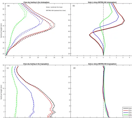
Figure 2.Aerosol-free cloudless atmospheric heating profiles of Solar-J (solid lines) and RRTMG-SW (dashed lines) and the difference, Solar-J minus RRTMG-SW, for a typical July tropical atmosphere at four solar zenith angles with Lambertian surface albedo of 0.06 (left and right sides). The plot is further split into the stratosphere and the troposphere (top and bottom rows). Note that the scale of the x-axis, K day−1, is 10 times larger for the stratosphere on the top panels.
84◦ the two models match closely. While spherical effects
may play some role in this shift, we suspect that Rayleigh scattering may contribute. The forward–backward enhance-ment in Rayleigh scattering is not represented in two-stream isotropic scattering. Thus, RRTMG – Solar-J differences will shift as the primary beam shifts from vertical to horizontal as a much greater fraction of the visible light is scattered. At low sun, the Rayleigh optical slant path along the solar beam is much greater than 1 for bin S17 and even∼1 for S18.
Figure 2 compares the vertical profiles of clear-sky heat-ing rates (K day−1) for overhead sun (SZA=0◦) with the abscissa axis scaled separately for the stratosphere and the troposphere. Both models produce similar structures with the heating maximum of ∼30 K day−1 in the stratosphere at about 45 km altitude and ∼3 K day−1 in the lower tro-posphere. The ability of Solar-J to match these structures
Table 5.Radiation budget comparison (W m−2)between Solar-J and RRTMG-SW for top of atmosphere (TOA), atmosphere, and surface across four SZAs. Also shown is the cloud radiative effect (CRE) of a typical marine stratus cloud, for which the atmospheric absorption is split into above cloud, in cloud, and below cloud, and the values are shown in italics.
SZA 0◦ 21.2◦ 62.2◦ 84.0◦
Flux (W m−2) 1360.8 1268.4 634.2 149.1
Clear-sky radiation budget (W m−2)
Solar-J RRTMG Solar-J RRTMG Solar-J RRTMG Solar-J RRTMG
TOA (up) 100.5 104.5 96.2 100.3 63.9 67.3 28.2 28.5
Atmosphere (absorbed) 291.1 290.2 276.6 275.3 166.5 164.0 56.6 54.9
Surface (absorbed) 969.2 966.1 895.7 892.8 403.8 402.9 64.3 65.6
Cloud radiative effect (CRE) of a marine stratus cloud (W m−2)
Solar-J RRTMG Solar-J RRTMG Solar-J RRTMG Solar-J RRTMG
TOA +473.4 +459.4 452.7 +441.2 +262.7 +255.8 +52.2 +50.3
Atmosphere +87.8 +88.2 +77.7 +78.2 +20.3 +18.5 −3.2 −3.3
Above cloud +21.1 +23.8 +17.7 +22.8 +11.3 +12.0 +3.0 +1.6
In cloud +77.5 +73.7 +70.5 +64.7 +16.1 +12.9 –3.9 –3.0
Below cloud –10.8 –9.3 –10.6 –9.2 –7.1 –6.4 –2.2 –1.8
Surface −561.2 −547.6 −530.4 −519.4 −282.9 −274.4 −49.1 −47.0
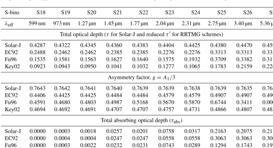
Table 6.Cirrus ice cloud optical properties: total optical depthτ for Solar-J and delta-scaledτ0for RRTMG-SW, asymmetry factorg, and absorption optical depth,τabs, for bins S18 to S27. See Table 1 for wavelength ranges and RRTMG-SW-equivalent bins.
S-bins S18 S19 S20 S21 S22 S23 S24 S25 S26 S27
λeff 599 nm 973 nm 1.27 µm 1.45 µm 1.77 µm 2.04 µm 2.31 µm 2.75 µm 3.40 µm 5.36 µm
Total optical depth (τfor Solar-J and reducedτ0for RRTMG schemes)
Solar-J 0.4287 0.4322 0.4345 0.4360 0.4383 0.4404 0.4425 0.4380 0.4470 0.4591
EC92 0.2488 0.2462 0.2462 0.2385 0.2385 0.2276 0.2276 0.3313 0.3313 0.3313
Fu96 0.1535 0.1581 0.1563 0.1627 0.1640 0.1575 0.1932 0.3709 0.3382 0.3177
Key02 0.0923 0.0943 0.0950 0.1041 0.1032 0.1277 0.1065 0.1783 0.2159 0.2266
Asymmetry factor,g=A1/3
Solar-J 0.7643 0.7642 0.7641 0.7640 0.7639 0.7639 0.7638 0.7639 0.7635 0.7631
EC92 0.4406 0.4425 0.4425 0.4484 0.4484 0.4579 0.4579 0.4907 0.4907 0.4907
Fu96 0.4591 0.4680 0.4803 0.4987 0.5168 0.5670 0.5870 0.6744 0.3411 0.0000
Key02 0.4694 0.4692 0.4691 0.4707 0.4707 0.4757 0.4731 0.4866 0.4807 0.4858
Total absorbing optical depth (τabs)
Solar-J 0.0000 0.0003 0.0018 0.0257 0.0201 0.0758 0.0317 0.2163 0.2075 0.2126
EC92 0.0000 0.0004 0.0004 0.0247 0.0247 0.0558 0.0558 0.3063 0.3063 0.3063
Fu96 0.0000 0.0003 0.0022 0.0232 0.0231 0.0743 0.0289 0.1294 0.1743 0.1972
Key02 0.0000 0.0001 0.0011 0.0178 0.0162 0.0619 0.0290 0.1491 0.1788 0.1983
stratosphere, possibly changing the stability and wave prop-agation to the high latitudes (Hsu et al., 2013). At high lat-itudes, RRTMG error is in the opposite direction, resulting in a colder polar stratosphere with possibly stronger winter vortices.
Solar-J traces the solar beam through a spherical atmo-sphere back to the sun. RRTMG assumes a flat Earth. Both
84 86 88 90 92 94
SZA (o)
J
: O
3
=
>
O
1
D
+
O
2
(
/s
)
10-6 10-5 10-4 10-3
84 86 88 90 92 94
SZA (o)
H
e
a
ti
n
g
ra
te
(
K
d
a
y
-1)
0 1 3 5
2 4
Solar-J 40 km 32 km 24 km 16 km
Solar-J RRTMG 40 km 32 km 24 km 16 km
(a) (b)
Figure 3.Ozone photolysis rates (JO3)from Solar-J(a)and the corresponding atmospheric heating rates under clear sky(b)from Solar-J (solid lines) and RRTMG-SW (dashed lines) for large solar zenith angles at four different altitudes. RRTMG-SW’s heating rates reduce to zeros at an SZA of 90◦due to the lack of sphericity correction in the plane-parallel approximation, whereas the impact of sphericity on the direct solar beam path is included in Solar-J.
heating rates from both RRTMG-SW and Solar-J. The lack of sphericity in RRTMG leads to large systematic negative biases in the heating rates at low sun. Sphericity errors ex-tend up to an SZA of 80◦but are largest of course at twilight. The high-latitude atmosphere will have SZAs greater than 80◦ for much of the day, and thus RRTMG may lead to a cold bias for the high latitudes.
3.2 Low-level marine stratus cloud
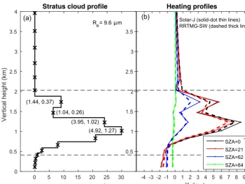
For the stratus cloud, the liquid-water path (LWP, g m−2)in each layer is derived from the LWC and height of each layer (Table 3) and is plotted versus altitude in Fig. 4a as described in Sect. 2.3. The resulting cloud optical depth in each layer, τ, (evaluated at 600 nm) is also written in pairs with Solar-J’s as the first number and RRTMG’s reduced delta-scaled optical depth (τ0) as the second. Both RRTMG and Solar-J start with same value ofτ because the Mie-based scattering phase functions for liquid water are unambiguous and both adopt the same values forre,Q, and density of liquid water. Thereis set to 9.6 µm through most of this cloud profile. The LWC increases from the surface to a maximum of 0.12 g m−3 at 1.25 km and falls to zero by 2.3 km altitude. Because of the increasing thickness of the model layers with altitude, the LWP and layerτ are not as smoothly peaked. We deem this profile realistic from comparing to the observed range for coastal marine low clouds (see Fig. 4 of Hu et al., 2007 for July liquid cloud radii distribution and Fig. 1a of Painemal et al., 2016 for LWP).
Table 5 summarizes the clear-sky radiative budget and the stratus cloud radiative effect (CRE, W m−2, calculated as change relative to clear sky) for Solar-J and RRTMG-SW for the four SZAs used here. At overhead sun (SZA=0◦) with the solar input at 1360.8 W m−2, the effect of this low-level
Liquid water path (g m )-2
0 5 10 15 20 25 30
Vertical height (km)
0 0.5 1 1.5 2 2.5 3 3.5 4
R
e= 9.6 μm
Stratus cloud profile
K day
-4 -3 -2 -1 0 1 2 3 4 5 6 7 8 9 10 0.5
1 1.5 2 2.5 3 3.5
Solar-J (solid-dot thin lines) RRTMG-SW (dashed thick lines)
Heating profiles
SZA=0 °
SZA=21°
SZA=62°
SZA=84°
(1.44, 0.37)
(1.04, 0.26)
(3.95, 1.02) (4.92, 1.27)
(b) (a)
-1
Figure 4. (a)Marine stratus cloud profile in terms of liquid-water path (LWP, g m−2)and effective radius (re, µm). The optical depth and
delta-scaled optical depth (τ,τ0)are shown in parentheses for the top five cloud layers.(b)Cloud heating profiles from Solar-J (solid lines) and RRTMG-SW (dashed lines) at four SZAs.
in RRTMG-SW. Both models show enhanced heating only in the uppermost cloud layers above 1.7 km (Fig. 4b).
We believe that the RRTMG-SW biases identified here are errors caused by the two-stream approximation. This is supported by the study of Li et al. (2015; see their Fig. 2), who show small negative errors in absorption from the cal-culation of delta-Eddington (two-stream) approximation in the case of the single-layer liquid cloud (re=10 µm,τ∼4) with cos(SZA)>0.2 (i.e., our SZAs of 0–62◦). For our SZA of 84◦, this absorption bias reverses as is also found by Li et al. (2015) for cos(SZA)<0.2. In their study, the two-stream calculations are compared to the 128-two-stream DIS-ORT (discrete–ordinate) benchmark calculations using accu-rate phase functions and no delta scaling (similar to the study of Wild et al., 2000). One other source of error in RRTMG’s model is the choice of delta-scaling factor, which they base on the HG phase function using only g. Alternatively, one can use the second moment of the true Mie phase function (Wiscombe, 1977). We revised the RRTMG-SW code to do this using Solar-J’s scattering phase functions and found a modest reduction in this error from −14 to −9 W m−2for reflected sunlight (SZA=0◦).
3.3 Tropical cirrus clouds
For the cirrus cloud comparison, we use all three ice-water parameterization options in RRTMG-SW and Solar-J’s
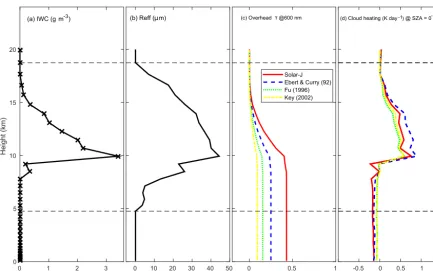
sin-gle parameterization. Figure 5a, b show the prescribed pro-files of model input of IWC andre (Table 3). The cumula-tive overhead τ at 600 nm is shown in Fig. 5c. The delta scaling varies considerably across the RRTMG parameteri-zations: Solar-J’s unscaledτ ∼0.43 compares with EC92’s τ∼0.25, Fu96’s τ ∼0.15, and Key02’sτ ∼0.09 (see also Table 6). Thus, the fraction of sunlight scattered by the cloud varies widely across all four. The asymmetry parameter g from Mishchenko’s phase functions for hexagonal and irreg-ular ice used in Solar-J ranges from 0.75 to 0.81 (as com-pared to 0.88 for equivalent-size liquid-water clouds), butg values for all RRTMG ice clouds range from 0.4 to 0.6 for wavelengths where scattering is important (S12–S24). The absorbing optical depth,τabs, is a very important diagnostic because in an optically thin cloud the overall heating should be proportional to it. Table 6 shows that all four ice cloud models have similarτabs up to S22, and if we average S23 and S24 (which appears to have been done in EC92), then all four models remain similar in terms of solar absorption. As noted for the stratus cloud, all models predict a large, fac-tor of 5, jump inτabs for S25–S27 (λ >2.5 µm), which are the most important bins for cirrus cloud heating. At these wavelengths, EC92 has the largest absorptionτabs, about 0.3, followed by Solar-J’s 0.21.
com-10-3
0 1 2 3
Height
(km)
0 5 10 15 20
(a) IWC (g m )-3
0 10 20 30 40 50 (b) Reff (μm)
0 0.5 1
(c) Overheadτ@600 nm
Solar-J Ebert & Curry (92) Fu (1996) Key (2002)
-0.5 0 0.5 1 1.5
(d) Cloud heating (K day-1) @ SZA = 0°
Figure 5. (a)Profiles of ice-water content (IWC, g m−3)and(b)effective radius (re, µm) as prescribed for both Solar-J and RRTMG-SW.
The in-cloud region, about 4–18 km, is enclosed by two horizontal dashed lines.(c)Profiles of cumulative optical depthτ at 600 nm from Solar-J and from the three RRTMG-SW parameterizations for whichτis delta scaled.(d)Cirrus cloud heating rate profiles (K day−1) at an SZA of 0◦.
ponents (reflected at top of atmosphere, absorbed in above-cloud atmosphere, in-above-cloud atmosphere, below-above-cloud atmo-sphere, and absorbed at the surface) are shown as a set of 20 bar charts in Fig. 6. The CRE percent changes relative to clear sky are shown as four color bars representing Solar-J (red), EC92 (blue), Fu96 (green), and Key02 (yellow). The clear-sky energy flux (W m−2)averaged over the four mod-els is shown in a larger font in each bar chart. For example, at an SZA of 21◦the energy absorbed by clear-sky atmosphere over the altitude range of the cirrus cloud is 98.4 W m−2. The CRE in W m−2 within the cirrus cloud for Solar-J is then 98.4×10.7 % (red bar)= +10.5. Theyaxes in Fig. 6 have different scales at different SZAs.
A key cirrus CRE is the increase in albedo, the top-of-atmosphere reflected sunlight, as shown for all models and a range of SZAs in Fig. 6 (top row). The percent increase across RRTMG-SW models (13–131 %) scales in proportion toτ, with EC92 being the largest and Key02, the smallest. This relative order stays the same across all SZAs, but the range across RRTMG-SW models decreases and the relative percent increases for larger SZAs. The Solar-J model also increases in percent with SZA, but the pattern is different from that of RRTMG-SW models. At overhead sun, Solar-J has about the same CRE percent as EC92 even though it has a 1.7 times greater τ. This can be understood in that
Solar-J cirrus is highly forward scattering and less of the scattered light is reflected backward and upward. As the SZA increases to 21–62◦, however, the peak in backscatter at 180◦becomes less important and Solar-J shifts lower relative to EC92 to look like Fu96. At very large SZA of 84◦, with most of the
sunlight being scattered at least once within the cloud, the Solar-J model again looks like the largestτ, model EC92. To first order, the Solar-J model is calculating the correct SZA dependence of the CRE by using both a more realistic scat-tering phase function and eight-stream scatscat-tering. The use of Mishchenko’s sample T-matrix phase function may not be a perfect choice for cirrus, but it is clearly more realistic than the isotropic scattering used in RRTMG-SW. Solar-J captures the cirrus albedo curve similar to Fig. 2 of Mishchenko et al. (1996) forτ=0.1 in which the slope increases rapidly as the cosine (SZA) approaches 0. While the RRTMG-SW two-stream models can be tuned to be correct at some SZAs, they will have errors of 15 W m−2 at others. The change in surface heating (fifth row) looks like the reverse of the top-of-atmosphere bars with similar relative weighting of the RRTMG-SW models. Again, it shows that two-stream scat-tering cannot mimic the correct SZA dependence of reduced surface heating under cirrus.
% 0 10 20 30 40 50
Top of atmos. (out = +)
102.6 W m-2
SZA = 0° 1361 W m-2
0 2 4 6 8 10
Above-cloud atmos. (abs = +)
36.8 % -10 -5 0 5 10
In-cloud atmos. & cloud (abs = +)
103 -20 -15 -10 -5 0
Below-cloud atmos. (abs = +)
150.8
-15 -10 -5 0
Surface (In = +)
968 0 10 20 30 40 50
98.3 W m-2
0 2 4 6 8 10 35.3 -10 -5 0 5 10 98.4 -20 -15 -10 -5 0 142.4 -15 -10 -5 0 895 0 50
100 65.7 W m
-2 0 2 4 6 8 10 23.9 -10 -5 0 5 10 62.0 -20 -15 -10 -5 0 79.7 -15 -10 -5 0 404 0 50
100 28.4 W m
-2 0 2 4 6 8 10 12.4 -50 0 50 22.0 -60 -40 -20 0 21.4 -30 -20 -10 0 65.1
SZA = 21° 1269 W m-2 SZA = 84° 149 W m-2
SZA = 62° 635 W m-2
%
%
%
Cirrus model: Solar-J E&C 92 Fu 96 Key 02
Figure 6.Percent changes (%) in shortwave radiation energy budget relative to the aerosol-free clear sky (surface albedo of 0.06) caused by a cirrus cloud using four different models: Solar-J and the three RRTMG-SW parameterizations for ice clouds. Results are shown for four different solar zenith angles. Changes in the vertical column are divided into five regions: top of atmosphere, atmospheres above, within, and below the cirrus cloud, and at the surface. Single numbers in bold shown in the corner of each panel are the clear-sky energy budget in W m−2averaged over Solar-J and RRTMG-SW for each region. Note that differenty-axis scales have been used for large SZAs.
the scattered light has only one angle, and thus the above-cloud heating (second row of Fig. 6) is strictly proportional to the top-of-atmosphere increases. With Solar-J, the reflected light is calculated at four zenith angles with the flux at larger zenith angles producing more heating (i.e., longer slant path through the atmosphere). This is most apparent in the case of the SZA of 84◦where the low-angle scattering driven by the low solar elevation produces relatively much more atmo-spheric heating.
In-cloud heating (third row) is expected to be proportional to τabs at high sun (SZA= 0–62◦), and for flux-weighted
has all models calculating 20–35 % reductions in heating be-cause of the reduced sunlight.
4 Computational costs
The major computational costs of Solar-J and similar codes within a chemistry–climate model centers on three key com-ponents: matrix operations required for multi-stream scat-tering, wavelength bins representing the spectrum of optical properties, and approximation of the multitude of indepen-dent column atmospheres (ICAs) resulting from a complex overlapping cloud field within a grid cell. What is a rea-sonable requirement for multi-stream scattering in a climate model? From this work as well as a history of publications noted above, the analytic two-stream approximation has er-rors that cannot simply be corrected or averaged over, that create large-scale biases in cloud radiative forcing with lati-tude, and that significantly misrepresent the direct–diffuse ra-tio of solar radiara-tion at the surface. The original Fast-J work (Wild et al., 2000) examined a range of multi-stream scatter-ing models and found that for typical clouds, an eight-stream solution was able to match within a few percent that of a 100-stream code for the mean intensity above, within and be-low the cloud. A major advantage of the eight-stream system was that no delta scaling was needed and a simply truncated scattering phase function could be used directly. The par-ent RRTM-SW code has the option of using a more accurate 16-stream scattering code but would in general be computa-tionally much more expensive than the eight-stream Solar-J. The basic costs of the matrix inversions (Fast-J via Feautrier, 1964) or eigenvalue solutions (RRTM via DISORT; Stamnes et al., 1988) scale asn3. For the same eight-stream solution, DISORT performs eigenvalue decomposition of 8×8 ma-trices at each level at a cost of order 83, while the Feautrier approach solves the finite-difference equations with 4×4 ma-trices at split levels for a cost of order 2×43. As a first guess, the Feautrier code should run 4 times faster than the equiv-alent DISORT code. We examine the costs and options of wavelength binning and cloud-field approximations below.
4.1 Solar-J versus RRMTG-SW
Cloud-J (and hence Fast-J) has been extensively tested in the UC Irvine chemistry-transport model (CTM). Cloud-J timings are estimated by comparing full cloud quadrature (2.75 calls per column atmosphere per time step; see be-low) versus an average-cloud approximation (1 call). We find that 12 % of the CTM wall-clock time is spent in Cloud-J using average clouds and 28 % when using cloud quadra-ture. Because the UCI CTM runs a minimalist tropospheric chemistry and a linearized stratospheric chemistry (see Hsu and Prather, 2010), it keeps track of only 32 species. More complete models like Oslo CTM3 (Søvde et al., 2012) and WACCM (Marsh et al., 2013) calculate transport and
chem-istry of about 100 species. In CTMs like these, the fractional cost of Cloud-J should be only 4–7 %. Comparing Solar-J to Cloud-J in single-atmosphere tests shows what is expected; Solar-J costs are 3.5 times greater because of the much larger number of spectral bands needed for heating (100 versus 18). A minor feature is that cloudy atmospheres cost about 10 % more than clear atmospheres because Cloud-J inserts extra layers at the top of clouds to enhance the accuracy of the finite-difference equations.
In a series of comparisons on a single-socket multi-threaded CPU, we find that Solar-J takes 5 times more wall clock time than RRTMG-SW. This is not surprising given the cost of solving an eight-stream versus two-stream RT problem. An additional cost of Solar-J (not included above) is spherical geometry. With RRTMG-SW, 50 % of the grid cells are in sunlight and require RT solutions. With Solar-J, however, important photochemistry and solar heating occur in the atmosphere when the surface is past sunset (see Fig. 3) involving about 56 % of the grid cells, a 12 % increase in radiatively active grid cells. One could expect that RRTMG-SW will correct this error and end up with similar increases in coverage and cost.
Most climate models, even at the highest resolutions, have individual grid cells with fractional, overlapping cloud lay-ers. Although 3-D RT models can be used to solve for the average heating and photolysis rates, most climate mod-els decompose the cloud structures into ICAs, for example, through cloud-resolving models (Khairoutdinov et al., 2005) or from cloud fractional coverage and a decorrelation dis-tance for overlapping cloud layers (Prather, 2015). The ICAs are horizontally homogeneous and can be solved using the 1-D RT codes of RRTMG-SW or Solar-J. Comparisons be-tween Solar-J and RRTMG-SW for clouds in Sect. 3 are done with a single 1-D plane-parallel, ICA-like atmosphere (i.e., 100 % cloud fraction in each cloud layer), an idealized case. Although the different approaches for fractional cloud cover were not directly tested here, it is worth looking at how Solar-J and RRTMG might treat cloud fields in cli-mate models. The Monte Carlo ICA (McICA; Pincus et al., 2003) method selects both ICAs and spectral intervals ran-domly in each grid square. Every spectral interval is sampled only once, and each may have a different ICA selected ac-cording to its fractional area (frequency of occurrence). With 100+ bin–ICA combinations, the ICAs are well sampled, but there may be instances in which a few key large-energy bins are not sampled accurately. The McICA approach, when suitably averaged over time, has no mean bias in average heating rates but very large root mean square (rms) errors: e.g., ±105 W m−2 in surface heating with an SZA of 45◦;
cir-rus clouds, typical stratus clouds, and very thick frontal or cumulus clouds. While each grid cell may have up to four QCAs, on average there are only 2.75. Solar-J then calcu-lates all wavelength bins using all QCAs to compute the average. Cloud-J (Prather 2015) compared several approxi-mations for calculating average photolysis rates (Js) within a sample of 640 tropical atmospheres where the generated number of ICAs per grid cell ranged from 1 to 3500 and av-eraged 170. Compared to the exact answer defined by sepa-rate calculations with all the weighted ICAs, cloud quadra-ture achieves rms errors in instantaneous cell-averaged Js of 0 to 3 % throughout the troposphere, with most levels being 0–1 %. When Cloud-J is run selecting random ICAs (using all wavelengths for each ICA, not the McICA approach), 50 random ICAs (18 times greater cost) are needed to achieve the accuracy of cloud quadrature.
From the point of view of chemistry–climate models, large rms errors in Js cannot be tolerated because the chemistry is non-linear and such errors are not likely to average. In cli-mate models, there are threshold processes like aerosol and ozone heating preventing cloud formation (e.g., Koch and DelGenio, 2010), for which heating noise may not simply av-erage out. Errors in heating rates do not always have symmet-ric responses in terms of climate (e.g., Hsu et al., 2013). Al-though Pincus et al. (2003) tested climate forecasting with an early version of McICA, it is not clear how forecast skill with modern, high-resolution models is impacted by the biases in RRTMG-SW. Alternatively, RRTMG-SW could adopt cloud quadrature with 2.8 times greater cost and eliminate most of their rms errors in heating.
All of these standard features of Solar-J (eight streams, spherical geometry, cloud quadrature) increase the computa-tional cost, but one can argue that the improved fidelity in the solar heating of the atmosphere and radiative forcing of the climate is worth the cost. The question is what fraction of the total computational cost of a climate simulation would be used by Solar-J. If we estimate the fractional cost of RRTMG in a full atmosphere–ocean climate simulation to be 1–3 %, then replacing it with Solar-J (5 times greater) and includ-ing cloud quadrature (2.8 times greater), would increase this to 13–39 %. At the lower end of this range, the substantially improved and less noisy physics is probably worth it, but at the upper end it is prohibitive. In either case, it is worthwhile to pursue a range of computer science and algorithmic ap-proaches to reduce these costs as discussed in Sect. 4.2 and 4.3 below.
4.2 Computer science options
A profiling of the Solar-J code shows that the Fast-J core, consisting of a scattering matrix generator and block-tridiagonal solver, is the dominant cost. These two subrou-tines are already well optimized in terms of single CPU multi-threading; however, porting Fast-J to computers with graphical processing units (GPUs) has shown promise for
greater speed. One effort targeted a single GPU and demon-strated speedups via CUDA (Compute Unified Device Archi-tecture) tuning of∼50 times more relative to the CPU time if a large number of column atmospheres (200+)were con-currently evaluated (Artico et al., 2015). Another effort used a field-programmable gate array (FPGA) with the advantage that it applies to a single column calculation. The FPGA re-sulted in a∼4 times greater speedup and a rather dramatic 35 times more energy savings compared to the multicore pro-cessor computation (Rezaei et al., 2016). Fast-J was also op-timized for the Xeon Phi on the Babbage test platform at DOE National Energy Research Scientific Computing Center (NERSC) and achieved∼3 times faster speedups with only a subset of the cores.
Great computational acceleration could be realized with GPU systems when a number of column atmospheres are be-ing simultaneously evaluated. For each grid cell, Solar-J cal-culates about 100 wavelength bins and an average of 2.75 ICAs per grid square. Giving each CPU/GPU node a 3×3 grid cell square (∼2500 column atmospheres) could achieve 10 times greater or faster speedups for Solar-J and be ap-propriate for a massively parallel climate simulation (e.g., 32 000 nodes for a 50 km global grid). With such speedups, Solar-J costs would be comparable or possibly less than those of the current RRTMG-SW and thus become a marginal cost in the climate simulation.
4.3 Other parameterizations for wavelength bins
Solar-J uses its own optimization of wavelength bins at ultra-violet and visible wavelengths (0.18 to 0.8 µm), which is based on previously established experience with O2and O3 cross sections and the need to calculate accurate J values. We accept that RRTMG-SW and its parent code RRTM rep-resent current best practice and accuracy in characterizing the absorption of infrared sunlight (0.8 to 12 µm) in the Earth’s atmosphere and have adopted the RRTMG-SW code exactly for bins and all gaseous absorbers. Solar-J’s compu-tational cost is clearly driven by the additional 82 infrared bins adopted from RRTMG-SW. Alternative methods of pa-rameterizing these infrared bins need to be examined: e.g., 14 bins (Chou, 1992; Grant and Grossman, 1998), 34 bins (Fu and Liou, 1992), and 36 bins (Cole, 2005). Any of these would result in 1.5–2.5 times more savings for Solar-J. We recognize that the infrared bins adopted in RRTMG-SW are based on accurate representation of the line-by-line calcula-tions, and thus adopting these reduced-bin parameterizations will introduce new errors, but further research will be needed to determine whether these errors maybe an acceptable trade-off for speed gain.
their importance in tropospheric heating rates. For our clear-sky case here (Table 4, Fig. 2), we find an average tropo-spheric heating rate of 2.4 K day−1. The contribution of CH
4 to this total is 0.1 %; that of CO2is complex because of the stratospheric self-shielding but is less than±1 % in the tro-posphere, and that of O2is about 3 % uniformly throughout the troposphere. If we can find a way of treating the O2 heat-ing separately, then the effort to find an abbreviated number of spectral intervals can focus on water vapor.
5 Conclusions
We present a new solar radiation module. Solar-J version 7.5 aims for consistent calculation of atmospheric photolysis and solar heating rates by combining the strengths of both Cloud-J and RRTMG-SW. In a chemistry–climate model, Solar-Cloud-J supplies the needs of solar heating of the atmosphere and surface, photolysis rates, and photosynthetic activity. Cli-mate models are increasingly including short-lived gases and aerosols as radiative forcing components, and the accurate simulation of these under different climates requires some level of interactive chemistry and photolysis rates.
The components of Solar-J are chosen and balanced to achieve the best possible overall accuracy for a module in-tended as a standard component of chemistry–climate sim-ulations. From Cloud-J, we take the eight-stream scatter-ing model, semi-spherical geometry, ultraviolet transmission, and cloud quadrature. From RRTMG-SW, we take the de-tailed spectral intervals for the visible and infrared developed from the RRTM reference code. Solar-J matches RRTMG-SW except where the improved physics leads to more accu-rate results. Selecting the best physics for all these compo-nents comes with a cost: a simple comparison shows the cost of Solar-J is 5 times that of RRTMG-SW for a single atmo-sphere, and if the cloud quadrature scheme for overlapping cloud fields (Neu et al., 2007; Prather, 2015) is applied to ei-ther code, the cost increases additionally by 2.8 times. We show that Solar-J can be optimized on GPUs and achieve speeds similar to RRTMG-SW. While this opens up great opportunities for the new generation of high-performance computers, it also complicates the simple implementation of Solar-J in a climate model.
J is a starting point. In assessing the fidelity of Solar-J in terms of interaction with the many components of the climate system, we can focus on the three major sources of costs/error (spectral intervals, multi-stream radiative transfer, and complex cloud systems) and, in parallel, on the opportu-nities for accelerated performance with new computational architectures. Ideally, the community would optimize com-putational costs across modules to have comparable (small) errors in all. In addition, these parameterization errors need to be evaluated for the impact they might have on climate simulations (e.g., Pincus et al., 2003). For Solar-J, the next steps consist of (i) moving the S17–S18 boundary to the
be-ginning of the O3Chappuis absorption near 0.5 µm, and (ii) developing a more realistic and diverse range of cirrus clouds and their optical properties (e.g., Yang et al., 2015). An-other inquiry is to test some of the published, simpler models for water vapor absorption against RRTMG-SW. A larger project will be to put Solar-J into a climate model and eval-uate how errors in modeling solar radiation may affect the climate simulations.
Code availability. The most recent version of Solar-J can be found at ftp://128.200.14.8/public/junoh/Solar-J/. A complete version of Solar-J code and data, along with some stand-alone test cases, is included in a zip file as a Supplement to this article.
The Supplement related to this article is available online at https://doi.org/10.5194/gmd-10-2525-2017-supplement.
Competing interests. The authors declare that they have no conflict of interest.
Acknowledgements. This work is supported by the US Department
of Energy, Office of Science, Biological and Environmental Research Program under award nos. SC0007021 and DE-SC0012536, and by NASA Modeling, Analysis and Prediction (MAP) program under award no. NNX13AL12G. This research used resources of the National Energy Research Scientific Com-puting Center, a DOE Office of Science User Facility supported by the Office of Science of the US Department of Energy un-der contract no. DE-AC02-05CH11231. Part of this work was performed under the auspices of the US Department of Energy by Lawrence Livermore National Laboratory under contract no. DE-AC52-07NA27344.
Edited by: Gerd A. Folberth
Reviewed by: two anonymous referees
References
Artico, F., Prather, M. J., Veidenbaum, A. V., and Nicolau, A.: Fast Fast-J GPU Codes, CECS technical report, 15-03, 8 November 2015.
Barker, H. W., Cole, J. N. S., Li, J., Yi, B., and Yang, P.: Estimation of Errors in Two-Stream Approximations of the Solar Radiative Transfer Equation for Cloudy-Sky Conditions, J. Atmos. Sci., 72, 4053–4074, https://doi.org/10.1175/JAS-D-15-0033.1, 2015. Beyer, K. D., Ravishankara, A. R., and Lovejoy, E. R.:
Measure-ments of UV refractive indices and densities of H2SO4/H2O and
H2SO4/HNO3/H2O solutions, J. Geophys. Res.-Atmos., 101,
14519–14524, https://doi.org/10.1029/96JD00937, 1996. Bian, H. and Prather, M. J.: Fast-J2: Accurate Simulation of