ISSN: 1821-1291, URL: http://www.bmathaa.org Volume 9 Issue 4(2017), Pages 31-41.
ON THE GLOBAL STABILITY OF A NEUTRAL DIFFERENTIAL EQUATION WITH VARIABLE TIME-LAGS
YENER ALTUN, CEMIL TUNC¸
Abstract. In this work, we get assumptions that guaranteeing the global ex-ponential stability (GES) of the zero solution of a neutral differential equation (NDE) with time-lags. By help of the Liapunov-Krasovskii functional (LKF) approach, we obtain a new result related (GES) of the zero solution of the studied (NDE). An example is given to illustrate the applicability and cor-rectness of the obtained result by MATLAB-Simulink. The obtained result includes and improves the results found in the literature.
1. Introduction
In 2014, Keadnarmol and Rojsiraphisal [10] considered the first order neutral differential equation (NDE) with two variable time-lags,
d
dt[x+px(t−τ(t))] =−ax+btanhx(t−σ(t)). (1.1)
Using Lyapunov functionals, the authors established some sufficient conditions for the (GES) of solutions of (NDE) (1.1). By this work, the authors [10] established an improved criterion for the (GES) of solutions of (NDE) (1.1). In this paper, instead of (NDE) (1.1), we consider the first order non-linear (NDE) with two variable time-lags:
d
dt[x+p(t)x(t−τ(t)] =−a(t)h(x)−b(t)g(x(t−τ(t)))
+c(t) tanhx(t−σ(t)), t≥0, (1.2)
where ”′” represents d
dt, a, b, c, p : [t0,∞) → [0,∞), t0 ≥ 0, and g, h : ℜ → ℜ are continuous functions with g(0) = 0, h(0) = 0; the function c is continuous and differentiable, and |p(t)| ≤ p0 < 1 ( p0-constant). The variable time-lags τ and σ are continuous and differentiable, defined by τ(t) : [0,∞) → [0, τ0] and
σ(t) : [0,∞)→[0, σ0] satisfying
0≤τ(t)≤τ0, 0≤σ(t)≤σ0,
τ′(t)≤δ1, σ′(t)≤δ2<1, (1.3) whereτ0>0, σ0>0, δ1>0, δ2(>0)∈ ℜ.
2000Mathematics Subject Classification. 34K20, 34K40, 47N20.
Key words and phrases. (NDE); (GES); (LKF); matrix inequality; multiple time-lags. c
2017 Universiteti i Prishtin¨es, Prishtin¨e, Kosov¨e.
Submitted September 30, 2017. Published October 30, 2017. Communicated by Tongxing Li.
Throughout the paper, we assume that assumptions given by (1.3) hold when we needxshowsx(t).
For (NDE) (1.2), we assume the existence initial condition
x0(θ) =φ(θ), θ∈[−r,0],
wherer= max{τ0, σ0},φ∈C([−r,0];ℜ). Define
h1(x) =
h(x) x , x6= 0
dh(0) dt , x= 0
(1.4)
and
g1(x) =
g(x) x , x6= 0
dg(0) dt , x= 0.
(1.5)
It is seen from (NDE) (1.2) and (1.4), (1.5) that
d
dt[x+p(t)x(t−τ(t))] =−a(t)h1(x)x−b(t)g1(x(t−τ(t)))x(t−τ(t))
+c(t) tanhx(t−σ(t)). (1.6)
In this paper, we discuss the (GES) of the zero solution of (NDE) (1.2). Meanwhile, it is well known that (NDEs) without or with time-lags often occur in many scientific areas such as engineering techniques fields, physics, medicine and etc. (see [1-29] and the references therein). Therefore, it is worth investigating the (GES) of (NDE) (1.2). In the relevant literature, the most of researchers have focused on the qualitative properties of special case of (NDEs) (1.1) and (1.2) with constant coefficients and constant time-lags like
d
dt[x+px(t−τ)] =−ax+btanhx(t−σ) (1.7)
or its different models. During the investigations, the authors benefited from differ-ent methods such as the Liapunovs function (direct) method, Liapunov-Krasovskii functional (LKF) method, integral inequalities, LMI, perturbation techniques, model transformations, etc., to obtain specific conditions on the various qualitative proper-ties of (NDEs) (see [1-29]). It is also worth mentioning that this paper especially mo-tivated by the results of Keadnarmol and Rojsiraphisal [10] and those can be found in the references of this paper. When we consider (NDEs) (1.1), (1.2) and (1.7) and compare our equation, (NDE) (1.2) with that discussed by Keadnarmol and Rojsiraphisal [10], (NDE) (1.1), it follows that (NDE) (1.2) includes and improves (NDE) (1.1). In fact, if we choose p(t) = p is a constant, a(t)h(x) = ax, a >0,
2. Preliminaries
For convenience, let D1(t) = x+p(t)x(t−τ(t)). Hence, (NDE) (1.6) can be written as
D′1=
d
dt[x+p(t)x(t−τ(t))] =−a(t)h1(x)x
−b(t)g1(x(t−τ(t)))x(t−τ(t)) +c(t) tanhx(t−σ(t)).
Therefore, we have
D′
1=−a(t)h1(x)x−b(t)g1(x(t−τ(t)))x(t−τ(t)) +c(t) tanhx(t−σ(t)) 0 =−D1+x+p(t)x(t−τ(t)). (2.1)
Definition 1. The solutionx= 0 of (NDE)(1.6) is (ES) if
kxk ≤Kexp(−λt) sup
−r≤s≤0
kx(s)k=Kexp(−λt)kx0ks, (2.2)
whereK(>0)∈ ℜ,λ(>0)∈ ℜ, andkxtks= sup−r≤s≤0kx(t+s)k.
Lemma 2. Let N ∈ ℜn×n be any symmetric and positive definite matrix and x, y∈ ℜn. Then
±2xTy≤xTN x+yTN−1y.
Proposition 3. Let M > 0, µ > 0, |p(t)| ≤ p0 < 1, and 0 ≤ τ(t) ≤ τ0. If
x: [−τ0,∞)→ ℜsatisfies kxk ≤ sup
s∈[−τ0,0]
kx(s)k=kx0ks, t∈[−τ0,0]
and
kxk ≤p0kx(t−τ(t))k+Mexp(−µt),
then there are positive constantsε, m∈[0,−lnp0
τ0 ] such that p0exp(ετ0)<1
and
kxk ≤ kx0ksexp(−mt) +
M
1−p0exp(ετ0)
exp(−εt)≤Nexp(−ϑt), (2.3)
wheret≥0, N =kx0ks+1−p0exp(M ετ0) andϑ= min{m, ε}.
Proof. In view of the assumptions|p(t)| ≤p0<1 and 0≤τ(t)≤τ0 one can find sufficient small positive constant ε, m ∈ [0,−lnp0
τ0 ] such that p0exp(ετ0) < 1 and p0exp(mτ0)<1. We verify that inequality (2.3) is true. If µ≤ε, we can choose
µ=ε; else ifµ > ε, we have exp(−µt)≤exp(−εt). Lett= 0. Hence we have
kx(0)k ≤p0kx(−τ(0))k+M ≤p0 sup
−τ0≤s≤0
kx(s)k+M
<kx0ks+
M
1−p0exp(ετ0) ≡N.
Therefore, estimate (2.3) is true whent= 0.
Now, lett > 0. Assume that inequality (2.3) fails. Then, there is t∗ >0 such
that
kx(t∗)k>kx0ksexp(−mt∗) +
M
1−p0exp(ετ0)exp(−
and
kx(t)k ≤ kx0ksexp(−mt)+
M
1−p0exp(ετ0)
exp(−εt)≡Nexp(−ϑt)f or all t∈[0, t∗).
I.Lett∗> τ(t∗)>0. Then,
kx(t∗)k ≤p0kx(t∗−τ(t∗))k+Mexp(−µt∗)
≤p0{kx0ksexp(−m(t∗−τ(t∗))) +
M
1−p0exp(ετ0)
exp(−ε(t∗−τ(t∗)))}
+Mexp(−εt∗)
≤p0exp(mτ0)kx0ksexp(−mt∗) +
M p0exp(ετ0) 1−p0exp(ετ0)
exp(−εt∗)
+Mexp(−εt∗)
≤ kx0ksexp(−mt∗) +
M
1−p0exp(ετ0)exp(−
εt∗)≡Nexp(−ϑt∗).
II.Let−τ0<0< t∗< τ(t∗). Then kx(t∗−τ(t∗))k ≤ kx0k
s= sup s∈[−τ0,0]
kx(s)k,
and hence, it follows that
kx(t∗)k ≤p0kx(t∗−τ(t∗)k+Mexp(−µt∗)
≤ kx0ksexp(−mt∗) +
M
1−p0exp(ετ0)
exp(−εt∗)
≡Nexp(−ϑt∗).
Thus, for both the cases I and II, we have a contradiction to inequality (2.4). Therefore, inequality (2.3) is true for allt≥0.
3. Exponential stability
We assume that there exist nonnegative ai, bi, mi, ni and positive constants ci,(i= 1,2),such that fort≥t0,
a1≤a(t)≤a2, b1≤b(t)≤b2, c1≤c(t)≤c2, c′(t)≤0, (3.1)
m1≤g1(x)≤m2, n1≤h1(x)≤n2. (3.2)
Theorem 4. Letai, bi, mi, ni be nonnegative constants and estimate (1.3) holds. Then trivial solution of (NDE) (1.6) is (GES) if the operatorD1is stable (i.e.|p(t)| ≤
p0 < 1) and there exist positive constants c1, c2, q1, α, k and constants qi,(i = 2,3, ...,6), such that
Ω =
2kq1−2q2 (1,2) (1,3) q1c2 q3 ∗ (2,2) (2,3) 0 q5+ 2q6 ∗ ∗ (3,3) 0 −2q6 ∗ ∗ ∗ −c1(1−δ2) 0
∗ ∗ ∗ ∗ −2q6
<0, (3.3)
matrix Ω.
Proof. We define a (LKF)V =V1+V2+V3=V1(t) +V2(t) +V3(t) by
V1(t) =e2kt[D1, x,0]
1 0 0 0 0 0 0 0 0
q1 0 0
q2 q3 0
q4 q5 q6
D1 x 0
=e
2ktq 1D12,
V2(t) =α
Z t
t−τ(t)
e2k(s+τ0)
x2(s)ds+c(t)
Z t
t−σ(t)
e2k(s+σ0)tan
h2x(s)ds,
V3(t) =ηe2ktD21,
where D1 =x+p(t)x(t−τ(t)), q1 > 0, α > 0, c(t) >0, qi ∈ ℜ,(i = 2, ...,6), and η(>0)∈ ℜ, we determine it later.
DifferentiatingV1 andV2along system (2.1), we get
V′
1(t) =e2kt(2kq1D12+ 2q1D1D′1)
= 2e2ktkq1D21+ 2e2kt[D1, x,0]
1 0 0 0 0 0 0 0 0
q1 q2 q3 0 q4 q5 0 0 q6
D′ 1 0 0 .
Benefited from the formula,x−x(t−τ(t)) =Rt
t−τ(t)x
′(s)ds, we obtain
V1′(t) = 2e2ktkq1D12
+ 2e2kt[D1, x,−
Z t
t−τ(t)
x′(s)ds+x−x(t−τ(t))]
q1 q2 q3 0 q4 q5 0 0 q6
×
−a(t)h1(x)x−b(t)g1(x(t−τ(t)))x(t−τ(t)) +c(t) tanhx(t−σ(t)) −D1+x+p(t)x(t−τ(t))
Rt
t−τ(t)x
′(s)ds−x+x(t−τ(t))
= 2e2ktkq 1D12
+ 2e2kt[D1q1, D1q2+q4x, D1q3+q5x−q6
Z t
t−τ(t)
x′(s)ds+q6x−q6x(t−τ(t))]
×
−a(t)h1(x)x−b(t)g1(x(t−τ(t)))x(t−τ(t)) +c(t) tanhx(t−σ(t)) −D1+x+p(t)x(t−τ(t))
Rt
t−τ(t)x
′(
s)ds−x+x(t−τ(t))
= 2e2ktkq1D12+ 2e2kt{−D1q1a(t)h1(x)x
−D1q1b(t)g1(x(t−τ(t)))x(t−τ(t)) +D1q1c(t) tanhx(t−σ(t)) −D21q2+D1q2x+D1q2p(t)x(t−τ(t))
−D1q4x+q4x2+q4p(t)xx(t−τ(t))
+D1q3
Z t
t−τ(t)
x′(s)ds−D
1q3x+D1q3x(t−τ(t))
+q5x
Z t
t−τ(t)
x′(s)ds−q5x2+q5xx(t−τ(t))
−q6[
Z t
t−τ(t)
x′(s)ds]2+q6x
Z t
t−τ(t)
x′(s)ds−q6x(t−τ(t))
Z t
t−τ(t)
+q6x
Z t
t−τ(t)
x′(s)ds−q
6x2+q6xx(t−τ(t))
−q6x(t−τ(t))
Z t
t−τ(t)
x′(s)ds+q6xx(t−τ(t))−q6x2(t−τ(t))}
=e2kt{(2kq
1−2q2)D21+ 2[−q1a(t)h1(x) +q2−q3−q4]xD1 + (2q4−2q5−2q6)x2+ 2D1q1c(t) tanhx(t−σ(t))
+ 2[−q1b(t)g1(x(t−τ(t))) +q2p(t) +q3]x(t−τ(t))D1
+ 2(q4p(t) +q5+ 2q6)xx(t−τ(t)) + 2D1q3
Z t
t−τ(t)
x′(s)ds
−2q6x2(t−τ(t))−4q6x(t−τ(t))
Z t
t−τ(t)
x′(s)ds
+ 2(q5+ 2q6)x
Z t
t−τ(t)
x′(s)ds−2q6[
Z t
t−τ(t)
x′(s)ds]2}.
Using conditions (3.1), (3.2) and|p(t)| ≤p0<1, we have
V1′(t)≤e2kt{(2kq1−2q2)D12+ 2(−q1a1n1+q2−q3−q4)xD1 + 2(q4−q5−q6)x2+ 2q1c2D1tanhx(t−σ(t))
+ 2(−q1b1m1+q2p0+q3)D1x(t−τ(t)) + 2(q4p0+q5+ 2q6)xx(t−τ(t))
+ 2q3D1
Z t
t−τ(t)
x′(s)ds−2q6x2(t−τ(t))−4q6x(t−τ(t))
Z t
t−τ(t)
x′(s)ds
+ 2(q5+ 2q6)x
Z t
t−τ(t)
x′(s)ds−2q6[
Z t
t−τ(t)
x′(s)ds]2}, (3.4)
V2′(t)≤αe2k(t+τ
0)
x2−αe2k(t+τ0−τ(t))
(1−τ′(t))x2((t−τ(t))
+c′(t)
Z t
t−σ(t)
e2k(s+σ0)tan
h2x(s)ds+c(t)e2k(t+σ0)tan h2x
−c(t)e2k(t+σ0−σ(t))(1−
σ′(t)) tanh2x(t−σ(t)).
Using conditions (1.3), (3.1) and applying the estimate tanh2x≤x2, we obtain
V′
2(t)≤e2kt{(αe2kτ
0
+c2e2kσ0)x2−α(1−δ1)x2(t−τ(t))
−c1(1−δ2) tanh2x(t−σ(t))}. (3.5)
Combining equations (3.4) and (3.5), we have
V1′(t) +V2′(t)≤e2kt{(2kq1−2q2)D21
+ 2(−q1a1n1+q2−q3−q4)xD1
+ 2(−q1b1m1+q2p0+q3)D1x(t−τ(t)) + 2(q4p0+q5+ 2q6)xx(t−τ(t))
+ 2q3D1
Z t
t−τ(t)
x′(s)ds+ 2(q5+ 2q6)x
Z t
t−τ(t)
x′(s)ds
+ [−2q6−α(1−δ1)]x2(t−τ(t))−4q6x(t−τ(t))
Z t
t−τ(t)
x′(s)ds
−c1(1−δ2) tanh2x(t−σ(t))−2q6[
Z t
t−τ(t)
x′(s)ds]2}
=e2ktlT(t)Ωl(t)
where l(t) = [D1, x, x(t−τ(t)),tanhx(t−σ(t)),Rtt−τ(t)x′(s)ds]T and Ω is defined by (3.3). Making use of assumption Ω<0, we have
V1′(t) +V2′(t)≤e2ktlT(t)Ωl(t)<0.
Therefore, there is a constantλ, λ >0, such that
V1′(t) +V2′(t)≤ −λe2kt
kD1k2+kxk2+kx(t−τ(t)k2
+ktanhx(t−σ(t))k2+kZ t
t−τ(t)
x′(s)dsk2
≤ −λe2ktkx(t)k2.
Calculating the derivate ofV3 along system (2.1), we have
V′
3(t) = 2e2ktη(D1D′1+kD12)
= 2e2ktη{[x+p(t)x(t−τ(t))]×[−a(t)h1(x)x
−b(t)g1(x(t−τ(t)))x(t−τ(t)) +c(t) tanhx(t−σ(t))] +k[x+p(t)x(t−τ(t))]2}
= 2e2ktη{−a(t)h1(x)x2−b(t)g1(x(t−τ(t)))xx(t−τ(t)) +c(t)xtanhx(t−σ(t))−a(t)h1(x)p(t)xx(t−τ(t)) −b(t)g1(x(t−τ(t)))p(t)x2(t−τ(t))
+c(t)p(t)x(t−τ(t)) tanhx(t−σ(t))
+kx2+ 2kp(t)xx(t−τ(t)) +kp2(t)x2(t−τ(t))}.
Utilizing conditions (3.1), (3.2) and|p(t)| ≤p0<1, we have
V′
3(t)≤e2ktη{−2a1n1x2−2b1m1xx(t−τ(t)) + 2c2xtanhx(t−σ(t))−2a1n1p0xx(t−τ(t))
−2b1m1p0x2(t−τ(t)) + 2c2p0x(t−τ(t)) tanhx(t−σ(t)) + 2kx2+ 4kp0xx(t−τ(t)) + 2p20kx2(t−τ(t))}.
By means of Lemma 2, we find
Let us choose the constantη as
η =
( λ
2min{ 1 ξ,
1
2} if ψ≤0, λ
2min{ 1 ξ,
1 ψ 1
2}if ψ >0, where
ξ=−2b1m1p0+ 2p02k+|c2p0|2+ 3 andψ= 2k−2a1n1+|b1m1|2+ 4|p0k|2+|c2|2+ |a1n1p0|2.
Hence, we can obtain
V1′(t) +V2′(t) +V3′(t)≤ −λ 2e
2ktkx(t)k2<0.
Since V′(t) is negative definite and 0≤ τ(t) ≤τ0, 0 ≤ σ(t) ≤ σ
0 then, V(x) ≤
V(x(0)) for allt≥0, with
V(x(0)) =V1(x(0)) +V2(x(0)) +V3(x(0)) =q1[x(0) +p(0)x(−τ(0))]2
+α
Z 0
−τ(0)
e2k(s+τ0)
x2(s)ds+c(0)
Z 0
−σ(0)
e2k(s+σ0)
tanh2x(s)ds
+η[x(0) +p(0)x(−τ(0))]2
≤q1(1 +p0)2kx0k2 s+α
Z 0
−τ(0)
e2k(s+τ0)( sup −r≤s≤0
kx(s)k)2ds
+c2
Z 0
−σ(0)
e2k(s+σ0)
( sup
−r≤s≤0
kx(s)k)2ds+η(1 +p0)2kx0k2s
≤q1(1 +p0)2kx0k2s+αe2kτ 0
τ0kx0k2s+c2e2kσ0σ0kx0k2s+η((1 +p0)2kx0k2s = ∆kx0k2
s
where ∆ =q1(1 +p0)2+αe2kτ0τ
0+c2e2kσ0σ0+η((1 +p0)2. Fromηe2ktkD1k2≤V(x)≤∆kx0k2
s, we obtainkD1k ≤M e−kt, whereM =q∆
ηkx0ks. Because ofD1=x+p(t)x(t−τ(t)), we have
kxk=kD1−p(t)x(t−τ(t))k ≤ kD1k+kp(t)x(t−τ(t))k ≤M e−kt+p0kx(t−τ(t))k.
Since |p(t)| ≤ p0 <1 and 0≤τ(t)≤τ0, we can choose sufficiently small positive constantϑ=k < −lnp0
τ0 so thatp0e
ϑτ0 <1. Utilizing Proposition 3, we have
kxk ≤(kx0ks+ M
1−p0eϑτ0)e
−ϑt, t≥0.
Choosingγ= max{kx0ks,1−pM0eϑτ0}, we obtain
kxk ≤2γe−ϑt.
This implies that the zero solution of (NDE) (1.6) is (ES). By radially unbounded-ness, it is also (GES) with rate of convergencek=ϑ >0.
uniformly asymptotically stable when the following criterion holds: Ω =
−2q2 (1,2) (1,3) q1c2 q3 ∗ (2,2) (2,3) 0 q5+ 2q6 ∗ ∗ (3,3) 0 −2q6 ∗ ∗ ∗ −c1(1−δ2) 0
∗ ∗ ∗ ∗ −2q6
<0, (3.6)
where (1,2) = −q1a1n1 +q2 −q3−q4, (1,3) = −q1b1m1+q2p0 +q3, (2,2) = 2q4−2q5−2q6+α+c2, (2,3) =q4p0+q5+ 2q6 and (3,3) =−2q6−α(1−δ1).
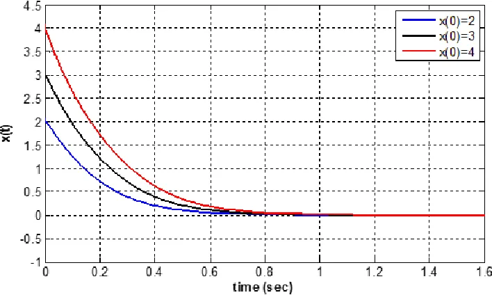
Example 1 As a special case of (NDE) (1.2), we consider the following nonlin-ear (NDE) with variable time- lags,
d dt
x+ 1
8 +t2x(t−τ(t))
=−(2 + exp(−t))
x+ x
1 +x2
−
1
2 + exp(−t)
x(t−τ(t)) + x(t−τ(t)) 1 +x2(t−τ(t))
+1
3tanhx(t−σ(t)), t≥0. (3.7)
Here,
D1(t) =x+ 1
8 +t2x(t−τ(t)), p(t) = 1 8 +t2
a(t) = 2 + exp(−t), b(t) = 1
2 + exp(−t), c(t) = 1 3
τ(t) =σ(t) = sin 2
t
20 , τ
′(
t) =sin 2t 20 <1
h(x) =x+ x
1 +x2, h1(x) =
1 + 1
1+x2, x6= 0 h′(0), x= 0
g(x) =x+ x
1 +x2, g1(x) =
1 + 1
1+x2, x6= 0 g′(0), x= 0 .
Then, we have
h(0) = 0, n1= 1≤h1(x)≤2 =n2
g(0) = 0, m1= 1≤g1(x)≤2 =m2
a1= 2≤a(t) = 2 + exp(−t)≤3 =a2
b1= 1
2 ≤b(t) = 1
2 + exp(−t)≤ 3 2 =b2
p(t) = 1 8 +t2 ≤
1
8 =p0<1
c1=c2= 1 3, δ1=
1 5, δ2=
1 10, α=
5 8, k=
1 4
q1=q2= 3
and
Ω =
Ω11 Ω12 Ω13 Ω14 ∗ Ω22 Ω23 Ω24 ∗ ∗ Ω33 Ω34 ∗ ∗ ∗ Ω44
<0,
where Ω11=−2,25,Ω12=−0,5,Ω13=−0,5625,Ω14= 0,5,Ω22=−1,0174,Ω23= −0,125,Ω24= 0,Ω33 =−0,5,Ω34 = 0,Ω44 =−0,3 . The eigenvalues of this ma-trix, -2,6729, -0,8803, -0,4154 and -0,0988. Clearly, all the assumptions of Theorem 4 hold. This discussion implies that (NDE) (3.7) is (GES) if the operator D1 is stable.
Figure 1. Trajectory ofx(t) of Eq. of (3.7) in Example, when
τ(t) =σ(t) = sin 2(t) 20 , t≥0.
References
[1] Agarwal, R. P., Grace, S. R., Asymptotic stability of certain neutral differential equations, Math. Comput. Modelling, 31 (2000), no. 8-9, 9-15.
[2] Bicer, E., Tun¸c, C., On the existence of periodic solutions to non-linear neutral differential equations of first order with multiple delays. Proc. Pakistan Acad. Sci. 52 (1), (2015), 79-84. [3] Chen, H., Some improved criteria on exponential stability of neutral differential equation.
Adv. Difference Equ. 2012, 2012:170, 9 pp.
[4] Chen, H., Meng, X., An improved exponential stability criterion for a class of neutral delayed differential equations. Appl. Math. Lett. 24 (2011), no. 11, 1763-1767.
[5] Deng, S., Liao, X., Guo, S., Asymptotic stability analysis of certain neutral differential equa-tions: a descriptor system approach. Math. Comput. Simulation 79 (2009), no. 10, 2981-2993. [6] El-Morshedy, H. A., Gopalsamy, K., Nonoscillation, oscillation and convergence of a class of
neutral equations. Nonlinear Anal. 40 (2000), no. 1-8, Ser. A: Theory Methods, 173-183. [7] Fridman, E., New Lyapunov-Krasovskii functionals for stability of linear retarded and neutral
[8] Fridman, E., Stability of linear descriptor systems with delays a Lyapunov-based approach. J. Math. Anal. Appl. 273 (2002), no. 1, 24-44.
[9] Hale, Jack K., Verduyn Lunel, Sjoerd M., Introduction to functional-differential equations. Applied Mathematical Sciences, 99. Springer-Verlag, New York, 1993.
[10] Keadnarmol, P., Rojsiraphisal, T., Globally exponential stability of a certain neutral differ-ential equation with time-varying delays. Adv. Difference Equ. 2014, 2014:32, 10 pp. [11] Kwon, O. M., Park, J. H., On improved delay-dependent stability criterion of certain neutral
differential equations. Appl. Math. Comput. 199 (2008), no. 1, 385-391.
[12] Kwon, O. M., Park, Ju H., Lee, S. M., Augmented Lyapunov functional approach to stability of uncertain neutral systems with time-varying delays. Appl. Math. Comput. 207 (2009), no. 1, 202-212.
[13] Li, X., Global exponential stability for a class of neural networks. Appl. Math. Lett. 22 (2009), no. 8, 1235-1239.
[14] Liao, X., Liu, Y., Guo, S., Mai, H., Asymptotic stability of delayed neural networks: a descriptor system approach. Commun. Nonlinear Sci. Numer. Simul. 14 (2009), no. 7, 3120-3133.
[15] Logemann, H, Townley, S., The effect of small delays in the feedback loop on the stability of neutral systems. Systems Control Lett. 27 (1996), no.5, 267-274.
[16] Nam, P. T., Phat, V. N., An improved stability criterion for a class of neutral differential equations. Appl. Math. Lett. 22 (2009), no. 1, 31-35.
[17] Park, J. H., Delay-dependent criterion for asymptotic stability of a class of neutral equations. Appl. Math. Lett. 17 (2004), no. 10, 1203-1206.
[18] Park, J. H., Delay-dependent criterion for guaranteed cost control of neutral delay systems. J. Optim. Theory Appl. 124 (2005), no. 2, 491-502.
[19] Park, Ju H., Kwon, O. M., Stability analysis of certain nonlinear differential equation. Chaos Solitons Fractals 37 (2008), no. 2, 450-453.
[20] Rojsiraphisal, T., Niamsup, P., Exponential stability of certain neutral differential equations. Appl. Math. Comput. 217 (2010), no. 8, 3875-3880.
[21] Sun, Y. G., Wang, L., Note on asymptotic stability of a class of neutral differential equations. Appl. Math. Lett. 19 (2006), no. 9, 949-953.
[22] Tun¸c, C., Exponential stability to a neutral differential equation of first order with delay. Ann. Differential Equations 29 (2013), no. 3, 253-256.
[23] Tun¸c, C., On the uniform asymptotic stability to certain first order neutral differential equa-tions. Cubo 16 (2014), no. 2, 111-119.
[24] Tun¸c, C., Convergence of solutions of nonlinear neutral differential equations with multiple delays. Bol. Soc. Mat. Mex. (3) 21(2015), 219-231.
[25] Tun¸c, C., Altun, Y., Asymptotic stability in neutral differential equations with multiple delays. J. Math. Anal. 7 (2016), no. 5, 40-53.
[26] Tun¸c, C., Altun, Y., On the nature of solutions of neutral differential equations with periodic coefficients. Appl. Math. Inf. Sci. (AMIS). 11, (2017), no.2, 393-399.
[27] Tun¸c, C., Gozen, M., On exponential stability of solutions of neutral differential systems with multiple variable. Electron. J. Math. Anal. Appl. 5 (2017), no. 1, 17-31.
[28] Tun¸c, C., Sirma, A., Stability analysis of a class of generalized neutral equations, J. Comput. Anal. Appl., 12 (2010), no. 4, 754-759.
[29] Yazgan, R., Tun¸c, C., Atan, ¨O., On the global asymptotic stability of solutions to neutral equations of first order. Palestine Journal of Mathematics. Vol. 6(2) (2017), 542-550.
Yener Altun
Department of Business Administration, Management Faculty, Van Yuzuncu Yil Univer-sity, 65080, Ercis¸ Turkey
E-mail address: yener [email protected] Cemil TUNC¸
Department of Mathematics, Faculty of Sciences, Van Yuzuncu Yil University, 65080, Van - Turkey