Forecasting Web Page Views: Methods and Observations

Forecasting Web Page Views: Methods and Observations

Jia Li [email protected]

Visiting Scientist∗

Google Labs, 4720 Forbes Avenue Pittsburgh, PA 15213

Andrew W. Moore [email protected]

Engineering Director

Google Labs, 4720 Forbes Avenue Pittsburgh, PA 15213.

Editor: Lyle Ungar

Abstract

Web sites must forecast Web page views in order to plan computer resource allocation and estimate upcoming revenue and advertising growth. In this paper, we focus on extracting trends and seasonal patterns from page view series, two dominant factors in the variation of such series. We investigate the Holt-Winters procedure and a state space model for making relatively short-term prediction. It is found that Web page views exhibit strong impulsive changes occasionally. The impulses cause large prediction errors long after their occurrences. A method is developed to identify impulses and to alleviate their damage on prediction. We also develop a long-range trend and season extraction method, namely the Elastic Smooth Season Fitting (ESSF) algorithm, to compute scalable and smooth yearly seasons. ESSF derives the yearly season by minimizing the residual sum of squares under smoothness regularization, a quadratic optimization problem. It is shown that for long-term prediction, ESSF improves accuracy significantly over other methods that ignore the yearly seasonality.

Keywords: web page views, forecast, Holt-Winters, Kalman filtering, elastic smooth season fitting

1. Introduction

This is a machine learning application paper about a prediction task that is rapidly growing in im-portance: predicting the number of visitors to a Web site or page over the coming weeks or months. There are three reasons for this growth in importance. First, hardware and network bandwidth need to be provisioned if a site is growing. Second, any revenue-generating site needs to predict its rev-enue. Third, sites that sell advertising space need to estimate how many page views will be available before they can commit to a contract from an advertising agency.

1.1 Background on Time Series Modeling

Time series are commonly decomposed into “trend”, “season”, and “noise”:

Xt=Lt+It+Nt, (1)

where Lt is trend, It is season, and Ntis noise. For some prediction methods, Ltis more than a global

growth pattern, in which case it will be referred to as “level” to distinguish from the global pattern often called trend. These components of a time series need to be treated quite differently. The noise

Nt is often modeled by stationary ARMA (autoregressive moving average) process (Brockwell and Davis, 2002; Wei, 2006). Before modeling the noise, the series needs to be “detrended” and “desea-soned”. There are multiple approaches to trend and season removal (Brockwell and Davis, 2002). In the well-known Box-Jenkins ARIMA (autoregressive integrated moving average) model (Box and Jenkins, 1970), the difference between adjacent lags (i.e., time units) is taken as noise. The dif-ferencing can be applied several times. The emphasis of ARIMA is still to predict noise. The trend is handled in a rather rigid manner (i.e., by differencing). In some cases, however, trend and season may be the dominant factors in prediction and require methods devoted to their extraction. A more sophisticated approach to compute trend is by smoothing, for instance, global polynomial fitting, local polynomial fitting, kernel smoothing, and exponential smoothing. Exponential smoothing is generalized by the Holt-Winters (HW) procedure to include seasonality. Chatfield (2004) provides practical accounts on when ARIMA model or methods aimed at capturing trend and seasonality should be used.

Another type of model that offers the flexibility of handling trend, season, and noise together is the state space model (SSM) (Durbin and Koopman, 2001). The ARIMA model can be cast into an SSM, but SSM includes much broader non-stationary processes. SSM and its computational method—the Kalman filter were developed in control theory and signal processing (Kalman, 1960; Sage and Melsa, 1971; Anderson and Moore, 1979). For Web page view series, experiments suggest that trend and seasonality are more important than the noise part for prediction. We thus investigate the HW procedure and an SSM emphasizing trend and seasonality. Despite its computational sim-plicity, HW has been successful in some scenarios (Chatfield, 2004). The main advantages of SSM over HW are (a) some parameters in the model are estimated based on the series, and hence the prediction formula is adapted to the series; (b) if one wants to modify the model, the general frame-work of SSM and the related computational methods apply the same way, while HW is a relatively specific static solution.

1.2 Web Page View Prediction

Web page view series exhibit seasonality at multiple time scales. For daily page view series, there is usually a weekly season and sometimes a long-range yearly season. Both HW and SSM can effectively extract the weekly season, but not the yearly season for several reasons elaborated in Section 4. For this task, we develop the Elastic Smooth Season Fitting (ESSF) method. It is observed that instead of being a periodic sequence, the yearly seasonality often emerges as a yearly pattern that may scale differently across the years. ESSF takes into consideration the scaling phenomenon and only requires two years of data to compute the yearly season. Experiments show that the prediction accuracy can be improved remarkably based on the yearly season computed by ESSF, especially for forecasting distant future.

on stationary traffic models has been conducted by Sang and Li (2001). For long-term prediction of large-scale traffic, because trends often dominate, prediction centers around extracting trends. Depending on the characteristics of trends, different methods may be used. In some cases, trends are well captured by growth rate and the main concern is to accurately estimate the growth rate, for instance, that of the overall Internet traffic (Odlyzko, 2003). Self-similarity is found to exist at multiple time scales of network traffic, and is exploited for prediction (Grossglauser and Bolot, 1999). Multiscale wavelet decomposition has been used to predict one-minute-ahead Web traffic (Aussem and Murtagh, 2001), as well as Internet backbone traffic months ahead (Papagiannaki et al., 2005). Neural networks have also been applied to predict short-term Internet traffic (Khotanzad and Sadek, 2003). An extensive collection of work on modeling self-similar network traffic has been edited by Park and Willinger (2000).

We believe Web page view series, although closely related to network traffic data, have particular characteristics worthy of a focused study. The contribution of the paper is summarized as follows.

1. We investigate short-term prediction by HW and SSM. The advantages and disadvantages of the two approaches in various scenarios are analyzed. It is also found that seasonality exists at multiple time scales and is important for forecasting Web page view series.

2. Methods are developed to detect sudden massive impulses in the Web traffic and to remedy their detrimental impact on prediction.

3. For long-term prediction several months ahead, we develop the ESSF algorithm to extract global trends and scalable yearly seasonal effects after separating the weekly season using HW.

1.3 Application Scope

The prediction methods in this paper focus on extracting trend and season at several scales, and are not suitable for modeling stationary stochastic processes. The ARMA model, for which mature off-the-shelf software is available, is mostly used for such processes. The trend extracted by HM or SSM is the noise-removed non-season portion of a time series. If a series can be compactly described by a growth rate, it is likely better to directly estimate the growth rate. However, HW and SSM are more flexible in the sense of not assuming specific functional form for the trend on the observed series. HW and SSM are limited for making long-term prediction. By HW, the predicted level term of the page view at a future time is assumed to be the current level added by a linear function of the time interval, or simply the current level if linear growth is removed, as in some reduced form of HW. If a specifically parameterized function can be reliably assumed, it is better to estimate parameters in the function and apply extrapolation accordingly. However, in the applications we investigated, there is little base for choosing any particular function. The yearly season extraction by ESSF is found to improve long-term prediction. The basic assumption of ESSF is that the time series exhibits a yearly pattern, possibly scaled differently across the years. It is not intended to capture event driven pattern. For instance, the search volume forBatmansurges around the release of every new Batman movie, but shows no clear yearly pattern.

yearly seasonality in prediction. The most dramatic changes in those series are often the news-driven surges. Without side information, such surges cannot be predicted from the page view series alone. It is difficult for us to acquire page view data from Web sites with long history and very high access volume because of privacy constraints. We expect the page views of large-scale Web sites to be less impulsive in a relative sense because of their high base access. Moreover, large Web sites are more likely to have existed long enough to form long-term, for example, yearly, access patterns. Such characteristics are also possessed by the world-wide volume data of search queries, which we use in our experiments.

The rest of the paper is organized as follows. In Section 2, the Holt-Winters procedure is in-troduced. The effect of impulses on the prediction by HW is analyzed, based on which methods of detection and correction are developed. In Section 3, we present the state space model and discuss the computational issues encountered. Both HW and SSM aim at short-term prediction. The ESSF algorithm for long-term prediction is described in Section 4. Experimental results are provided in Section 5. We discuss predicting the noise part of the series by AR (autoregressive) models and finally conclude in Section 6.

2. The Holt-Winters Procedure

Let the time series be{x1,x2, ...,xn}. The Holt-Winters (HW) procedure (Chatfield, 2004)

decom-poses the series into level Lt, season It, and noise. The variation of the level after one lag is assumed

to be captured by a local linear growth term Tt. Let the period of the season be d. The HW procedure

updates Lt, It, and Tt simultaneously by a recursion:

Lt = ζ(xt−It−d) + (1−ζ)(Lt−1+Tt−1), (2)

Tt = κ(Lt−Lt−1) + (1−κ)Tt−1, (3)

It = δ(xt−Lt) + (1−δ)It−d (4)

where the pre-selected parameters 0≤ζ≤1, 0≤κ≤1, and 0≤δ≤1 control the smoothness of updating. This is a stochastic approximation method in which the current level is an exponentially weighted running average of recent season-adjusted observations. To better see this, let us assume the season and linear growth terms are absent. Then Eq. (2) reduces to

Lt = ζxt+ (1−ζ)Lt−1 (5)

= ζxt+ (1−ζ)ζxt−1+ (1−ζ)2Lt−2

.. .

= ζxt+ (1−ζ)ζxt−1+ (1−ζ)2ζxt−2+· · ·+ (1−ζ)t−1ζx1+ (1−ζ)tL0.

Suppose L0 is initialized to zero, the above equation is an on the fly exponential smoothing of the

time series, that is, a weighted average with the weights attenuating exponentially into the past. We can also view Lt in Eq. (5) as a convex combination of the level indicated by the current observation xt and the level suggested by the past estimation Lt−1. When the season is added, xt subtracted by

the estimated season at t becomes the part of Lt indicated by current information. At this point of

recursion, the most up-to-date estimation for the season at t is It−d under period d. When the linear

growth is added, the past level Lt−1 is expected to become Lt−1+Tt−1 at t. Following the same

0 2 4 6 8 10 12 −0.5

0 0.5

1 Original series

Predicted series Error

0 2 4 6 8 10 12

−0.2 0 0.2 0.4 0.6 0.8

1 Original series

Predicted series

0 2 4 6 8 10 12

0 0.2 0.4 0.6 0.8 1

Original series Predicted series Error

(a) (b) (c)

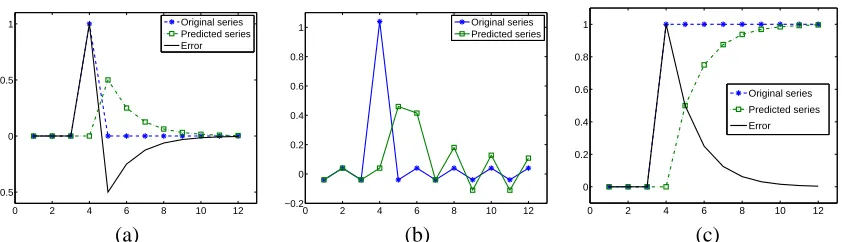
Figure 1: Holt-Winters prediction for time series with abrupt changes. (a) Impulse effect on a leveled signal: slow decaying tail; (b) Impulse effect on a periodic signal: ripple effect; (c) Response to a step signal.

of Tt and It in Eqs. (3) and (4). Based on past information, Tt and It are expected to be Tt−1and It−d under the implicit assumption of constant linear growth and fixed season. On the other hand, the current xt and the newly computed Lt suggest Tt to be Lt−Lt−1, and It to be xt−Lt. Applying

convex combination leveraging past and current information, we obtain Eqs. (3) and (4).

To start the recursion in the HW procedure at time t, initial values are needed for Lt−1, Tt−1,

and It−τ,τ=1,2, ...,d. We use the first period of data{x1,x2, ...,xd}for initialization, and start the

recursion at t=d+1. Specifically, linear regression is conducted for{x1,x2, ...,xd}versus the time

grid{1,2, ...,d}. That is, xτ andτ,τ=1, ...,d, are treated as dependent variable and independent

variable respectively. Suppose the regression function obtained is b1τ+b2. We initialize by setting L_τ=b1τ+b2, Tτ=0, and Iτ=xτ−Lτ,τ=1,2, ...,d.

The forecasting of h time units forward at t, that is, the prediction of xt+hbased on{x1,x2, ...,xt},

is

ˆ

xt+h=Lt+hTt+It−d+h mod d,

where mod is the modulo operation. The linear function of h, Lt+hTt, with slope given by the most

updated linear growth Tt, can be regarded as an estimation for Lt+h; while It−d+h mod d, the most

updated season at the same cyclic position as t+h, which is already available at t, is the estimation

for It+h.

Experiments using the HW procedure show that the local linear growth term, Tt, helps little in

prediction. In fact, for relatively distant future, the linear growth term degrades performance. This is because for the Web page view series, we rarely see any linear trends visible over a time scale from which the gradient can be estimated by HW. We can remove the term Tt in HW conveniently

by initializing it with zero and setting the corresponding smoothing parameterκ=0.

The influence of an impulse on the prediction by the HW procedure is elaborated in Figure 1. In Figure 1(a), a flat leveled series with an impulse is processed by HW. The predicted series attempts to catch up with the impulse after one lag. Although the impulse is over after one lag, the predicted series attenuates slowly, causing large errors several lags later. The stronger the impulse is, the slower the predicted series returns close to the original one. The prediction error consumes a positive value and then a negative one, both of large magnitudes. Apparently, a negative impulse will result in a reversed error pattern. Figure 1(b) shows the response of HW to an impulse added to a periodic series. The prediction error still yields the pattern of switching signs and large magnitudes. To reduce the influence of an impulse, it is important that we differentiate an impulse from a sudden step-wise change in the series. When a significant step appears, we want the predicted series to catch up with the change as fast as possible rather than hindering the strong response. Figure 1(c) shows the prediction by HW for a series with a sudden positive step change. The prediction error takes a large positive value and reduces gradually to zero without crossing into the negative side.

Based on the above observations, we detect an impulse by examining the co-existence of errors with large magnitudes and opposite signs within a short window of time. In our experiments, the window size is s1=10. The extremity of the prediction error is measured relatively with respect

to the standard deviation of prediction errors in the most recent past of a pre-selected length. In the current experiment, this length is s2=50. The time units of s1 and s2 are the same as that

of the time series in consideration. Currently, we manually set the values of s1,2. The rationale for

choosing these values is that s1implies the maximum length of an impulse; and s2balances accurate

estimation of the noise variance and swift adaptation to the change of the variance over time. We avoid setting s1too high to ensure that a detected impulse is a short-lived, strong, and abrupt change.

If a time series undergoes a real sudden rising or falling trend, the prediction algorithm will capture the trend but with a certain amount of delay, as shown by the response of HW to a step signal in Figure 1(c). In a special scenario when an impulse locates right at the boundary of a large rising trend, the measure taken to treat the impulse will further slow down the response to, but not prevent the eventual catch-up of the rise.

At time t, let the prediction for xt based on the past series up to t−1 be ˆxt, and the prediction

error be et =xt−xtˆ. We check whether an impulse has started at t0, t−s1+1≤t0≤t−1, and ended

at t by the following steps.

1. Compute the standard deviation with removed outliers, σt−1, for the prediction errors

{et−s2,et−s2+1, ...,et−1}, which are known by time t. The motivation for removing the outliers

is that at any time an impulse exists, the prediction error will be unusually large, and hence bias the estimated average amount of variation. In our experiments, 10% of the errors are removed as outliers.

2. Compute the relative magnitude of et byθt =_σt|e₋t|₁.

3. Examineθt0 in the window t0∈[t−s₁+1,t]. If there is a t0, t−s₁+1≤t0≤t−1, such that

θt0 >∆₁andθ_t>∆₂and sign(et0)6=sign(et), the segment[t0,t]is marked as an impulse. If e_t0 is positive while et negative, the impulse is a surge; the reverse is a dip. The two thresholds

∆1and∆2determine the sensitivity to impulses and are chosen around 2.5.

If impulse is not detected, the HW recursion is applied at the next time unit t+1. Otherwise, Lt, Tt,

and It0 for t0∈[t−s1+1,t], are revised as follows to reduce the effect of the impulse on the future

L_t T_t I_t

Update , ,

I_t I_t−1 I_t−s1+1

L_t

Adjust , , ...,

and

Forecast future at t

t+1 −−> t Does impulse exist?

Yes

No

Estimate parameters H and Q based on series up to time t, using Kalman filtering and the EM algorithm

Initialize Kalman filter at τ=1

τ=t?

t+1−−> t No

τ+1−−> τ

Yes

Update Kalman filter at τ

based on that at τ−1

Kalman filtering result Forecast future at t based on Detect impulse and adjust the series up to t, using the HW procedure

2D+1−−> t

L_t I_t

Apply HW recursion to

obtain and

Forecast at time t

a new year? Does t enter

Lτ

Apply ESSF to in the immediate

past two years to obtain yearly season

Iτ τ=1,2,..., 2D

Lτ Apply HW to obtain level

and weekly season at

Compute global linear trend using level subtracted by yearly season

Yes

No t+1−−> t

(a) (b) (c)

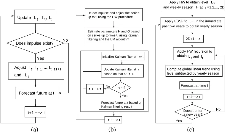
Figure 2: The schematic diagrams for the forecasting algorithms: (a) Holt-Winters with impulse detection; (b) GLS; (c) ESSF.

1. For t0=t−s1+1, ...,t, set It0 =I_t0_−d sequentially. This is equivalent to discarding the sea-son computed during the impulse segment and using the most recent seasea-son right before the impulse.

2. Let Lt =1₂Lt−s1+1₂(xt−It), where Lt−s1 is the level before the impulse and It is the already

revised season at t.

3. Let Tt =0.

In this paper, we constrain our interest to reducing the adverse effect of an impulse on later predic-tion after it has occurred and been detected. Predicting the arrival of impulses in advance using side information, for instance, scheduled events impacting Web visits, is expected to be beneficial, but is beyond our study here. A schematic diagram of the HW procedure is illustrated in Figure 2(a).

Holt-Winters and our impulse-resistant modification have the merit of being very cheap to up-date and predict, requiring only a handful of additions and multiples. This may be useful in some extremely high throughput situations, such as network routers. But in more conventional settings, it leads to the question: can we do better with more extensive model estimation at each time step?

3. State Space Model

with Gaussian noise. In general, an SSM can be represented in the following matrix form:

xt = Ztαt+εt, εt ∼N(0,Ht), (6)

αt+1 = Ttαt+Rtηt, ηt∼N(0,Qt), t=1, ...,n,

α1∼N(a1,P1)

where{α1,α2, ...,αn}is the state process. Each state is an m-dimensional column vector. Although

in our work, the observed series xt is univariate, SSM treats generally p-dimensional series. The

noise termsεt andηt follow Gaussian distributions with zero mean and covariance matrices Ht and

Qt respectively. For clarity, we list the dimension of the matrices and vectors in (6) below.

observation xt p×1 Zt p×m

state αt m×1 Tt m×m

noise εt p×1 Ht p×p

noise ηt r×1 Rt m×r

Qt r×r

initial state mean a1 m×1 P1 m×m

We restrict our interest to time invariant SSM where the subscript t can be dropped for Z, T, R, H, and Q. Matrices Z, T and R characterize the intrinsic relationship between the state and the observed series, as well as the transition between states. They are determined once we decide upon a model. The covariance matrices H and Q are estimated based on the time series using the Maximum Likelihood (ML) criterion.

Next, we describe the Level with Season (LS) model, which decomposes xt in the same way as

the HW procedure in Eq. (2)∼(4), with the linear growth term removed. We discard the growth term because, as mentioned previously, this term does not contribute in the HW procedure under our experiments. However, if necessary, it would be easy to modify the SSM to include this term. We then describe the Generalized Level with Season (GLS) model that can explicitly control the smoothness of the level.

3.1 The Level with Season Model

Denote the level at t by µt and the season with period d by it. The LS model assumes

xt = µt+it+εt,

it = −

d−1

∑

it−j+η1,t, (7)

µt = µt−1+η2,t

whereεt andηj,t, j=1,2, are the Gaussian noises.

Comparing with the HW recursion equations (2)∼(4), Eq. (7) is merely a model specifying the statistical dependence of xt on µt and it, both of which are unobservable random processes.

The Kalman filter for this model, playing a similar role as Eqs. (2)-(4) for HW, will be computed recursively to estimate µt, it, and to predict future. Details on the Kalman filter are provided in

filter for the LS model without season. The smoothing parameterζis determined by the parameters of the noise distributions in LS. When season is added, there is no complete match between the recursion of HW and that of the Kalman filter. In the LS model, it is assumed that ∑d_τ=1it+τ=0

up to white noise, but HW does not enforce the zero sum of one period of the season terms. The decomposition of xt into level µt and season it by LS is however similar to that assumed by HW.

We can cast the LS model into a time invariant SSM following the notation of (6). The matrix expansion according to (6) leads to the same set of equations in (7):

αt =

       it it−1 .. .

it−d+2 µt       

, ηt =

η

1,t

η2,t

,

Z= (1,0,0,· · ·,0,1) d×1 ,

R=          1 0 0 0 0 0 .. . ... 0 0 0 1         

d×3

, T=         

−1 −1 −1 · · · −1 0

1 0 0 · · · 0 0

0 1 0 · · · 0 0

..

. ... . .. ... ... ...

0 0 · · · 1 0 0

0 0 · · · 0 0 1

        

d×d

.

3.2 Generalized Level with Season Model

We generalize the above LS model by imposing different extent of smoothness on the level term µt.

Specifically, let

xt = µt+it+εt, (8)

it = −

s−1

∑

it−j+η1,t,

µt = 1 q

q

∑

µt−j+η2,t .

Here q≥1 controls the extent of smoothness. The higher the q, the smoother the level{µ1,µ2, ...,µn}.

We experiment with q=1,3,7,14.

Again, we cast the model into an SSM. The dimension of the state vector is m=d−1+q.

αt =

          it .. .

it−d+2 µt

.. .

µt−q+1

         

, ηt=

η1,t

η2,t

We describe Z, R, T by the sparse matrix format. Denote the (i,j)th element of a matrix, for example, T, by T(i,j)(one index for vectors). An element is zero unless specified.

Z= [Z(i,j)]1×m, Z(1) =1,Z(d) =1,

R= [R(i,j)]m×2, R(1,1) =1,R(d,2) =1,

T= [T(i,j)]m×m, T(1,j) =−1, j=1,2, ...,d−1,

T(1+j,j) =1, j=1,2, ...,d−2,

T(d,d−1+j) =1

q, j=1, ...,q,

T(d+j,d−1+j) =1,j=1,2, ...,q−1,if q>1.

We compare the LS and GLS models in Section 5 by experiments. It is shown that for distant prediction, imposing smoothness on the level can improve performance.

In practice, the prediction of a future xt+hbased on{x1,x2, ...,xt}comprises two steps:

1. Estimate H and Q in GLS (or SSM in general) using the past series{x1, ...,xt}.

2. Estimate xt+hby the conditional expectation E(xt+h|x1,x2, ...,xt)under the estimated model.

We may not need to re-estimate the model with every new coming xt, but update the model once

every batch of data. We estimate the model by the ML criterion using the EM algorithm. The Kalman filter and smoother, which involve forward and backward recursion respectively, are the core of the EM algorithm for SSM. Given an estimated model, the Kalman filter is used again to compute E(xt+h|x1,x2, ...,xt), as well as the variance Var(xt+h|x1,x2, ...,xt): a useful indication for

the prediction accuracy. Details on the algorithms for estimating SSM and making prediction based on SSM are provided in the Appendix. A thorough coverage on the theories of SSM and related computational methods is referred to Durbin and Koopman (2001).

Because treating impulses improves prediction, as demonstrated by the experiments in Sec-tion 5, it is conducted for the GLS approach. In particular, we invoke the impulse detecSec-tion embed-ded in HW. For any segment of time where an impulse is marked, the observed data xt are replaced

by Lt+It computed by HW. This modified series is then input to the GLS estimation and prediction

algorithms. The schematic diagram for forecasting using GLS is shown in Figure 2(b).

4. Long-range Trend and Seasonality

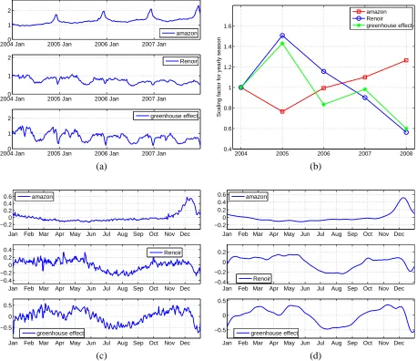
Web page views sometimes show long-range trend and seasonality. In Figure 7(a), three time series over a period of four years are shown. Detailed description of the series is provided in Section 5. Each time series demonstrates apparently a global trend and yearly seasonality. For instance, the first series, namelyamazon, grows in general over the years and peaks sharply every year around December. Such long-range patterns can be exploited for forecasting, especially for distant future. To effectively extract long-range trend and season, several needs ought to be addressed:

2. A mechanism to control the smoothness of the long-range season is needed. By enforcing smoothness, the extracted season tends to be more robust, a valuable feature especially when given limited past data.

3. The magnitude of the yearly season may vary across the years. As shown in Figure 7(a), although the series over different years show similar patterns, the patterns may be amplified or shrunk over time. The yearly season thus should be allowed to scale.

The HW and GLS approaches fall short of meeting the above requirements. They exploit mainly the local statistical dependence in the time series. Because HW (and similarly GLS) performs essentially exponential smoothing on the level and linear growth terms, the effect of historic data further away attenuates fast. HW is not designed to extract a global trend over multiple years. Furthermore, HW requires a relatively large number of periods to settle to the intended season; and importantly, HW assumes a fixed season over the years. Although HW is capable of adjusting with a slowly changing season when given enough periods of data, it does not directly treat the scaling of the season, and hence is vulnerable to the scaling phenomenon.

In our study, we adopt a linear regression approach to extract the long-range trend. We inject elasticity into the yearly season and allow it to scale from a certain yearly pattern. The algorithm developed is called Elastic Smooth Season Fitting (ESSF). The time unit of the series is supposed to be a day.

4.1 Elastic Smooth Season Fitting

Before extracting long-range trend and season, we apply HW with impulse detection to obtain the weekly season and the smoothed level series Lt, t=1, ...,n. Recall that the HW prediction for

the level Lt+h at time t is Lt, assuming no linear growth term in our experiments. We want to

exploit the global trend and yearly season existing in the level series to better predict Lt+hbased on

{L1,L2, ...,Lt}.

We decompose the level series Lt, t=1, ...,n, into a yearly season, yt, a global linear trend ut,

and a volatility part nt:

Lt=ut+yt+nt , t=1,2, ...,n.

Thus the original series xt is decomposed into:

xt =ut+yt+nt+It+Nt, (9)

where Itand Ntare the season and noise terms from HW. Let u={u1,u2, ...,un}and y={y1,y2, ...,yn}.

They are solved by the following iterative procedure. At this moment, we assume the ESSF algo-rithm, to be described shortly, is available. We start by setting y(0)=0. At iteration p, update y(p) and u(p)by

1. Let gt =Lt−y(tp−1), t=1, ...,n. Note gt is the global trend combined with noise, taking out

the current additive estimate of the yearly season.

2. Perform linear regression of g={g1, ...,gn}on the time grid {1,2, ...,n}. Let the regressed value at t be u(tp), t=1,2, ...,n. Thus for some scalars b(

p) 1 and b

(p) 2 , u

(p) t =b(

p) 1 t+b

3. Let zt =Lt−ut(p), t=1, ...,n. Here zt is the yearly season combined with noise, taking out the

current estimate of the global trend. Apply ESSF to z={z1,z2, ...,zn}. Let the yearly season

derived by ESSF be y(p)_.

It is analytically difficult to prove the convergence of the above procedure. Experiments based on three series show that the difference in y(p)reduces very fast. At iteration p, p≥2, we measure the relative change from y(p−1)to y(p)by

||y(p)−y(p−1)||

||y(p−1)|| , (10)

where|| · ||is the L2norm. Detailed results are provided in Section 5. Because ESSF always has to

be coupled with global trend extraction, for brevity, we also refer to the entire procedure above as ESSF when the context is clear, particularly, in Section 4.2 and Section 5.

We now present the ESSF algorithm for computing the yearly season based on the trend removed z. For notational brevity, we re-index day t by double indices(k,j), which indicates day t is the jth day in the kth year. Denote the residue zt =Lt−ut by zk,j, the yearly season yt by yk,j (we abuse

the notation here and assume the meaning is clear from the context), and the noise term nt by nk,j.

Suppose there are a total of K years and each contains D days. Because leap years contain one more day, we take out the extra day from the series before applying the algorithm.

We call the yearly season pattern y={y₁,y₂, ...,y_D} the season template. Since we allow the yearly season yk,jto scale over time, it relates to the season template by

yk,j=αk,jyj, k=1,2, ...,K, j=1, ...,D,

whereαk,j is the scaling factor. One choice forαk,j is to letαk,j =ck, that is, a constant within

any given year. We call this scheme step-wise constant scaling sinceαk,j is a step function if single

indexed by time t. One issue with the step-wise constant scaling factor is that yk,j inevitably jumps

when entering a new year. To alleviate the problem, we instead use a piece-wise linear function for αk,j. Let c0=1. Then

αk,j= j−1

D ck+

D−j+1

D ck−1, k=1,2, ...,K, j=1, ...,D. (11)

The number of scaling factors ckto be determined is still K. Let c={c1, ...,cK}. At the first day of

each year,αk,1=ck−1. We optimize over both the season template yj, j=1, ...,D, and the scaling

factors ck, k=1, ...,K.

We now have

zk,j=αk,jyj+nk,j,

where zk,j’s are given, while ck, yj, and nk,j, k=1, ...,K, j=1, ...,D, are to be solved. A natural

optimization criterion is to minimize the sum of squared residues:

min

y,c

∑

∑

2

k,j=min

y,c

∑

∑

2_.

If the number of years K is small, y obtained by the above optimization can be too wiggly. We add a penalty term to ensure the smoothness of y. The discrete version of the second order derivative for y_j is

and∑j¨y 2

j is used as the smoothness penalty. Since y is one period of the yearly season, when j0is

out of the range[1,D], y_j0 is understood as y_j0_{mod D}. For instance, y₀=y_D, y_D+1=y₁. We form the following optimization criterion with a pre-selected regularization parameterλ:

min

y,c G(y,c) =miny,c

∑

∑

2_+λ

∑

(y_j+1+y_j−1−2y_j)2. (12)

To solve(12), we alternate the optimization of y and c. With either fixed, G(y,c)is a convex quadratic function. Hence a unique minimum exists and can be solved by a multivariable linear equation. The algorithm is presented in details in Appendix B.

Experiments show that allowing scalable yearly season improves prediction accuracy, so does the smoothness regularization of the yearly season. As long asλis not too small, the prediction performance varies marginally for a wide range of values. The sensitivity of prediction accuracy to λis studied in Section 5.

A more ad-hoc approach to enforce smoothness is to apply moving average to the yearly season extracted without smoothness regularization. We can further simplify the optimization criterion in (12) by employing step-wise constant scaling factor, that is, letαk,j =ck, k=1, ...,K. The jump

effect caused by the abrupt change of the scaling factor is reduced by the moving average as well. Specifically, the optimization criterion becomes

min

y,c

˜

G(y,c) =min

y,c

∑

∑

2_{. (13)}

The above minimization is solved again by alternating the optimization of y and c. See Appendix B for details. Comparing with Eq. (12), the optimization for (13) reduces computation significantly. After acquiring y, we apply a double sided moving average. We call the optimization algorithm for (13) combined with the post operation of moving average the fast version of ESSF. Experiments in Section 5 show that ESSF Fast performs similarly to ESSF.

4.2 Prediction

We note again that ESSF is for better prediction of the level Lt obtained by HW. To predict xt, the

weekly season extracted by HW should be added to the level Lt. The complete process of prediction

is summarized below. We assume that prediction starts on the 3rd year since the first two years have to serve as past data for computing the yearly season.

1. Apply HW to obtain the weekly season It, and the level Lt, t=1,2, ...,n.

2. At the beginning of each year k, k=3,4, ..., take the series of Lt’s in the past two years (year k−2 and k−1) and apply ESSF to this series to solve the yearly season template y and the scaling factors, c1 and c2 for year k−2 and k−1 respectively. Predict the yearly season for

future years k0≥k by c2y. Denote the predicted yearly season at time t in any year k0≥k by Yt,k, where the second subscript clarifies that only the series before year k is used by ESSF.

3. Denote the year in which day t lies byν(t). Let the yearly season removed level be ˜Lt=Lt− Yt,ν(t). At every t, apply linear regression to{˜Lt−2D+1, ...,˜Lt}over the time grid{1,2, ...,2D}.

2006 Nov 2006 Dec 2007 Jan 0

0.1 0.2 0.3 0.4 0.5

Weekly season Yearly season Long−range growth

2006 Nov 2006 Dec 2007 Jan 1.4

1.6 1.8 2 2.2 2.4

Original series ESSF HW Level

(a) (b)

Figure 3: Decomposition of the prediction terms for theamazonseries in November and December of 2006 based on data up to October 31, 2006: (a) The weekly season, yearly season, and long-range linear growth terms in the prediction; (b) Comparison of the predicted series by HW and ESSF.

Suppose at the end of day t (or beginning of day t+1), we predict for the hth day ahead of t. Let the prediction be ˆxt+h. Also let r(t+h)be the smallest integer such that t+h−r(t+h)·d≤t

(d is the weekly period). Then,

ˆ

xt+h= ˜Lt+h ˜Tt+Yt+h,ν(t)+It+h−r(t+h)·d. (14)

Drawing a comparison between Eqs. (14) and (9), we see that ˜Lt+h ˜Tt is essentially the

predic-tion for the global linear trend term ut+h, Yt+h,ν(t) the prediction for the yearly season yt+h, and It+h−r(t+h)·d the prediction for the weekly season It+h. The schematic diagram for forecasting by

ESSF is shown in Figure 2(c).

If day t+h is in the same year as t, Yt+h,ν(t)=Yt+h,ν(t+h)is the freshest possible prediction for the

yearly season at t+h. If insteadν(t)<ν(t+h), the yearly season at t+h is predicted based on data

more than one year ago. One might have noticed that we use only two years of data to extract the yearly season regardless of the available amount of past data. This is purely an individual choice due to our preference of using recent data. Experiments based on the series described in Section 5 show that whether all the available past data are used by ESSF causes negligible difference in prediction performance.

5. Experiments

We conduct experiments using twenty six time series. As a study of the characteristics of Web page views, we examine the significance of the seasonal as well as impulsive variations. Three relatively short series are used to assess the performance of short-term prediction by the HW and GLS approaches. The other twenty three series are used to test the ESSF algorithm for long-term prediction. In addition to comparing the different forecasting methods, we also present results to validate the algorithmic choices made in ESSF.

5.1 Data Sets

We conduct experiments based on the time series described below.

1. TheAutonseries records the daily page views of the Auton Lab, headed by Andrew Moore, in the Robotics Institute at the Carnegie Mellon University (http://www.autonlab.org). This series spans from August 14, 2005 to May 1, 2007, a total of 626 days.

2. TheWangseries records the daily page views of the Web site for the research group headed by James Wang at the Pennsylvania State University (http://wang.ist.psu.edu). This series spans from January 1, 2006 to February 1, 2008, a total of 762 days.

3. Theciteseerseries records the hourly page views to citeseer, an academic literature search engine currently located at http://citeseer.ist.psu.edu. This series spans from 19 : 00 on Septem-ber 6, 2005 to 4 : 00 on SeptemSeptem-ber 25, 2005, a total of 442 hours.

4. We acquired 23 relatively long time series from the site http://www.google.com/trends. This Web site provides search volumes for user specified phrases. We treat the search volumes as an indication of the page views to dynamically generated Web pages by Google. The series record daily volumes from Jan, 2004 to December 30, 2007 (roughly four full years), a total of 1460 days. The volumes for each phrase are normalized with respect to the average daily volume of that phrase in the month of January 2004. The normalization will not affect the prediction accuracy, which is measured relatively with respect to the average level of the series. We also call the series collectively theg-trendsseries.

5.2 Evaluation

Let the prediction for xt be ˆxt. Suppose prediction is provided for a segment of the series,

{xt0+1,xt0+2, ...,xt0+J}, where 0≤t0<n. We measure the prediction accuracy by the error rate

defined as

Re=

r

RSS SSS

where RSS, the residual sum of squares is

RSS= t0+J

∑

(xˆt−xt)2 (15)

and SSS, the series sum of squares is

SSS= t0+J

∑

We call Rethe prediction error rate. It is the reciprocal of the square root of the signal to noise ratio

(SNR), a measure commonly used in signal processing. We can also evaluate the effectiveness of a prediction method by comparing RSS to SPV , the sum of predictive variation:

SPV = t0+J

∑

(xt−xt)2, xt=∑ t−1

τ=1xτ t−1 .

We can consider xt, the mean up to time t−1, as the simplest prediction of xtusing past data. We call

this scheme of prediction Mean of Past (MP). SPV is essentially the RSS corresponding to the MP method. The Re of MP is

p

SPV/SSS. We denote the ratio between the Reof a prediction method and that of MP by Qe=

p

RSS/SPV , referred to as the error ratio. As a measure on the amount of

error, in practice, Reis more pertinent than Qefor users concerned with employing the prediction in

subsequent tasks. We thus use Reas the major performance measure in all the experimental results.

For comparison with baseline prediction methods, we also show Re of MP as well as that of the

Moving Average (MA). In the MA approach, considering the weekly seasonality, we treat Monday to Sunday separately. Specifically, if a day to be predicted is a Monday, we forecast by the average of the series on the past 4 Mondays. Similarly for the other days of a week. For the hourly page view series with daily seasonality, MA predicts by the mean of the same hours in the past 4 days.

As discussed previously, Web page views exhibit impulsive changes. The prediction error during an impulse is extraordinarily large, skewing the average error rate significantly even if impulses only exist on a small fraction of the series. The bias caused by the outlier errors is especially strong when the usual amount of page views is low. We reduce the effect of outliers by removing a small percentage of large errors, in particular, 5% in our experiments. Without loss of generality, suppose the largest (in magnitude) 5% errors are ˆxt−xt at t0+1≤t≤t1. We adjust RSS and SSS by using

only ˆxt−xt at t>t1and compute the corresponding Re. Specifically,

RSSad j= t0+J

∑

(xˆt−xt)2,SSSad j= t0+J

∑

x2_t ,Rad j_e =

s

RSSad j SSSad j .

We report both Reand Rad je to measure the prediction accuracy for the seriesAuton,Wang, and

citeseer. For the twenty threeg-trendsseries, because there is no clear impulse, we use only

Re.

Because the beginning portion of the series with a certain length is needed for initialization in HW, SSM, or ESSF, we usually start prediction after observing t0>0 time units. Moreover, we may

predict several time units ahead for the sum of the series over a run of multiple units. The ground truth at t is not necessarily xt. In general, suppose prediction starts after t0and is always for a stretch

of w time units that starts h time units ahead. We call w the window size of prediction and h the unit

ahead.

Let the whole series be{x1,x2, ...,xn}. In the special case when h=1 and w=1, after observing

the series up to t−1, we predict for xt, t=t0+1, ...,n. The ground truth at t is xt. If h≥1, w=1,

we predict for xt, t=t0+h, ...,n, after observing the series up to t−h. Let the predicted value be

ˆ

xt,−h, where the subscript−h emphasizes that only data h time units ago are used. If h≥1, w≥1,

we predict for

˜

xt= t+w−1

∑

τ=t

after observing the series up to t−h. The predicted value at t is

ˆ˜xt= t+w−1

∑

τ=t

ˆ

xτ,−h.

To compute the error rate Re, we adjust RSS and SSS in Eq. (15) and (16) according to the ground

truth:

RSS= n−w+1

∑

(ˆ˜xt−x˜t)2, SSS= n−w+1

∑

˜

x2_t .

For the seriesAuton,Wang, andciteseer, t0=4d, where d is the season period. The segment

{x1, ...,x4d}is used for initialization by both HW and SSM. For theg-trendsseries, t0=731. That

is, the first two years of data are used for initialization. Two years of past data are needed because the ESSF algorithm requires at least two years of data to operate.

5.3 Results

For the seriesAuton,Wang, andciteseer, we focus on short-term prediction no greater than 30 time units ahead. Because the series are not long enough for extracting long-range trend and season by the ESSF algorithm, we only test the HW procedure with or without impulse detection and the GLS approach. For the twenty threeg-trendsseries, we compare ESSF with HW for prediction up to half a year ahead.

5.3.1 SHORT-TERMPREDICTION

Web page views often demonstrate seasonal variation, sometimes at multiple scales. The HW pro-cedure given by Eq. (2)∼(4) and the GLS model specified in Eq. (8) both assume a season term with period d. In our experiments, for the daily page view seriesAutonandWang, d=7 (a week), while for the hourly series citeseer, d=24 (a day). As mentioned previously, the local linear growth term in Eq. (3) is removed in our experiments because it is found not helpful. The smooth-ing parameters for the level and the season terms in Eq. (2) and (4) are set toζ=0.5 andδ=0.25. Because HW has no embedded mechanism to select these parameters, we do not aggressively tune them and use the same values for all the experiments reported here.

To assess the importance of weekly (or daily) seasonality for forecasting, we compare HW and and its reduced form without the season term. Similarly as the linear growth term, the season term can be deleted by initializing it to zero and setting its corresponding smoothing parameterδ in Eq. (4) to zero. The reduced HW procedure without the local linear growth and season terms is essentially Exponential Smoothing (ES) (Chatfield, 2004). Figure 4(a) compares the prediction performance in terms of Reand Rad je for the three series by HW and ES. Results for two versions of

HW, with and without treating impulses, are provided. The comparison of the two versions will be discussed shortly. Results obtained from the two baseline methods MA and MP are also shown. For each of the three series, HW (both versions), which models seasonality, consistently outperforms ES, reflecting the significance of seasonality in these series. We also note that for theautonseries,

Re is almost twice as large as Rad je although only 5% of outliers are removed. This dramatic skew

of the error rate is caused by the short but strong impulses occurred in this series.

Auton Wang citeseer 0 10 20 30 40 50 60

Error rate (%)

HW (Imp.), R_eadj

HW (No imp.), R_eadj

ES, R e adj

HW (Imp.), R e HW (No imp.), R

e ES, R e MA, R e MP, R e 1 −6 −4 −2 0 2 4 6

x 104

Value Auton 1 −1.5 −1 −0.5 0 0.5 1 1.5

x 104

Wang 1 −1.5 −1 −0.5 0 0.5 1 1.5

x 104

Citeseer

(a) (b)

Figure 4: Compare the prediction performance in terms of Rad je and Reon the three seriesAuton,

Wang, andciteseerusing different methods: HW with or without impulse detection, ES without season, MA, and MP. (a) The error rates. (b) The box plots for the differences of page views at adjacent time units.

The decrease in error rate for the other two series is small, a result of the fact there is no strong impulse in them. To directly demonstrate the magnitude of the impulses, we compute the differences in page view between adjacent time units,{x2−x1,x3−x2, ...,xn−xn−1}, and show the box plots for their distributions in Figure 4(b). The stronger impulses inAutonare evident from the box plots. Comparing with the other two series, the middle half of theAutondata (between the first and third quartiles), indicated by the box in the plot, is much narrower relative to the overall range of the data. In another word, the outliers deviate more severely from the majority mass of the data.

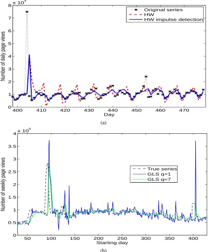
To illustrate the gain from treating impulses, we also show the predicted series for Auton in Figure 5(a). For clarity of the plot, only a segment of the series around an impulse is shown. The predicted series by HW with impulse detection returns close to the original series shortly after the impulse, while that without ripples with large errors over several periods afterward. In the sequel, for both HW and GLS, impulse detection is included by default.

Table 1 lists the error rates for the three series using different methods and under different pairs of(h,w), where h is the unit ahead and w is the window size of prediction. We provide the error rate

Rad je in addition to Reto show the performance on impulse excluded portion of the series. ForAuton

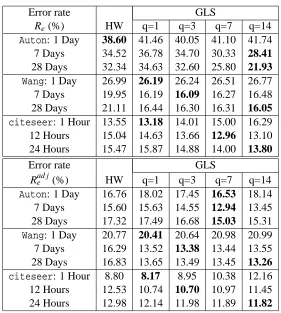
andWang,(h,w) = (1,1),(1,7),(1,28). Forciteseer,(h,w) = (1,1),(1,12),(1,24). For the GLS model, a range of values for the smooth parameter q are tested. As shown by the table, when

(h,w) = (1,1), the performance of HW and that of GLS at the best q are close. When predicting multiple time units, for example, w=7,28 or w=12,24, GLS with q>1 achieves better accuracy. For Wang andciteseer, at every increased w, the lowest error rates are obtained by GLS with an increased q. This supports the heuristic that when predicting for a more distant time, smoother prediction is preferred to reduce the influence of local fluctuations.

400 410 420 430 440 450 460 470 0

1 2 3 4 5 6 7

8x 10

4

Day

Number of daily page views

Original series HW

HW impulse detection

(a)

50 100 150 200 250 300 350 400

0 0.5 1 1.5 2 2.5 3 3.5

4x 10

5

Starting day

Number of weekly page views

True series GLS q=1 GLS q=7

(b)

Error rate GLS

Re(%) HW q=1 q=3 q=7 q=14

Auton: 1 Day 38.60 41.46 40.05 41.10 41.74 7 Days 34.52 36.78 34.70 30.33 28.41 28 Days 32.34 34.63 32.60 25.80 21.93 Wang: 1 Day 26.99 26.19 26.24 26.51 26.77 7 Days 19.95 16.19 16.09 16.27 16.48 28 Days 21.11 16.44 16.30 16.31 16.05 citeseer: 1 Hour 13.55 13.18 14.01 15.00 16.29 12 Hours 15.04 14.63 13.66 12.96 13.10 24 Hours 15.47 15.87 14.88 14.00 13.80

Error rate GLS

Rad je (%) HW q=1 q=3 q=7 q=14

Auton: 1 Day 16.76 18.02 17.45 16.53 18.14 7 Days 15.60 15.63 14.55 12.94 13.45 28 Days 17.32 17.49 16.68 15.03 15.31 Wang: 1 Day 20.77 20.41 20.64 20.98 20.99 7 Days 16.29 13.52 13.38 13.44 13.55 28 Days 16.83 13.65 13.49 13.45 13.26 citeseer: 1 Hour 8.80 8.17 8.95 10.38 12.16 12 Hours 12.53 10.74 10.70 10.97 11.45 24 Hours 12.98 12.14 11.98 11.89 11.82

Table 1: The prediction error rates Re and Rad je for the three series Auton, Wang, and citeseer

obtained by several methods. The window size of prediction takes multiple values, while the unit ahead is always 1. HW and the GLS model with several values of q are compared.

by q=1 is more volatile than that by q=7. The volatility of the predicted series by q=7 is much closer to that of the true series. As shown in Table 1, the error rate Rad je achieved by q=7 is 12.94%,

while that by q=1 is 15.63%.

Based on the GLS model, the variance of xt conditioned on the past{x1, ...,xt−1}can be

com-puted. The equations for the conditional mean E(xt |x1, ...,xt−1) (i.e., the predicted value) and variance Var(xt |x1, ...,xt−1)are given in (19). Since the conditional distribution of xt is Gaussian,

we can thus calculate a confidence band for the predicted series, which may be desired in certain applications to assess the potential deviation of the true values. Figure 6 shows the 95% confidence band forciteseerwith(h,w) = (1,1). The confidence band covers nearly the entire original series. GLS is more costly in computation than HW. We conduct the experiments using Matlab codes on 2.4GHz Dell computer with Linux OS. At(h,w) = (1,28)forAutonandWang, and(h,w) = (1,24)

100 150 200 250 300 350 400 450 0.5

1 1.5 2 2.5 3 3.5 4 4.5

5x 10

4

Hour

Number of hourly page views

Original series Upper 95% CB Lower 95% CB

Figure 6: The predicted 95% confidence band forciteseerobtained by GLS with q=1. The unit ahead h and window size w are 1.

5.3.2 LONG-TERMPREDICTION—A COMPREHENSIVESTUDY

We now examine the performance of ESSF based on the g-trendsseries. The first three series are acquired by the search phrasesamazon,Renoir(French impressionism artist), andgreenhouse effect, which will be used as the names for the series in the sequel. A comprehensive study with detailed results is first presented using these three series. Then, we expand the experiments to twenty additionalg-trendsseries and present results on prediction accuracy and computational speed.

The original series ofamazon,Renoir, andgreenhouse effectaveraged weekly are shown in Figure 7(a). Due to the weekly season, without averaging, the original series are too wiggly for clear presentation. Figure 7(c) and (d) show the yearly season templates extracted by ESSF from year 2004 and 2005 with smoothing parameterλ=0, 1000 respectively. As expected, atλ=1000, the yearly seasons are much smoother than those obtained atλ=0, especially for the seriesRenoir andgreenhouse effect. Figure 7(b) shows the scaling factors of the yearly seasons obtained by applying ESSF to the entire four years.

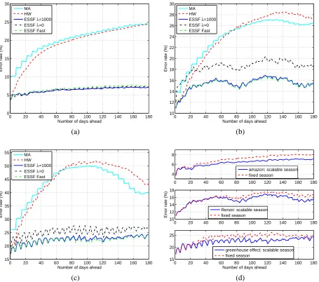
We compare the prediction obtained by ESSF with HW and the MA approach as a baseline. For ESSF, we test bothλ=0 and 1000, and its fast version with moving average window size 15. Prediction error rates are computed for the unit ahead h ranging from 1 to 180 days. We fix the prediction window size w=1.

The error rates Re obtained by the methods are compared in Figure 8(a), (b), (c) foramazon,

2004 Jan0 2005 Jan 2006 Jan 2007 Jan 1

2

2004 Jan0 2005 Jan 2006 Jan 2007 Jan 1

2

2004 Jan0 2005 Jan 2006 Jan 2007 Jan 1

2

amazon

Renoir

greenhouse effect

2004 2005 2006 2007 2008 0.4

0.6 0.8 1 1.2 1.4 1.6

Scaling factor for yearly season

amazon Renoir greenhouse effect

(a) (b)

Jan Feb Mar Apr May Jun Jul Aug Sep Oct Nov Dec −0.2

0 0.2 0.4 0.6

Jan Feb Mar Apr May Jun Jul Aug Sep Oct Nov Dec −0.4

−0.2 0 0.2 0.4

Jan Feb Mar Apr May Jun Jul Aug Sep Oct Nov Dec −0.5

0 0.5

amazon

Renoir

greenhouse effect

Jan Feb Mar Apr May Jun Jul Aug Sep Oct Nov Dec −0.2

0 0.2 0.4 0.6

Jan Feb Mar Apr May Jun Jul Aug Sep Oct Nov Dec −0.4

−0.2 0 0.2

Jan Feb Mar Apr May Jun Jul Aug Sep Oct Nov Dec −0.5

0 0.5

amazon

Renoir

greenhouse effect

(c) (d)

0 20 40 60 80 100 120 140 160 180 0 5 10 15 20 25 30

Number of days ahead

Error rate (%)

MA HW ESSF λ=1000 ESSF λ=0 ESSF Fast

0 20 40 60 80 100 120 140 160 180 10 12 14 16 18 20 22 24 26 28 30

Number of days ahead

Error rate (%)

MA HW ESSF λ=1000 ESSF λ=0 ESSF Fast

(a) (b)

0 20 40 60 80 100 120 140 160 180 15 20 25 30 35 40 45 50 55

Number of days ahead

Error rate (%)

MA HW ESSF λ=1000 ESSF λ=0 ESSF Fast

0 20 40 60 80 100 120 140 160 180 4

6 8

0 20 40 60 80 100 120 140 160 180 10

12 14 16 18

Error rate (%)

0 20 40 60 80 100 120 140 160 180 15

20 25

Number of days ahead

amazon: scalable season fixed season

Renoir: scalable season fixed season

greenhouse effect: scalable season fixed season

(c) (d)

Figure 8: Compare prediction error rates Refor threeg-trendsseries using several methods.

2 3 4 5 0

1 2 3 4 5

Iteration

Change ratio (%)

amazon Renoir

greenhouse effect

0 20 40 60 80 100 120 140 160 180 2

4 6 8 10

0 20 40 60 80 100 120 140 160 180 10

12 14 16 18

Error rate (%)

0 20 40 60 80 100 120 140 160 180 15

20 25

Number of days ahead

amazon, #ite=5 #ite=1

Renoir, #ite=5 #ite=1

greenhouse effect, #ite=5 #ite=1

(a) (b)

Figure 9: The effect of the number of iterations in the ESSF algorithm: (a) The change ratio in the extracted yearly season over the iterations; (b) Compare the error rates Re obtained by

ESSF with 1 iteration and 5 iterations respectively.

nearly the same, both achieving error rates consistently lower than those by HW. The gap between the error rates of ESSF and HW widens quickly with an increasing h. In general, when h increases, the prediction is harder, and hence the error rate tends to increase. The increase is substantially slower for ESSF than HW and MA. ESSF withλ=0 performs considerably worse thanλ=1000 for Renoirandgreenhouse effect, and closely foramazon. This demonstrates the advantage of imposing smoothness on the yearly season. We will study more thoroughly the effect of λon prediction accuracy shortly.

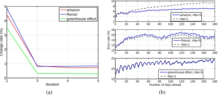
Next, we experiment with ESSF under various setups and demonstrate the advantages of several algorithmic choices. First, recall that the fitting of the yearly season and the long-range trend is repeated multiple times, as described in Section 4.1. To study the effect of the number of iterations, we plot in Figure 9(a) the ratio of change in the yearly season after each iteration, as given by Eq. (10). For all the three series, the most prominent change occurs between iteration 1 and 2 and falls below 1% for any later iterations. We also compare the prediction error rates for h=1, ...,180 achieved by using only 1 iteration (essentially no iteration) versus 5 iterations. The results for the three series are plotted in Figure 9(b). The most obvious difference is with amazon for large h. At h=180, the error rate obtained by 5 iterations is about 2% lower than by 1 iteration. On the other hand, even with only 1 iteration, the error rate at h=180 is below 10%, much lower than the nearly 25% error rate obtained by HW or MA. Forgreenhouse effect, the difference is almost imperceptible.

10−1 100 101 102 103 6.2

6.3 6.4 6.5

10−1 100 101 102 103

15 16 17 18 19

Average error rate (%)

10−1 100 101 102 103

22 24 26

λ

amazon

Renoir

greenhouse effect

Figure 10: The effect of the smoothing parameterλin ESSF on prediction accuracy. At eachλ, the average of error rates Reacross the unit ahead h=1, ...,180 are shown.

the two schemes for the three series. Better performance is achieved by allowing scalable yearly seasons for all the three series. The advantage is more substantial when predicting the distant future. To examine the sensitivity of the prediction accuracy to the smoothing parameterλ, we varyλ from 0.1 to 2000, and compute the error rates for h=1, ...,180. For concise illustration, we present the average of the error rates across h. Note that the results ofλ=0,1000 at every h are shown in Figure 8, whereλ=0 is inferior. The variation of the average error rates with respect toλ(in log scale) is shown in Figure 10. Foramazon, the error rates with differentλ’s lie in the narrow range of

[6.2%,6.45%], while forRenoirandgreenhouse effect, the range is wider, roughly[15%,18%]

and[22%,25%]respectively. For all the three series, the decrease of the error rate is most steep whenλincreases from 0.1 to 10. Forλ>10 and as large as 2000, the change in error rate is minor, indicating that the prediction performance is not sensitive toλas long as it is not too small.

5.3.3 LONG-TERMPREDICTION—EXTENDEDSTUDY ONTWENTYTRENDSERIES

We collect another twentyg-trendsseries with query phrases and corresponding series ID listed in Table 2. The error rates Re achieved by the four methods: MA, HW, ESSF withλ=1000, and

ESSF Fast, over the twenty series are compared in Figure 11. The four plots in this figure each show results for predicting a single day in advance of h days, with h=1,30,60,90 respectively. For most series, MA is inferior to HW at every h. However, when h increases, the margin of HW over MA decreases. At h=1, HW performs similarly as ESSF and ESSF Fast. At h=30,60,90, both versions of ESSF, which achieve similar error rates between themselves, outperform HW.

To assess the predictability of the series, we compute the variation rates at h=1,30,60,90, shown in Figure 12(a). The variation rate at h is defined as pVar(xt+h−xt)/

p

1 2 3 4 5 6 7 8 9 10 11 12 13 14 15 16 17 18 19 20 0 10 20 30 40 50 60 70 80

Error rate (%)

Time series ID MA HW

ESSF λ=1000

ESSF Fast

1 2 3 4 5 6 7 8 9 10 11 12 13 14 15 16 17 18 19 20 0 10 20 30 40 50 60 70 80 90 100

Error rate (%)

Time series ID MA HW ESSF λ=1000 ESSF Fast

(a) (b)

1 2 3 4 5 6 7 8 9 10 11 12 13 14 15 16 17 18 19 20 0 20 40 60 80 100 120

Error rate (%)

Time series ID MA HW ESSF λ=1000 ESSF Fast

1 2 3 4 5 6 7 8 9 10 11 12 13 14 15 16 17 18 19 20 0 20 40 60 80 100 120 140

Error rate (%)

Time series ID MA HW ESSF λ=1000 ESSF Fast

(c) (d)

Figure 11: Compare the error rates by MA, HW, ESSF withλ=1000, and ESSF Fast for twenty g-trendsseries. (a)-(d): The unit ahead h=1,30,60,90.

1 2 3 4 5 6 7 8 9 10 11 12 13 14 15 16 17 18 19 20 20 40 60 80 100 120 140 160 180

Variation rate (%)

Time series ID h=1

h=30 h=60 h=90

1 2 3 4 5 6 7 8 9 10 11 12 13 14 15 16 17 18 19 20 0.2 0.3 0.4 0.5 0.6 0.7 0.8 0.9 1

Yearly correlation coefficient

Time series ID

(a) (b)

ID Query phrase ID Query phrase 1 American idol 11 human population 2 Anthropology 12 information technology

3 Aristotle 13 martial art

4 Art history 14 Monet

5 Beethoven 15 National park

6 Confucius 16 NBA

7 Cosmology 17 photography

8 cure cancer 18 public health

9 democracy 19 Shakespeare

10 financial crisis 20 Yoga

Table 2: The query phrases for twentyg-trendsseries and their IDs.

Var(·) denotes the serial variance. This rate is the ratio between the standard deviation of the change in page view h time units apart and that of the original series. A low variation rate indicates the series is less volatile and hence likely to be easier to predict. For example,Art history(ID 4) andNational park(ID 15) have the lowest variation rates at h=1, and they both yield relatively low prediction error rates, as shown by Figure 11. We also compute the variation rates for the page views of Web sitesAuton, Wang, and citeseerat h=1. They are respectively 100.0%, 88.1%, and 48.2%. This shows that the volatility of page views at these Web sites is in a similar range as that of theg-trendsseries.

In addition to the variation rate, the yearly correlation of the time series also indicates the po-tential for accurate prediction. For each of the twentyg-trendsseries, we compute the average of the correlation coefficients between segments of the series in adjacent years (i.e., 2004/05, 05/06, 06/07). Figure 12(b) shows the results. A series with high yearly correlation tends to benefit more in prediction from the yearly season extraction of ESSF. For instance,martial art(ID 13) has relatively low yearly correlation. The four prediction methods perform nearly the same for this se-ries. In contrast, forNBA(ID 16) anddemocracy(ID 9), which have high yearly correlation, ESSF achieves substantially better prediction accuracy than HW and MA at all the values of h.

To compare the computational load of the prediction algorithms, we acquire the average user running time over the twentyg-trendsseries for one day ahead (h=1) prediction at all the days in the last two years, 2006 and 2007. Again, we use Matlab codes on 2.4GHz Dell computer with Linux OS. The average time is respectively 0.11, 0.32, 0.59, and 3.77 seconds for MA, HW, ESSF Fast, and ESSF withλ=1000.

6. Discussion and Conclusions