Efficient Learning of Label Ranking by Soft Projections onto Polyhedra

Efficient Learning of Label Ranking by

Soft Projections onto Polyhedra

Shai Shalev-Shwartz∗ [email protected]

School of Computer Science and Engineering The Hebrew University

Jerusalem 91904, Israel

Yoram Singer† [email protected]

Google Inc.

1600 Amphitheatre Pkwy Mountain View CA 94043, USA

Editors: Kristin P. Bennett and Emilio Parrado-Hern´andez

Abstract

We discuss the problem of learning to rank labels from a real valued feedback associated with each label. We cast the feedback as a preferences graph where the nodes of the graph are the labels and edges express preferences over labels. We tackle the learning problem by defining a loss function for comparing a predicted graph with a feedback graph. This loss is materialized by decomposing the feedback graph into bipartite sub-graphs. We then adopt the maximum-margin framework which leads to a quadratic optimization problem with linear constraints. While the size of the problem grows quadratically with the number of the nodes in the feedback graph, we derive a problem of a significantly smaller size and prove that it attains the same minimum. We then describe an efficient algorithm, called SOPOPO, for solving the reduced problem by employing a soft projection onto the polyhedron defined by a reduced set of constraints. We also describe and analyze a wrapper procedure for batch learning when multiple graphs are provided for training. We conclude with a set of experiments which show significant improvements in run time over a state of the art interior-point algorithm.

1. Introduction

To motivate the problem discussed in this paper let us consider the following application. Many news feeds such as Reuters and Associated Press tag each news article they handle with labels drawn from a predefined set of possible topics. These tags are used for routing articles to different targets and clients. Each tag may also be associated with a degree of relevance, often expressed as a numerical value, which reflects to what extent a topic is relevant to the news article on hand. Tagging each individual article is clearly a laborious and time consuming task. In this paper we describe and analyze an efficient algorithmic framework for learning and inferring preferences over labels. Furthermore, in addition to the task described above, our learning apparatus includes as special cases problems ranging from binary classification to total order prediction.

We focus on batch learning in which the learning algorithm receives a set of training examples, each example consists of an instance and a target vector. The goal of the learning process is to deduce an accurate mapping from the instance space to the target space. The target space

Y

is a

predefined set of labels. For concreteness, we assume that

Y

={1,2, . . . ,k}. The prediction task is to assert preferences over the labels. This setting in particular generalizes the notion of a single tag or label y∈

Y

={1,2, . . . ,k}, typically used in multiclass categorization tasks, to a full set of preferences over the labels. Preferences are encoded by a vectorγ∈Rk_{, where}γ

y>γy′ means that

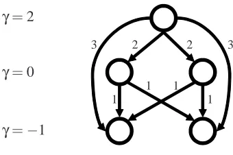
label y is more relevant to the instance than label y′. The preferences over the labels can also be described as a weighted directed graph: the nodes of the graph are the labels and weighted edges encode pairwise preferences over pairs of labels. In Fig. 1 we give the graph representation for the target vector(−1,0,2,0,−1)where each edge marked with its weight. For instance, the weight of the edge(3,1)isγ3−γ1=3.

The class of mappings we employ in this paper is the set of linear functions. While this func-tion class may seem restrictive, the pioneering work of Vapnik (1998) and colleagues demonstrates that by using Mercer kernels one can employ highly non-linear predictors, called support vector machines (SVM) and still entertain all the formal properties and simplicity of linear predictors. We propose a SVM-like learning paradigm for predicting the preferences over labels. We generalize the definition of the hinge-loss used in SVM to the label ranking setting. Our generalized hinge loss contrasts the predicted preferences graph and the target preferences graph by decomposing the target graph into bipartite sub-graphs. As we discuss in the next section, this decomposition into sub-graphs is rather flexible and enables us to analyze several previously defined loss functions in a single unified setting. This definition of the generalized hinge loss lets us pose the learning problem as a quadratic optimization problem while the structured decomposition leads to an efficient and effective optimization procedure.

The main building block of our optimization procedure is an algorithm which performs fast and frugalSOftProjectionsOnto aPOlyhedron and is therefore abbreviated SOPOPO. Generalizing the iterative algorithm proposed by Hildreth (1957) (see also Censor and Zenios (1997)) from half-space constraints to polyhedra constraints, we also derive and analyze an iterative algorithm which on each iteration performs a soft projection onto a single polyhedron. The end result is a fast optimization procedure for label ranking from general real-valued feedback.

The paper is organized as follows. In Sec. 2 we start with a formal definition of our setting and cast the learning task as a quadratic programming problem. We also make references to previous work on related problems that are covered by our setting. Our efficient optimization procedure for the resulting quadratic problem is described in two steps. First, we present in Sec. 3 the SOPOPO algorithm for projecting onto a single polyhedron. Then, in Sec. 4, we derive and analyze an iterative algorithm which solves the original quadratic optimization problem by successive activations of SOPOPO. Experiments are provided in Sec. 5 and concluding remarks are given in Sec. 6.

γ=2

γ=0

γ=−1

3 2 2 3

1 1

1 1

Figure 1: The graph induced by the feedbackγ= (−1,0,2,0,−1).

2. Problem Setting

In this section we introduce the notation used throughout the paper and formally describe our prob-lem setting. We denote scalars with lower case letters (e.g. x and α), and vectors with bold face letters (e.g. x andα). Sets are designated by upper case Latin letters (e.g. E) and set of sets by bold face (e.g. E). The set of non-negative real numbers is denoted byR+. For any k≥1, the set of integers{1, . . . ,k}is denoted by[k]. We use the notation(a)₊to denote the hinge function, namely,

(a)₊=max{0,a}.

Let

X

be an instance domain and let

Y

= [k]be a predefined set of labels. A target for an instance x∈

X

is a vectorγ∈Rkwhereγy>γy′ means that y is more relevant to x than y′. We also

refer toγas a label ranking. We would like to emphasize that two different labels may attain the same rank, that is,γy=γy′ while y6=y′. In this case, we say that y and y′are of equal relevance to

x. We can also describeγas a weighted directed graph. The nodes of the graph are labeled by the elements of[k]and there is a directed edge of weightγr−γsfrom node r to node s iffγr>γs. In Fig. 1 we give the graph representation for the label-ranking vectorγ= (−1,0,2,0,−1).

The learning goal is to learn a ranking function of the form f :

X

→Rk which takes x as an input instance and returns a ranking vector f(x)∈Rk. We denote by fr(x)the rth element of f(x). Analogous to the target vector,γ, we say that label y is more relevant than label y′with respect to the predicted ranking if fy(x)> fy′(x). We assume that the label-ranking functions are linear, namely,

fr(x) =wr·x ,

where each wr is a vector in Rn and

X

⊆Rn. As we discuss briefly at the end of Sec. 4, our al-gorithm can be generalized straightforwardly to non-linear ranking functions by employing Mercer kernels (Vapnik, 1998).

We focus on a batch learning setting in which a training set S={(xi_,γi_)}m

with respect to the pair as,

ℓr,s(f(x),γ) = ((γr−γs)−(fr(x)−fs(x)))+ . (1)

The above definition of loss extends the hinge-loss used in binary classification problems (Vapnik, 1998) to the problem of label-ranking. The lossℓr,s reflects the amount by which the constraint

fr(x)−fs(x)≥γr−γs is not satisfied. While the construction above is defined for pairs, our goal though is to associate a loss with the entire predicted ranking and not a single pair. Thus, we need to combine the individual losses over pairs into one meaningful loss. In this paper we take a rather flexible approach by specifying an apparatus for combining the individual losses over pairs into a single loss. We combine the different pair-based losses into a single loss by grouping the pairs of labels into independent sets each of which is isomorphic to a complete bipartite graph. Formally, given a target label-ranking vector γ∈Rk, we define E(γ) ={E1, . . . ,Ed} to be a collection of subsets of

Y

×

Y

. For each j∈[d], define Vjto be the set of labels which support the edges in Ej, that is,

Vj={y∈

Y

:∃r s.t.(r,y)∈Ej∨(y,r)∈Ej} . (2) We further require that E(γ)satisfies the following conditions,

1. For each j∈[d]and for each(r,s)∈Ejwe haveγr>γs.

2. For each i6= j∈[d]we have Ei∩Ej=/0.

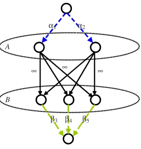
3. For each j∈[d], the sub-graph defined by(Vj,Ej)is a complete bipartite graph. That is, there exists two sets A and B, such that A∩B=/0, Vj=A∪B, and Ej=A×B.

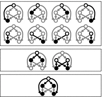
In Fig. 2 we illustrate a few possible decompositions into bipartite graphs for a given label-ranking. The loss of each sub-graph (Vj,Ej) is defined as the maximum over the losses of the pairs belonging to the sub-graph. In order to add some flexibility we also allow different sub-graphs to have different contribution to the loss. We do so by associating a weightσj with each sub-graph. The general form of our loss is therefore,

ℓ(f(x),γ) =

d

∑

j=1

σj max

(r,s)∈Ej

ℓr,s(f(x),γ) , (3)

where eachσj∈R+is a non-negative weight. The weightsσjcan be used to associate importance values with each sub-graph(Vj,Ej) and to facilitate different notions of losses. For example, in multilabel classification problems, each instance is associated with a set of relevant labels which come from a predefined set

Y

. The multilabel classification problem is a special case of the label ranking problem discussed in this paper and can be realized by setting γr=1 if the r’th label is relevant and otherwise defining γr=0. Thus, the feedback graph itself is of a bipartite form. Its edges are from A×B where A consists of all the relevant labels and B of the irrelevant ones. If

we decide to set E(γ) to contain the single set A×B and define σ1=1 then ℓ(f(x),γ) amounts to the maximum value ofℓr,s over pairs of edges in A×B. Thus, the loss of this decomposition distills to the worst loss suffered over all pairs of comparable labels. Alternatively, we can set E(γ)

Figure 2: Three possible decompositions into complete bipartite sub-graphs of the graph from Fig. 1. Top: all-pairs decomposition; Middle: all adjacent layers; Bottom: top layer versus the rest of the layers. The edges and vertices participating in each sub-graph are depicted in black while the rest are presented in gray. In each graph the nodes constituting the set A are designated by black circles while for the nodes in B by filled black circles.

can thus capture different notions of losses for label ranking functions with multitude schemes for casting the relative importance of each subset(Vj,Ej).

Equipped with the loss function given in Eq. (3) we now formally define our learning problem. As in most learning settings, we assume that there exists an unknown distribution D over

X

×Rk

and that each example in our training set is identically and independently drawn from D. The ultimate goal is to learn a label ranking function f which entertains a small generalization loss,

term and the empirical loss term is controlled by a parameter C. The resulting optimization problem is,

min w1,...,wk

1 2

k

∑

j=1

kwjk2 +C m

∑

i=1

ℓ(f(xi),γi) , (4)

where fy(xi) =wy·xi. Note that the loss function in Eq. (3) can also be represented as the solution of the following optimization problem,

ℓ(f(x),γ) = min

ξ∈Rd

+ d

∑

j=1 σj ξj

s.t. ∀j∈[d], ∀(r,s)∈Ej, fr(x)−fs(x)≥γr−γs−ξj ,

(5)

where d=|E(γ)|. Thus, we can rewrite the optimization problem given in Eq. (4) as a quadratic optimization problem,

min w1,...,wk,ξ

1 2

k

∑

j=1

kwjk2 +C m

∑

i=1

|E(γi_)|

∑

j=1 σjξij

s.t. ∀i∈[m],∀Ej∈E(γi), ∀(r,s)∈Ej, wr·xi−ws·xi≥γir−γis−ξij

∀i,j, ξi j≥0 .

(6)

To conclude this section, we would like to review the rationale for choosing an one-sided loss for each pair by casting a single inequality for each (r,s). It is fairly easy to define a two-sided loss for a pair by mimicking regression problems. Concretely, we could replace the definition of

ℓr,sas given in Eq. (1) with the loss|fr(x)−fs(x)−(γr−γs)|. This loss penalizes for any deviation from the desired difference of γr−γs. Instead, our loss is one sided as it penalizes only for not achieving a lower-bound. This choice is more natural in ranking applications. For instance, suppose we need to induce a ranking over 4 labels where the target label ranking is(−1,2,0,0). Assume that the predicted ranking is instead(−5,3,0,0). In most ranking and search applications such a predicted ranking would be perceived as being right on target since the preferences it expresses over pairs are on par with the target ranking. Furthermore, in most ranking applications, overly demotion of the most irrelevant items and excessive promotion of the most relevant ones is perceived as beneficial rather than a deficiency. Put another way, the set of target values encode minimal margin requirements and over-achieving these margin requirements should not be penalized.

While the learning algorithms from (Weston and Watkins, 1999) and (Crammer and Singer, 2001) are seemingly different, they can be solved using the same algorithmic infrastructure presented in this paper. Proceeding to more complex decision problems, the task of multilabel classification or ranking is concerned with predicting a set or relevant labels or ranking the labels in accordance to their relevance to the input instance. This problem was studied by several authors (Elisseeff and Weston, 2001; Crammer and Singer, 2002; Dekel et al., 2003). Among these studies, the work of Elisseeff and Weston (2001) is probably the closest to ours yet it is still a derived special case of our setting . Elisseeff and Weston focus on a feedback vector γ which constitutes a bipartite graph by itself and define a constrained optimization problem with a separate slack variable for each edge in the graph. Formally, each instance x is associated with a set of relevant labels denoted

Y . As discussed in the example above, the multilabel categorization setting can thus be realized by

definingγr=1 for all r∈Y andγs=0 for all s6∈Y . The construction of Elisseeff and Weston can be recovered by defining E(γ) ={{(r,s)}|γr>γs}. Our approach is substantially more general as it allows much richer and flexible ways to decompose the multilabel problem as well as more general label ranking problems.

3. Fast “Soft” Projections

In the previous section we introduced the learning apparatus. Our goal now is to derive and analyze an efficient algorithm for solving the label ranking problem. In addition to efficiency, we also require that the algorithm would be general and flexible so it can be used with any decomposition of the feedback according to E(γ). While the algorithm presented in this and the coming sections is indeed efficient and general, its derivation is rather complex. We therefore would like to present it in a bottom-up manner starting with a sub-problem which constitutes the main building block of the algorithm. In this sub-problem we assume that we have obtained a label-ranking function realized by the set u1, . . . ,ukand the goal is to modify the ranking function so as to fit better a newly obtained example. To further simplify the derivation, we focus on the case where E(γ)contains a single complete bipartite graph whose set of edges are simply denoted by E. The end result is the following simplified constrained optimization problem,

min w1,...,wk,ξ

1 2

k

∑

y=1

kwy−uyk2+Cξ

s.t. ∀(r,s)∈E, wr·x−ws·x≥γr−γs−ξ ξ≥0 .

(7)

Here x∈

X

is a single instance and E is a set of edges which induces a complete bipartite graph. The focus of this section is an efficient algorithm for solving Eq. (7). This optimization problem finds the set closest to {u1, . . . ,uk} which approximately satisfies a system of linear constraints with a single slack (relaxation) variableξ. Put another way, we can view the problem as the task of finding a relaxed projection of the set {u1, . . . ,uk} onto the polyhedron defined by the set of linear constraints induced from E. We thus refer to this task as the soft projection. Our algorithmic solution, while being efficient, is rather detailed and its derivation consists of multiple complex steps. We therefore start with a high level overview of its derivation. We first derive a dual version of the problem defined by Eq. (7). Each variable in the dual problem corresponds to an edge in

and more compact optimization problem which has only k variables. We prove that the reduced problem nonetheless attains the same optimum as the original dual problem. This reduction is one of the two major steps in the derivation of an efficient soft projection procedure. We next show that the reduced problem can be decoupled into two simpler constrained optimization problems each of which corresponds to one layer in the bipartite graph induced by E. The two problems are tied by a single variable. We finally reach an efficient solution by showing that the optimal value of the coupling variable can be efficiently computed in O(k log(k))time. We recap our entire derivation by providing the pseudo-code of the resulting algorithm at the end of the section.

3.1 The Dual Problem

To start, we would like to note that the primal objective function is convex and all the primal con-straints are linear. A necessary and sufficient condition for strong duality to hold in this case is that there exists a feasible solution to the primal problem (see for instance (Boyd and Vandenberghe, 2004)). A feasible solution can indeed obtained by simply setting wy =0 for all y and defining ξ=max(r,s)∈E(γr−γs). Therefore, strong duality holds and we can obtain a solution to the primal problem by finding the solution of its dual problem. To do so we first write the Lagrangian of the primal problem given in Eq. (7), which amounts to,

L

= 1

2 k

∑

y=1

kwy−uyk2+Cξ+

∑

(r,s)∈E

τr,s(γr−γs−ξ+ws·x−wr·x)−ζξ

= 1

2 k

∑

y=1

kwy−uyk2+ξ C−

∑

(r,s)∈E τr,s−ζ

!

+

∑

(r,s)∈E

τr,s(γr−wr·x−γs+ws·x) ,

whereτr,s≥0 for all (r,s)∈E andζ≥0. To derive the dual problem we now can use the strong duality. We eliminate the primal variables by minimizing the Lagrangian with respect to its primal variables. First, note that the minimum of the termξ(C−∑_(r,s)∈Eτr,s−ζ)with respect toξis zero whenever C−∑_(r,s)∈Eτr,s−ζ=0. If however C−∑(r,s)∈Eτr,s−ζ6=0 then this term can be made to approach−∞. Since we need to maximize the dual we can rule out the latter case and pose the following constraint on the dual variables,

C−

∑

(r,s)∈E

τr,s−ζ = 0 . (8)

Next, recall our assumption that E induces a complete bipartite graph (V,E) (see also Eq. (2)). Therefore, there exists two sets A and B such that A∩B=/0, V =A∪B, and E=A×B. Using the

definition of the sets A and B we can rewrite the last sum of the Lagrangian as,

∑

r∈A,s∈B

τr,s(γr−wr·x−γs+ws·x) =

∑

r∈A

(γr−wr·x)

∑

s∈B

τr,s −

∑

s∈B

(γs−ws·x)

∑

r∈A

τr,s .

Eliminating the remaining primal variables w1, . . . ,wk is done by differentiating the Lagrangian with respect to wrfor all r∈[k]and setting the result to zero. For all y∈A, the above gives the set of constraints,

∇wy

L

= wy−uy−

∑

s∈B

τy,s

!

Similarly, for y∈B we get that,

∇wy

L

= wy−uy+

∑

r∈A

τr,y

!

x = 0 . (10)

Finally, we would like to note that for any label y∈/A∪B we get that wy−uy=0. Thus, we can omit all such labels from our derivation. Summing up, we get that,

wy =

 



uy+ (∑s∈Bτy,s)x y∈A uy−(∑r∈Aτr,y)x y∈B uy otherwise

. (11)

Plugging Eq. (11) and Eq. (8) into the Lagrangian and rearranging terms give the following dual objective function,

D(τ) = −1

2kxk 2

∑

y∈A s

∑

∈B τy,s

!2

−1

2kxk 2

∑

y∈B r

∑

∈A τr,y

!2

(12)

+

∑

y∈A

(γy−uy·x)

∑

s∈B

τy,s−

∑

y∈B

(γy−uy·x)

∑

r∈A

τr,y .

In summary, the resulting dual problem is,

max

τ∈R|+E|

D(τ) s.t.

∑

(r,s)∈E

τr,s≤C . (13)

3.2 Reparametrization of the Dual Problem

Each dual variable τr,s corresponds to an edge in E. Thus, the number of dual variables may be as large as k2/4. However, the dual objective function depends only on sums of variables τr,s.

Furthermore, each primal vector wy also depends on sums of dual variables (see Eq. (11)). We exploit these useful properties to introduce an equivalent optimization of a smaller size with only k variables. We do so by defining the following variables,

∀y∈A, αy=

∑

s∈B

τy,s and ∀y∈B, βy=

∑

r∈A

τr,y . (14)

The primal variables wyfrom Eq. (11) can be rewritten usingαyandβy as follows,

wy =

 



uy+αyx y∈A uy−βyx y∈B uy otherwise

. (15)

Overloading our notation and using D(α,β)to denote dual objective function in terms ofαandβ, we can rewrite the dual objective of Eq. (12) as follows,

D(α,β) =−1

2kxk

2

∑

y∈A α2

y+

∑

y∈B

β2 y

!

+

∑

y∈A

(γy−uy·x)αy −

∑

y∈B

Note that the definition ofαyandβyfrom Eq. (14) implies thatαyandβyare non-negative. Further-more, by construction we also get that,

∑

y∈A

αy =

∑

y∈B

βy =

∑

(r,s)∈E

τr,s ≤ C . (17)

In summary, we have obtained the following constrained optimization problem,

max

α∈R|+A|,β∈R|+B|

D(α,β) s.t.

∑

y∈A

αy=

∑

y∈B

βy≤C . (18)

We refer to the above optimization problem as the reduced problem since it encompasses at most k=|V|variables. In appendix A we show that the reduced problem and the original dual problem from Eq. (13) are equivalent. The end result is the following corollary.

Corollary 1 Let(α⋆,β⋆)be the optimal solution of the reduced problem in Eq. (18). Define{w1, . . . ,wk}

as in Eq. (15). Then,{w1, . . . ,wk}is the optimal solution of the soft projection problem defined by

Eq. (7).

We now move our focus to the derivation of an efficient algorithm for solving the reduced problem. To make our notation easy to follow, we define p=|A|and q=|B|and construct two vectors µ∈Rp andν∈Rq such that for each a∈A there is an element(γa−ua·x)/kxk2 in µ and for each b∈B there is an element−(γb−ub·x)/kxk2inν. The reduced problem can now be rewritten as,

min

α∈R+p,β∈R

q +

1

2kα−µk 2₊1

2kβ−νk 2

s.t. p

∑

i=1 αi =

q

∑

j=1

βj ≤ C .

(19)

3.3 Decoupling the Reduced Optimization Problem

In the previous section we showed that the soft projection problem given by Eq. (7) is equivalent to the reduced optimization problem of Eq. (19). Note that the variablesαandβare tied together through a single equality constraintkαk1=kβk1. We represent this coupling ofαandβby rewriting the optimization problem in Eq. (19) as,

min

z∈[0,C] g(z; µ) +g(z;ν) ,

where

g(z; µ) = min

α

1

2kα−µk 2 _s.t.

p

∑

i=1

αi = z, αi≥0 , (20)

and similarly

g(z;ν) = min

β

1

2kβ−νk 2 _s.t.

q

∑

j=1

The function g(z;·)takes the same functional form whether we use µ orνas the second argument. We therefore describe our derivation in terms of g(z; µ). Clearly, the same derivation is also appli-cable to g(z;ν). The Lagrangian of g(z; µ)is,

L

= 1

2kα−µk

2_+θ

∑

p i=1

αi−z

!

−ζ·α ,

whereθ∈Ris a Lagrange multiplier andζ∈R+p is a vector of non-negative Lagrange multipliers.

Differentiating with respect toαiand comparing to zero gives the following KKT condition,

dL dαi

= αi−µi+θ−ζi = 0 .

The complementary slackness KKT condition implies that whenever αi >0 we must have that ζi=0. Thus, ifαi>0 we get that,

αi = µi−θ+ζi = µi−θ . (22)

Since all the non-negative elements of the vectorα are tied via a single variable we would have ended with a much simpler problem had we known the indices of these elements. On a first sight, this task seems difficult as the number of potential subsets ofα is clearly exponential in the di-mension ofα. Fortunately, the particular form of the problem renders an efficient algorithm for identifying the non-zero elements ofα. The following lemma is a key tool in deriving our proce-dure for identifying the non-zero elements.

Lemma 2 Letαbe the optimal solution to the minimization problem in Eq. (20). Let s and j be two indices such that µs>µj. Ifαs=0 thenαj must be zero as well.

Proof Assume by contradiction thatαs=0 yetαj>0. Let ˜α∈Rk be a vector whose elements are equal to the elements ofαexcept for ˜αsand ˜αj which are interchanged, that is, ˜αs=αj, ˜αj =αs, and for every other r∈ {s/ ,j} we have ˜αr=αr. It is immediate to verify that the constraints of Eq. (20) still hold. In addition we have that,

kα−µk2− kα˜ −µk2 = µ2_s+ (αj−µj)2−(αj−µs)2−µ2j = 2αj(µs−µj) > 0 .

Therefore, we obtain that kα−µk2 _>kα_˜−µk2_{, which contradicts the fact that} α _{is the optimal} solution.

Let I denote the set{i∈[p]:αi>0}. The above lemma gives a simple characterization of the set

I. Let us reorder the µ such that µ1≥µ2≥. . .≥µp. Simply put, Lemma 2 implies that after the reordering, the set I is of the form{1, . . . ,ρ}for some 1≤ρ≤p. Had we knownρwe could have simply use Eq. (22) and get that

p

∑

i=1 αi=

ρ

∑

i=1 αi=

ρ

∑

i=1

(µi−θ) =z ⇒ θ= 1 ρ

ρ

∑

i=1

µi−z

!

.

In summary, givenρwe can summarize the optimal solution forαas follows,

αi =

  

 

µi− 1 ρ

ρ

∑

i=1

µi−z

!

i≤ρ

0 i>ρ

We are left with the problem of finding the optimal value of ρ. We could simply enumerate all possible values ofρin[p], for each possible value computeαas given by Eq. (23), and then choose the value for which the objective function (kα−µk2_{) is the smallest. While this procedure can} be implemented quite efficiently, the following lemma provides an even simpler solution once we reorder the elements of µ to be in a non-increasing order.

Lemma 3 Letαbe the optimal solution to the minimization problem given in Eq. (20) and assume that µ1≥µ2≥. . .≥µp. Then, the number of strictly positive elements inαis,

ρ(z,µ) = max

(

j∈[p] : µj− 1

j

j

∑

r=1

µr−z

!

>0

)

.

The proof of this technical lemma is deferred to the appendix.

Had we known the optimal value of z, i.e. the argument attaining the minimum of g(z; µ) + g(z;ν) we could have calculated the optimal dual variablesα⋆ andβ⋆ by first findingρ(z,µ)and ρ(z,ν)and then findingα andβusing Eq. (23). This is a classical chicken-and-egg problem: we can easily calculate the optimal solution given some side information, however, obtaining the side information seems as difficult as finding the optimal solution. One option is to perform a search over anε-net of values for z in[0,C]. For each candidate value for z from theε-net we can findα andβand then choose the value which attains the lowest objective value (g(z; µ) +g(z;ν)). While this approach may be viable in many cases, it is still quite time consuming. To our rescue comes the fact that g(z; µ) and g(z;ν)entertain a very special structure. Rather than enumerating over all possible values of z we need to check at most k+1 possible values for z. To establish the last part of our efficient algorithm which performs this search for the optimal value of z we need the following theorem. The theorem is stated with µ but, clearly, it also holds forν.

Theorem 4 Let g(z; µ)be as defined in Eq. (20). For each i∈[p], define

zi= i

∑

r=1

µr−iµi .

Then, for each z∈[zi,zi+1]the function g(z; µ)is equivalent to the following quadratic function,

g(z; µ) = 1 i

i

∑

r=1

µr−z

!2

+

p

∑

r=i+1

µ2_r .

Moreover, g is continuous, continuously differentiable, and convex in[0,C].

The proof of this theorem is also deferred to the appendix. The good news that the theorem carries is that g(z; µ)and g(z;ν)are convex and therefore their sum is also convex. Furthermore, the function

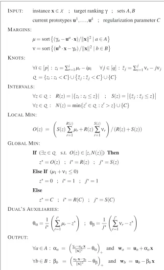
INPUT: instance x∈

X

; target rankingγ ; sets A,B

current prototypes u1, . . . ,uk ; regularization parameter C MARGINS:

µ=sort(γa−ua·x)/kxk2|a∈A ν=sort(ub·x−γb)/kxk2|b∈B KNOTS:

∀i∈[p]: zi=∑ir=1µr−iµi ∀j∈[q]: ˜zj=∑sj=1νs−jνj

Q

={zi: zi<C} ∪

˜zj: ˜zj<C ∪ {C} INTERVALS:

∀z∈

Q

: R(z) =|{zi: zi≤z}| ; S(z) =

{˜zj: ˜zj≤z}

∀z∈

Q

: N(z) =min{z′∈

Q

: z′>z} ∪ {C}

LOCALMIN:

O(z) = S(z)

R(z)

∑

r=1

µr+R(z) S(z)

∑

r=1 νr

!

/(R(z) +S(z))

GLOBALMIN:

If (∃z∈

Q

s.t. O(z)∈[z,N(z)]) Then

z⋆=O(z) ; i⋆=R(z) ; j⋆=S(z)

Else If (µ1+ν1≤0)

z⋆=0 ; i⋆=1 ; j⋆=1

Else

z⋆=C ; i⋆=R(C) ; j⋆=S(C)

DUAL’SAUXILIARIES:

θα= 1 i⋆

i⋆

∑

r=1

µr−z⋆

!

; θ_β= 1 j⋆

j⋆

∑

r=1 νr−z⋆

!

OUTPUT:

∀a∈A : αa =

_γ

a−ua·x

kxk2 −θα

+ and wa = ua+αax ∀b∈B : βb =

ub·x−γb

kxk2 −θβ

+ and wb = ub−βbx

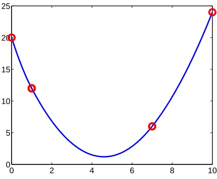
0 2 4 6 8 10 0

5 10 15 20 25

Figure 4: An illustration of the function g(z; µ) +g(z;ν). The vectors µ andνare constructed from, γ= (1,2,3,4,5,6), u·x= (2,3,5,1,6,4), A={4,5,6}, and B={1,2,3}.

3.4 Putting it All Together

Due to the strict convexity of g(z; µ) +g(z;ν)its minimum is unique and well defined. Therefore, it suffices to search for a seemingly local minimum over all the sub-intervals in which the objective function is equivalent to a quadratic function. If such a local minimum point is found it is guaranteed to be the global minimum. Once we have the value of z which constitutes the global minimum we can decouple the optimization problems forα andβand quickly find the optimal solution. There is though one last small obstacle: the objective function is the sum of two piecewise quadratic functions. We therefore need to efficiently go over the union of the knots derived from µ andν. We now summarize the full algorithm for finding the optimum of the dual variables and wrap up with its pseudo-code.

Given µ andνwe find the sets of knots for each vector, take the union of the two sets, and sort the set in an ascending order. Based on the theorems above, it follows immediately that each interval between two consecutive knots in the union is also quadratic. Since g(z; µ) +g(z;ν)is convex, the objective function in each interval can be characterized as falling into one of two cases. Namely, the objective function is either monotone (increasing or decreasing) or it attains its unique global minimum inside the interval. In the latter case the objective function clearly decreases, reaches the optimum where its derivative is zero, and then increases. See also Fig. 4 for an illustration. If the objective function is monotone in all of the intervals then the minimum is obtained at one of the boundary points z=0 or z=C. Otherwise, we simply need to identify the interval bracketing

We utilize the following notation. For each i∈[p], define the knots derived from µ

zi= i

∑

r=1

µr−iµi ,

and similarly, for each j∈[q]define

˜zj= j

∑

r=1

νr−jνj .

From Lemma 4 we know that g(z; µ)is quadratic in each segment[zi,zi+1)and g(z;ν)is quadratic in each segment[˜zj,˜zj+1). Therefore, as already argued above, the function g(z; µ) +g(z;ν)is also piecewise quadratic in[0,C]and its knots are the points in the set,

Q

={zi: zi<C} ∪ {˜zj: ˜zj<C} ∪ {C} .

For each knot z∈

Q

, we denote by N(z)its consecutive knot in

Q

, that is,

N(z) =min {z′∈

Q

: z′>z} ∪ {C} .

We also need to know for each knot how many knots precede it. Given a knot z we define

R(z) =|{zi: zi≤z}| and S(z) =|{˜zi: ˜zi≤z}| .

Using the newly introduced notation we can find for a given value z its bracketing interval, z∈ [z′,N(z′)]. From Thm. 4 we get that the value of the dual objective function at z is,

g(z; µ) +g(z;ν) =

1

R(z′₎

R(z′)

∑

r=1

µr−z

!2

+

p

∑

r=R(z′₎₊₁

µ2_r+ 1 S(z′₎

S(z′)

∑

r=1 νr−z

!2

+

p

∑

r=S(z′₎₊₁

ν2 r .

The unique minimum of the quadratic function above is attained at the point

O(z′) = S(z′)

R(z′)

∑

i=1

µi+R(z′) S(z′)

∑

i=1 νi

!

/ R(z′) +S(z′) .

Therefore, if O(z′)∈[z′,N(z′)], then the global minimum of the dual objective function is attained at O(z′). Otherwise, if no such interval exists, the optimum is either at z=0 or at z=C. The

4. From a Single Projection to Multiple Projections

We now describe the algorithm for solving the original batch problem defined by Eq. (6) using the SOPOPO algorithm as its core. We would first like to note that the general batch problem can also be viewed as a soft projection problem. We can cast the batch problem as finding the set of vectors{w1, . . . ,wk}which is closest to k zero vectors{0, . . . ,0}while approximately satisfying a set of systems of linear constraints where each system is associated with an independent relaxation variable. Put another way, we can view the full batch optimization problem as the task of finding a relaxed projection of the set {0, . . . ,0} onto multiple polyhedra each of which is defined via a set of linear constraints induced by a single sub-graph Ej ∈E(γi_{). We thus refer to this task as the} soft-projection onto multiple polyhedra. We devise an iterative algorithm which solves the batch problem by successively calling to the SOPOPO algorithm from Fig. 3. We describe and analyze the algorithm for a slightly more general constrained optimization which results in a simplified notation. We start with the presentation of our original formulation as an instance of the generalized problem.

To convert the problem in Eq. (6) to a more general form, we assume without loss of generality that|E(γi_{)|=1 for all i∈[m]. We refer to the single set in E(γ}i_{)as E}i_{. This assumption does not} pose a limitation since in the case of multiple decompositions, E(γi_{) ={E}

1, . . . ,Ed}, we can replace the ith example with d pseudo-examples: {(xi,E1), . . . ,(xi,Ed)}. Using this assumption, we can rewrite the optimization problem of Eq. (6) as follows,

min w1,...,wk,ξ

1 2

k

∑

r=1

kwrk2 + m

∑

i=1

Ciξi

s.t. ∀i∈[m],∀(r,s)∈Ei, wr·xi−ws·xi≥γir−γis−ξi

∀i, ξi≥0 ,

(24)

where Ci=Cσiis the weight of the ith slack variable. To further simplify Eq. (24), we use ¯w∈Rnk to denote the concatenation of the vectors(w1, . . . ,wk). In addition, we associate an index, denoted

j, with each(r,s)∈Eiand define ai,j∈Rnk to be the vector, ai,j= ( 0

|{z}

1st block

, . . . , 0, xi

|{z}

rth block

,0, , . . . ,0, −xi

|{z}

sth block

,0, . . . , 0

|{z}

kth block

) . (25)

We also define bi,j=γi

r−γis. Finally, we define ki=|Ei|. Using the newly introduced notation we can rewrite Eq. (24) as follows,

min ¯ w,ξ

1 2kw¯k

2₊

∑

m i=1

Ciξi

s.t. ∀i∈[m],∀j∈[ki], w¯ ·ai,j≥bi,j−ξi ξi_{≥0 .}

(26)

Our goal is to derive an iterative algorithm for solving Eq. (26) based on a procedure for solving a single soft-projection which takes the form,

min ¯ w,ξi

1

2kw¯ −uk 2_+C

iξi

s.t. ∀j∈[ki], w¯ ·ai,j≥bi,j−ξi ξi_{≥0 .}

By construction, an algorithm for solving the more general problem defined in Eq. (26) would also solve the more specific problem defined by Eq. (6).

The rest of the section is organized as follows. We first derive the dual of the problem given in Eq. (26). We then describe an iterative algorithm which on each iteration performs a single soft-projection and present a pseudo-code of the iterative algorithm tailored for the specific label-ranking problem of Eq. (6). Finally, we analyze the convergence of the suggested iterative algorithm.

4.1 The Dual Problem

First, note that the primal objective function of the general problem is convex and all the primal constraints are linear. Therefore, using the same arguments as in Sec. 3.1 it is simple to show that strong duality holds and a solution to the primal problem can be obtained from the solution of its dual problem. To derive the dual problem, we first write the Lagrangian,

L

= 1

2kw¯k 2₊

∑

m

i=1

Ciξi+ m

∑

i=1 ki

∑

j=1

λi,j bi,j−ξi−w¯ ·ai,j

−

m

∑

i=1 ζiξi ,

whereλi,jandζi are non-negative Lagrange multipliers. Taking the derivative of

L

with respect to ¯

w and comparing it to zero gives,

¯ w =

m

∑

i=1 ki

∑

j=1

λi,jai,j . (28)

As in the derivation of the dual objective function for a single soft projection, we get that the following must hold at the optimum,

∀i∈[m],

ki

∑

j=1

λi,j−Ci−ζi=0 . (29)

Sinceλi,j andζi are non-negative Lagrange multipliers we get that the set of feasible solutions of the dual problem is,

S = ( λ ∀i, ki

∑

j=1

λi,j ≤ Ci and ∀i,j,λi,j≥0

)

.

Using Eq. (28) and Eq. (29) to further rewrite the Lagrangian gives the dual objective function,

D(λ) = −1

2 m

∑

i=1 ki

∑

j=1 λi,jai,j

2 + m

∑

i=1 ki

∑

j=1

λi,jbi,j .

The dual of the problem defined in Eq. (26) is therefore,

max

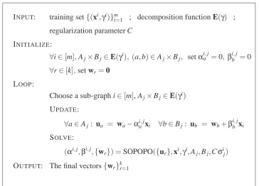
INPUT: training set{(xi,γi_)}m

i=1 ; decomposition function E(γ) ; regularization parameter C

INITIALIZE:

∀i∈[m],Aj×Bj∈E(γi), (a,b)∈Aj×Bj, setαai,j=0,βi_b,j=0

∀r∈[k],set wr=0 LOOP:

Choose a sub-graph i∈[m], Aj×Bj∈E(γi) UPDATE:

∀a∈Aj: ua = wa−αia,jxi ∀b∈Bj: ub = wb+βi_b,jxi SOLVE:

(αi,j,βi,j,{wr}) =SOPOPO({ur},xi,γi,Aj,Bj,Cσij)

OUTPUT: The final vectors{wr}kr=1

Figure 5: The procedure for solving the preference graphs problem via soft-projections.

4.2 An Iterative Procedure

We are now ready to describe our iterative algorithm. We would like to stress again that the method-ology and analysis presented here have been suggested by several authors. Our procedure is a slight generalization of row action methods (Censor and Zenios, 1997) which is often referred to as de-composition methods (see also Lin (2002); Mangasarian and Musicant (1999); Platt (1998)). The iterative procedure works in rounds and operates on the dual form of the objective function. We show though that each round can be realized as a soft-projection operation. Letλt denote the vector of dual variables before the tth iteration of the iterative algorithm. Initially, we setλ1=0, which constitutes a trivial feasible solution to Eq. (30). On the tth iteration of the algorithm, we choose a single example whose index is denoted r and update its dual variables. We freeze the rest of the dual variables at their current value. We cast the tth iteration as the following constrained optimization problem,

λt+1 _{= argmax}

λ∈S

D(λ) s.t. ∀i6=r,∀j∈[ki], λi,j=λti,j . (31)

Note thatλt+1is essentially the same asλtexcept for the variables corresponding to the rth example, namely,{λr,j|j∈[kr]}. In order to explicitly write the objective function conveyed by Eq. (31) let us introduce the following notation,

u =

∑

i6=r ki

∑

j=1 λt

The vector u is equal to the current estimate of ¯w excluding the contribution of the rth set of dual variables. With u on hand, we can rewrite the objective function of Eq. (31) as follows,

− 1 2 kr

∑

j=1 λr,jar,j

2 − kr

∑

j=1 λr,jar,j

!

·u−1

2kuk 2₊

∑

kr

j=1

λr,jbr,j+

∑

i6=r

ki

∑

j=1 λt

i,jbi,j

=−1

2 kr

∑

j=1 λr,jar,j

2 + kr

∑

j=1

λr,j br,j−u·ar,j

+Γ , (33)

whereΓis a constant that does not depend on the variables in{λr,j|j∈[kr]}. In addition the set of variables which are not fixed must reside in S, therefore,

ki

∑

j=1

λr,j ≤ Cr and ∀j,λr,j≥0 . (34)

The fortunate circumstances are that the optimization problem defined by Eq. (33) subject to the constraints given in Eq. (34) can be rephrased as a soft-projection problem. Concretely, let us define the following soft-projection problem,

min ¯ w,ξr

1

2kw¯ −uk 2_+C

rξr

s.t. ∀j∈[kr], w¯ ·ar,j≥br,j−ξr ξr_{≥0 .}

(35)

The value ofλt_r+_,j1 is obtained from the optimal value of the dual problem of Eq. (35) as we now show. The Lagrangian of Eq. (35) is

L

= 1

2kw¯ −uk 2_+C

rξr+ kr

∑

j=1

λr,j br,j−ξr−w¯ ·ar,j

−ζrξr .

Differentiating with respect to ¯w and comparing to zero give,

¯

w = u+

kr

∑

j=1

λr,jar,j .

As in the previous derivations of the dual objective functions we also get that,

Cr−ζr− kr

∑

j=1

λr,j = 0 ,

and thus the Lagrange multipliers must satisfy,

kr

∑

j=1

Therefore, the dual problem of Eq. (35) becomes,

max

λr,·

−1

2

kr

∑

j=1 λr,jar,j

2

+

kr

∑

j=1

λr,j(br,j−u·ar,j) s.t.

kr

∑

j=1

λr,j≤Cr and ∀j,λr,j≥0 ,

(36)

which is identical to the problem defined by Eq. (33) subject to the constraints given by Eq. (34). In summary, our algorithm works by updating one set of dual variables on each round while fixing the rest of the variables to their current values. Finding the optimal value of the unrestricted variables is achieved by defining an instantaneous projection problem. The instantaneous soft-projection problem is readily solved using the machinery developed in the previous section. The pseudo-code of this iterative procedure is given in Fig. 5. It is therefore left to reason about the formal properties of the iterative procedure. From the definition of the update from Eq. (31) we clearly get that on each round we are guaranteed to increase the dual objective function unless we are already at the optimum. In the next subsection we show that this iterative paradigm converges to the global optimum of the dual objective function.

To conclude this section, we would like to note that a prediction of our label-ranking function is solely based on inner products between vectors from{w1, . . . ,wk}and an instance x. In addition, as we have shown in the previous section, the solution of each soft projection takes the form wa= ua+αaxi and wb=ub−βbxi. Since we initially set all vectors to be the zero vector, we get that at each step of the algorithm all the vectors can be expressed as linear combinations of the instances. Thus, as in the case of support vector machines for classification problems, we can replace the inner product operation with any Mercer kernel (Vapnik, 1998).

4.3 Analysis of Convergence

To analyze the convergence of the iterative procedure we need to introduce a few more definitions. We denote by Dt the value of the dual objective function before the tth iteration and by∆t=Dt+1−

Dt the increase in the dual on the tth iteration. We also denote by∆i(λ)the potential increase we have gained had we chosen the ith example for updatingλ. We assume that on each iteration of the algorithm, we choose an example, whose index is r, which attains the maximal increase in the dual, therefore∆r(λ) =maxi∆i(λt). Last, let D⋆ andλ⋆ denote the optimal value and argument of the dual objective function. Our algorithm maximizes the dual objective on each iteration subject to the constraint that for all i6=r and j∈[ki], the variablesλi,j are kept intact. Therefore, the sequence

D1,D2, . . .is monotonically non-decreasing.

To prove convergence we need the following lemma which says that if the algorithm is at sub-optimal solution then it will keep increasing the dual objective on the subsequent iteration.

Lemma 5 Letλbe a suboptimal solution, D(λ)<D⋆. Then there exists an example r for which

∆r_(λ)>0.

v fromλ. Since D(λ)is concave then so is h. Therefore, the line tangent to h at 0 resides above h at all points butθ=0. We thus get that, h(0) +h′(0)θ≥h(θ)and in particular forθ=1 we obtain,

h′(0)≥h(1)−h(0) =D(λ⋆)−D(λ)>0 .

Let∇D denote the gradient of the dual objective atλ. Since h′(0) =∇D·v we get that,

∇D·v > 0 . (37)

We now rewrite v as the sum of vectors,

v=

m

∑

i=1

zi where zi_r,j=

vr,j r=i 0 r6=i .

In words, we rewrite v as the sum of vectors each of which corresponds to the dual variables appearing in a single soft-projection problem induced by the ith example. From the definition of zi together with the form of the dual constraints we get that the vectorλ+zi_{is also a feasible solution} for the dual problem. Using the assumption that for all i,∆i(λ) =0, we get that for eachθ∈[0,1],

D(λ)≥D(λ+θzi_{). Analogously to h we define the scalar function h}

i(θ) =D(λ+θzi). Since hiis derived from the dual problem by constraining the dual variables to reside on the lineλ+θzi_{, then} as the function D, hiis also continuously differentiable. The fact that hi(0)≥hi(θ)for allθ∈[0,1] now implies that h′_i(0)≤0. Furthermore,∇D·zi=h′_i(0)≤0 for all i which gives,

∇D·v = ∇D·

m

∑

i=1 zi =

m

∑

i=1

∇D·zi ≤ 0 ,

which contradicts Eq. (37).

Equipped with the above lemma we are now ready to prove that the iterative algorithm converges to an optimal solution.

Theorem 6 Let Dt denote the value of the dual objective after the t’th iteration of the algorithm defined in Eq. (31). Denote by D⋆the optimum of the problem given in Eq. (30). Then, the sequence D1,D2, . . . ,Dt, . . .converges to D⋆.

Proof Recall that the primal problem has a trivial feasible solution which is attained by setting ¯

w=0 andξi=maxjbi,j. For this solution the value of the primal problem is finite. Since the value of the dual problem cannot exceed the value of the primal problem we get that D⋆<∞. Therefore, the sequence of dual objective values is a monotonic, non-decreasing, and upper bounded sequence,

D1_≤D2_{≤. . .≤D}t _{≤. . .≤D}⋆_{<∞. Thus, this sequence converges to a limit which we denote}

by D′. It is left to show that D′=D⋆. Assume by contradiction that D⋆−D′=ε>0. The set of feasible dual solutions, S, is a compact set. Let∆′: S→Rbe the average increase of the dual over all possible choices for an example to use for updatingλ,

∆′_{(λ) =} 1 m

∑

_i ∆

i_{(λ) .}

it attains a minimum value over S\A. Denote this minimum value byκand let ˜λbe the point which attains this minimum. From Lemma 5 we know thatκ>0 since otherwise D(λ˜)would have equal to D⋆ which in turn contradicts the fact that ˜λ∈/A. Since for all t we know that Dt≤D′=D⋆−ε

we conclude thatλt∈S\A. This fact implies that for all t ,

∆t≥∆′(λt)≥∆′(λ˜) =κ .

The above lower bound on the increase in the dual implies that the sequence D1,D2,D3, . . .diverges to infinity and thus D′=∞which is in contradiction to the fact that D′=D⋆−ε<∞.

5. Experiments

In this section we compare the SOPOPO algorithm from Fig. 3 and our iterative procedure for soft-projection onto multiple polyhedra from Fig. 5 to a commercial interior point method called LOQO (Vanderbei, 1999).

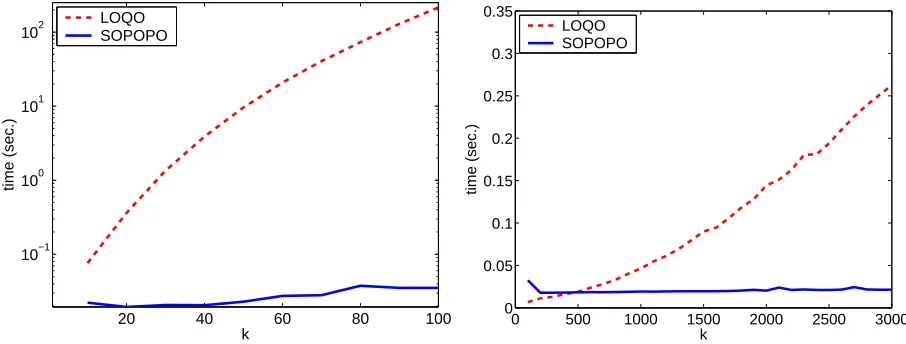
Our first set of experiments focuses on assessing the efficiency of SOPOPO for soft-projection onto a single polyhedron. In this set of experiments, the data was generated as follows. First, we chose the number of classes k=|Y|and defined E to be the set A×B with A= [k/2]and B= [k]\[k/2]. We set the value ofγrto be one for r∈A and otherwise it was set to zero. We then sampled an instance x and a set of vectors{u1, . . . ,uk}from a 100-dimensional Normal distribution of a zero mean and an identity matrix as a covariance matrix. After generating the instance and the targets, we presented the optimization problem of Eq. (7) to SOPOPO and to the LOQO optimization package. We repeated the above experiment for different values of k ranging from 10 through 100. For each value of k we repeated the entire experiment ten times, where in each trial we generated a new problem. We then averaged the results over the ten trials. The average CPU time consumed by the two algorithms as a function of k is depicted on the left hand side of Fig. 6. We would like to note that we have implemented SOPOPO both in Matlab and C++. We used the Matlab interface to LOQO, while LOQO itself was run in its native mode. We report results using our Matlab implementation of SOPOPO in order to eliminate possible implementation advantages. Our Matlab implementation follows the pseudo-code of Fig. 3. Nevertheless, as clearly indicated by the results, the time consumed by SOPOPO is negligible and exhibits only a very minor increase with k. In contrast, the run time of LOQO increases significantly with k. The apparent advantage of our algorithm over LOQO can be attributed to a few factors. First, LOQO is a general purpose

numerical optimization toolkit. Its generality is clearly a two edged sword as it employs a numerical

interior point method regardless of the problem on hand. Furthermore, LOQO was set to solve numerically the soft-projection problem of Eq. (7) while SOPOPO solves optimally the equivalent reduced problem of Eq. (19). To eliminate the latter mitigating factor which is in favor of SOPOPO, we repeated the same experiment as before while presenting to LOQO the reduced optimization problem rather than the original soft-projection problem. The results are depicted on the right hand side of Fig. 6. Yet again, the run time of SOPOPO is still significantly lower than LOQO for k>300 and as before there is no significant increase in the run time of SOPOPO as k increases.

sam-20 40 60 80 100 10−1

100 101 102

k

time (sec.)

LOQO SOPOPO

0 500 1000 1500 2000 2500 3000

0 0.05 0.1 0.15 0.2 0.25 0.3 0.35

k

time (sec.)

LOQO SOPOPO

Figure 6: A comparison of the run-time of SOPOPO and LOQO on the original soft-projection problem defined in Eq. (7) (left) and on the reduced problem from Eq. (19) (right).

pled a set of vectors {w1, . . . ,wk} from the same Gaussian distribution. For each instance xi, we calculated the vector vi∈Rk, whose r’th element is wr·xi. We then set Ai to be the indices of the top k/2 elements of vi while Bi consisted of all the rest of the elements,[k]\Ai. For example, assume that vi= (0.4,4.1,3.5,−2)then Ai={2,3}and Bi={1,4}. As feedback we setγi_a=1 for all a∈Ai and for b∈Biwe setγi_b=0. In our running example, the resulting vectorγi amounts to

(0,1,1,0). Finally, we set E(γi_{) ={E}i_{}, where E}i_{=A×B, and the value ofσwas always 1. We} repeated the above process for different values of k ranging from 20 through 100. The number of examples was fixed to be 10k and thus ranged from 200 through 1000. The value of C was set to be 1/m. In each experiment we terminated the wrapper procedure described in Fig. 5 when the gap

between the primal and dual objective functions went below 0.01. We first tried to execute LOQO with the original optimization problem described in Eq. (6). However, the resulting optimization problem was too large for LOQO to manage in a reasonable time, even for the smallest problem (k=20). Our iterative algorithm solves such small problems in less than a second. To facilitate a more meaningful comparison, we used the techniques described in Sec. 3 and replaced the original optimization problem from Eq. (6) with the following reduced problem,

max

α,β −

1 2

k

∑

r=1

_i:r

∑

_∈Ai

αi

rxi −

∑

i:r∈Bi

βi rxi

2

+

k

∑

r=1 i:r

∑

∈Ai

αi

rγir−

∑

i:r∈Bi

βi rγir

!

s.t. ∀i∈[m]:∀a∈Ai, αi_a≥0 and ∀b∈Bi, βi_b≥0

∀i∈[m]:

∑

a∈Ai

αi

a =

∑

b∈Bi

βi

b ≤ C .

(38)

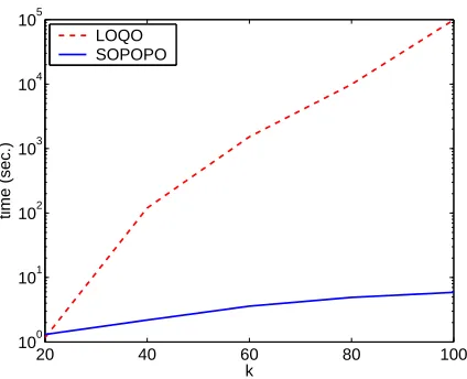
20 40 60 80 100 100

101 102 103 104 105

k

time (sec.)

LOQO SOPOPO

Figure 7: A comparison of the run-time in batch settings of SOPOPO and LOQO (using the reduced problem in Eq. (38)). The number of examples was set to be 10 times the number of labels (denoted k) in each problem.

value of k as the number of graphs grows with k. Nonetheless, even for k=100 the run time of SOPOPO’s wrapper does not exceed 4 seconds. These promising results emphasize the viability of our approach for large scale optimization problems.

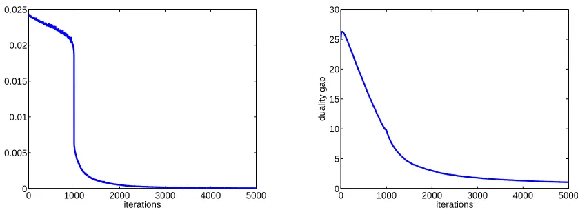
The last experiment underscores an interesting property of our iterative algorithm. In this ex-periment we have used the same data as in the previous exex-periment with k=100 and m=1000. After each iteration of the algorithm, we examined both the increase in the dual objective after the update and the difference between the primal and dual values. The results are shown in Fig. 8. The graphs exhibit a phenomena reminiscent of a phase transition. After about 1000 iterations, which is also the number of examples, the increase in the dual objective becomes miniscule. This phase transition is also exhibited for other choices of m, k and C. Note in addition that as the number of epochs increases, the increase of the dual objective becomes very small relatively to the duality gap. It is common to use the increase of the dual objective as a stopping criterion and the last experiment indicates that this criterion does not necessarily imply convergence. We leave further investigation of these phenomena to future research.