Infinitely Imbalanced Logistic Regression
Art B. Owen [email protected]
Department of Statistics Stanford University Stanford CA, 94305, USA
Editor: Yi Lin
Abstract
In binary classification problems it is common for the two classes to be imbalanced: one case is very rare compared to the other. In this paper we consider the infinitely imbalanced case where one class has a finite sample size and the other class’s sample size grows without bound. For logistic regression, the infinitely imbalanced case often has a useful solution. Under mild conditions, the intercept diverges as expected, but the rest of the coefficient vector approaches a non trivial and useful limit. That limit can be expressed in terms of exponential tilting and is the minimum of a convex objective function. The limiting form of logistic regression suggests a computational shortcut for fraud detection problems.
Keywords: classification, drug discovery, fraud detection, rare events, unbalanced data
1. Introduction
In many applications of logistic regression one of the two classes is extremely rare. In political science, the occurrence of wars, coups, vetos and the decisions of citizens to run for office have been modelled as rare events; see King and Zeng (2001). Bolton and Hand (2002) consider fraud detection, and Zhu et al. (2005) look at drug discovery. In other examples the rare event might correspond to people with a rare disease, customer conversions at an e-commerce web site, or false positives among a set of emails marked as spam.
We will let Y ∈ {0,1}denote a random response with the observed value of Y being y=1 in the rare case and y=0 in the common case. We will suppose that the number of observations with
y=0 is so large that we have a satisfactory representation of the distribution of predictors in that setting. Then we explore the limit as the number of y=0 cases tends to infinity while the number of observed cases with y=1 remains fixed. It is no surprise that the intercept term in the logistic regression typically tends to−∞in this limit. The other coefficients can however tend to a useful limit.
The main result (Theorem 8 below) is that under reasonable conditions, the intercept term tends to −∞ like −log(N) plus a constant, while the limiting logistic regression coefficient β=β(N) satisfies
¯
x=
R
ex0βx dF0(x) R
ex0β
dF0(x)
where F0is the distribution of X given Y =0 and ¯x is the average of the sample xivalues for which
y=1. The limiting solution is the exponential tilt required to bring the population mean of X given
Y =0 onto the sample mean of X given Y =1.
When F0is the N(µ0,Σ0)distribution for finite nonsingularΣ0then lim
N→∞β(N) =Σ −1
0 (x¯−µ0). (2)
Equation (2) reminds one of a well known derivation for logistic regression. If the conditional distribution of X given that Y =y is N(µy,Σ) then the coefficient of X in logistic regression is Σ−1(µ
1−µ0). Equation (2) however holds without assuming that the covariance of X is the same for Y =0 and Y =1, or even that X is Gaussian given that Y =1.
The outline of the paper is as follows. Section 2 gives three numerical examples that illustrate the limiting behavior ofβ. One is a positive result in which we seeβapproaching the value computed from (2). The other two examples are negative results where (1) does not hold. Each negative case illustrates the failure of an assumption of Theorem 8. In one case there is no nontrivial estimate ofβ at any N>0 while in the otherβdiverges as N→∞. Section 3 formally introduces the notation of this paper. It outlines the results of Silvapulle (1981) who completely characterizes the conditions under which unique logistic regression estimates exist in the finite sample case. The infinite sample case differs importantly and requires further conditions. A stronger overlap condition is needed between the two X distributions. Also, the distribution of X given Y =0 must not have tails that are too heavy, an issue that cannot arise in finite samples fromRd. Section 4 proves the results in this paper. A surprising consequence of Equation (1) is that the x values when y=1 only appear through their average ¯x. Section 5 shows that for the drug discovery example of Zhu et al. (2005), we can
replace all data points with y=1 by a single one at (x,¯ 1) with minimal effect on the estimated coefficient, apart from the intercept term. Section 6 discusses how these results can be used in deciding which unlabelled data points to label, and it shows how the infinitely imbalanced setting may lead to computational savings.
We conclude this introduction by relating the present work to the literature on imbalanced data. The English word “unbalanced” seems to be more popular, at least on web pages, than is “imbal-anced”. But the latter term has been adopted for this special setting in two recent workshops: AAAI 2000 and ICML 2003, respectively Japkowicz (2000) and Chawla et al. (2003). An extensive survey of the area is given by Chawla et al. (2004). In that literature much attention is paid to undersam-pling methods in which some of the available cases with Y =0 are either randomly or strategically removed to alleviate the imbalance. Another approach is oversampling in which additional, possibly synthetic, cases are generated with Y =1. It is also clear that prediction accuracy will be very good for a trivial method that always predicts y=0 and so one needs to take care about misclassification cost ratios and prior probability ratios.
2. Numerical Examples
N α Neα β
10 −3.19 0.4126 1.5746 100 −5.15 0.5787 1.0706 1,000 −7.42 0.6019 1.0108 10,000 −9.71 0.6058 1.0017 100,000 −12.01 0.6064 1.0003
Table 1: Logistic regression interceptαand coefficientβfor imbalanced data described in the text. There are N observations with Y =0 and stratified X ∼N(0,1)and one observation with
Y =1 and X=1.
clearer. Some resulting values are shown in Table 1. From this table it seems clear that as N→∞, the intercept term is diverging like −log(N) while the coefficient of X is approaching the value 1 that we would get from Equation (2). Theorem 8 below shows that such is indeed the limiting behavior.
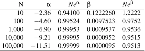
Next we repeat the computation replacingΦ by the CDF of the standard Cauchy distribution with density 1/(π(1+x2)). The results are shown in Table 2. Here it is clear thatβ→0 as N→∞ andαappears to behave like a constant minus log(N). It is not surprising thatβ→0 in this limit. The Cauchy distribution has tails far heavier than the logistic distribution. If β6=0 then the log likelihood (4) that we introduce in Section 3 is −∞. The likelihood is maximized at β=0 and
α=−log(N+1). We get slightly different values in Table 2 because the uniform distribution over
N Cauchy quantiles that we use has lighter tails than the actual Cauchy distribution it approaches.
The heavy tails of the Cauchy distribution make it fail a condition of Theorem 8. The finite sample setting does not need a tail condition on the distribution of X , beyond an assumption that all observed values are finite.
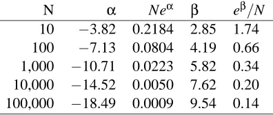
In the next example we use the U(0,1)distribution for X given Y =0. This time we use n=2 points with y=1. One has x=1/2 and the other has x=2. The results are shown in Table 3. Once again the valueβdoes not appear to be converging to a limit. It cannot be due to heavy tails, because the U(0,1)distribution has bounded support. On further thought, we see that ¯x=5/4. There is no possible way for an exponential tilt like (1) to reweight the U(0,1)distribution to have mean 5/4. This example also fails one of the conditions of Theorem 8. We need the point ¯x to be surrounded
by the distribution of X given Y =0 as defined in Section 3. Such a requirement is stronger than
N α Neα β Neβ
10 −2.36 0.94100 0.1222260 1.2222 100 −4.60 0.99524 0.0097523 0.9752 1,000 −6.90 0.99953 0.0009537 0.9536 10,000 −9.21 0.99995 0.0000952 0.9515 100,000 −11.51 0.99999 0.0000095 0.9513
N α Neα β eβ/N
10 −3.82 0.2184 2.85 1.74 100 −7.13 0.0804 4.19 0.66 1,000 −10.71 0.0223 5.82 0.34 10,000 −14.52 0.0050 7.62 0.20 100,000 −18.49 0.0009 9.54 0.14
Table 3: Logistic regression interceptαand coefficientβfor imbalanced data described in the text. There are N observations with Y =0 and stratified X∼U(0,1)and two observations with
Y =1, one with X =1/2, the other with X =2.
what is needed in the finite sample setting. Empirically eα and eβboth appear to follow a power law in N but we do not investigate this further, focusing instead on the case whereβapproaches a non-trivial limit.
3. Notation
The data are(x,y)pairs where x∈Rd and y∈ {0,1}. There are n observations with y=1 and N with y=0. The difference in case serves to remind us that nN. The values of x when y=1 are
x11, . . . ,x1n. The values of x when y=0 are x01, . . . ,x0N. Singly subscripted values xirepresent x1i.
Sometimes we use n1for n and n0for N.
The logistic regression model is Pr(Y=1|X=x) =eα+x0β/(1+eα+x0β)forα∈Randβ∈Rd. The log-likelihood in logistic regression is
n
∑
i=1 n
α+x01iβ−log(1+eα+x01iβ)
o −
N
∑
i=1
log(1+eα+x0i0β). (3)
We suppose that a good approximation can be found for the conditional distribution of X given that Y =0, as seems reasonable when N is very large. For continuously distributed X we might then replace the second sum in (3) by NR
log(1+exp(1+eα+x0β)f0(x)dx where f0is a probability density function. Because some or all of the components of X might be discrete we work instead with a distribution function F0for X given that Y =0.
With a bit of foresight we also center the logistic regression around the average ¯x=∑n
i=1xi/n of the predictor values for cases with Y=1. Then the log likelihood we work with simplifies to
`(α,β) =nα−
n
∑
i=1
log(1+eα+(xi−x¯)0β)−N
Z
log(1+eα+(x−x¯)0β)dF0(x) (4) where the nαterm arises as∑ni=1α+ (xi−x¯)0β.
When the centered log likelihood`has an MLE(αˆ0,βˆ)we can recover the MLE of the uncen-tered log likelihood easily: ˆβremains unchanged while ˆαin the uncentered version is ˆα0−x¯0βˆ. The numerical examples in Section 2 used uncentered logistic regression.
Here we study the maximizer(α,ˆ βˆ)of (4) in the limit as N→∞with n and x1, . . . ,xnheld fixed.
It is reasonable to suppose that ˆα→ −∞in this limit. Indeed we anticipate eαˆ should be O(1/N) since the proportion of observations with y=1 in the data is n/(N+n)=. n/N. What is interesting
3.1 Silvapulle’s Results
It is well known that the MLE in the usual logistic regression setting can fail to be finite when the x values where y=1 are linearly separable from those where y=0.
The existence and uniqueness of MLE’s for linear logistic regression has been completely char-acterized by Silvapulle (1981). He works in terms of binary regression through the origin. To employ an intercept, one uses the usual device of adjoining a predictor component that is always equal to 1.
For y=1 let z1i= (1,x01i)0for i=1, . . . ,n1and for y=0 let z0i= (1,x00i)0 for i=1, . . . ,n0. Let
θ= (α,β0)0. Then the logistic regression model has Pr(Y =1|X =x) =exp(z0θ)/(1+exp(z0θ)) where of course z=z(x) = (1,x0)0. Silvapulle (1981) employs two convex cones:
Cj=
(n
j
∑
i=1
kjizji|kji>0
)
, j∈ {0,1}.
Theorem 1 For data as described above, assume that the n0+n1by d+1 matrix with rows taken
from zji for j=0,1 and i=1, . . . ,nj has rank d+1. If C0∩C16= /0 then a unique finite logistic
regression MLE ˆθ= (α,ˆ βˆ0)exists. If however C0∩C1=/0then no MLE exists.
Proof: This result follows from clause (iii) of the Theorem on page 311 of Silvapulle (1981).
Silvapulle (1981) has more general results. Theorem 1 also holds when the logistic CDF G(t) = exp(t)/(1+exp(t))is replaced by the standard normal one (for probit analysis) or by the U(0,1) CDF. Any CDF G for which both−log G(t)and−log(1−G(t))are convex, and for which G(t)is strictly increasing when 0<G(t)<1 obeys the same theorem. The CDF G cannot be the Cauchy CDF, because the Cauchy CDF fails the convexity conditions.
The cone intersections may seem unnatural. A more readily interpretable condition is that the relative interior (as explained below) of the convex hull of the x’s for y=0 intersects that for y=1. That is H0∩H16= /0where
Hj= (n
j
∑
i=1
λjixji|λji>0, nj
∑
i=1
λji=1 )
.
When the xji span Rd then Hj is the interior of the convex hull of xji. When xji lie in a lower
dimensional affine subspace ofRdthen the interior of their convex hull is the empty set. However the interior with respect to that subspace, called the relative interior, and denoted Hj above is not
empty. In the extreme where xji =xj1 for i=1, . . . ,nj, then the desired relative interior of the
convex hull of xj1, . . . ,xjnj is simply{xj1}.
Lemma 2 In the notation above H0∩H16=/0if and only if C0∩C16=/0.
Proof: Suppose that x0∈H0∩H1. Then z0 = (1,x00)0 ∈C0∩C1. Conversely suppose that z0∈
C0∩C1. Then we may write
z0=
n0
∑
i=1
k0i
1
x0i
=
n1
∑
i=1
k1i
1
x1i
,
3.2 Overlap Conditions
In light of Silvapulle’s results we expect that we will need to assume some overlap between the data
x1, . . . ,xnfrom the 1s and the distribution F0of X given Y =0 in order to get a nontrivial result. The setting here with N→∞is different and requires a stronger, but still very weak, overlap condition. In describing this condition, we letΩ={ω∈Rd|ω0ω=1}be the unit sphere inRd.
Definition 3 The distribution F onRd has the point x∗surrounded if
Z
(x−x∗)0ω>ε
dF(x)>δ (5)
holds for someε>0, someδ>0 and allω∈Ω.
We will make use of two simple immediate consequences of (5). If F has the point x∗ sur-rounded, then there existηandγsatisfying
inf
ω∈Ω
Z
(x−x∗)0ω≥0dF(x)≥η>0 (6) and
inf
ω∈Ω
Z
[(x−x∗)0ω]+dF(x)≥γ>0 (7)
where Z+=max(Z,0)is the positive part of Z. For example we can takeη=δin (6) andγ=εδ in (7). Notice that F cannot surround any point if F concentrates in a low dimensional affine subset ofRd. This implies that having at least one point surrounded by F0 will be enough to avoid rank deficiency.
In Theorem 1 it follows from Lemma 2 that we only need there to be some point x∗ that is surrounded by both ˆF0and ˆF1where ˆFjis the empirical distribution of xj1, . . . ,xjnj. If such x exists,
we get a unique finite MLE. (Recall that Theorem 1 assumes full rank for the predictors.)
In the infinitely imbalanced setting we expect that F0will ordinarily surround every single one of x1, . . . ,xn. We do not need F0to surround them all but it is not enough to just have some point x∗ exist that is surrounded by both F0and ˆF1. We need to assume that F0surrounds ¯x. We do not need to assume that ˆF1surrounds ¯x, a condition that fails when the xi are confined to an affine subset of
Rdas they necessarily are for n<d.
There is an interesting case in which F0 can fail to surround ¯x. The predictor X may contain
a component that is itself an imbalanced binary variable, and that component might never take the value 1 in the y=1 sample. Then ¯x is right on the boundary of the support of F0and we cannot be sure of a finiteβin either the finite sample case or the infinitely imbalanced case.
3.3 Technical Lemmas
The first technical lemma below is used to get some bounds. The second one establishes existence of a finite MLE when N<∞.
Lemma 4 Forα,z∈R,
eα+z≥log(1+eα+z)≥[log(1+eα) +zeα/(1+eα)]+ ≥[zeα/(1+eα)]+=z+eα/(1+eα).
Proof: For the leftmost inequality, apply x≥log(1+x) to x=eα+z. For the others, the func-tion h(z) =log(1+eα+z)is convex and positive. Therefore h(z)≥[h(0) +zh0(0)]+≥[zh0(0)]+=
z+h0(0).
Lemma 5 Let n≥1 and x1, . . . ,xn∈Rd be given, and assume that the distribution F0 surrounds ¯
x=∑n
i=1xi/n and that 0<N<∞. Then the log likelihood`(α,β)given by (4) has a unique finite maximizer(α,ˆ βˆ).
Proof: The log likelihood`is strictly concave in(α,β). It either has a unique finite maximizer or it grows forever along some ray{(λα0,λβ0)|0≤λ<∞} ⊂Rd+1. By following such a ray back to where it intersects a small cylinder around the origin we may assume that either 0≤ |α0|<ε/2 and
β0
0β0=1, whereεis the constant in Definition 3, or that 0<|α0|<ε/2 andβ0=0. We will show that∂`(λα0,λβ0)/∂λis always strictly negative, ruling out infinite growth and thus establishing a unique finite maximizer.
For β0=0 andα0>0 we find limλ→∞∂`(λα0,λβ0)/∂λ=−Nα0<0.Forβ0=0 andα0<0 we find limλ→∞∂`(λα0,λβ0)/∂λ=nα0<0.
Now supposeβ00β0=1 and|α0|<ε/2. Using nα0=∑ni=1α0+ (xi−x¯)0β0, we find
lim
λ→∞
∂
∂λ`(λα0,λβ0) =
∑
i:α0+(xi−x¯)0β0<0
α0+ (xi−x¯)0β0
−N
Z
α0+(x−x¯)0β0>0
α0+ (x−x¯)0β0dF0(x).
(9)
The sum in (9) is either 0 or is negative and the integral is either 0 or is positive. For the integral to be 0 we must have(x−x¯)0β0≤ −α0with probability one for x∼F0. But this is impossible because
F0has ¯x surrounded.
4. Main Results
Lemma 6 below shows that, as anticipated, eαˆ is typically O(1/N)as N→∞. Specifically, we find a bound B=2n/η<∞for which lim supN→∞Neαˆ <B.
Lemma 6 Under the conditions of Lemma 5, let ˆαand ˆβmaximize`of (4). Letηsatisfy (6). Then for N≥2n/ηwe have eαˆ ≤2n/(Nη).
Proof: Letβbe any point inRd. Write eα=A/N for 0<A<∞. Then
∂
∂α`=n− n
∑
i=1
AN−1e(xi−¯x)0β
1+AN−1e(xi−x¯)0β−N
Z AN−1e(x−x¯)0β
1+AN−1e(x−x¯)0βdF0(x) ≤n−A
Z
(x−¯x)0β≥0
e(x−x¯)0β
1+AN−1e(x−x¯)0βdF0(x) ≤n− Aη
Now suppose that N≥2n/ηand that eα>2n/(Nη), that is A>2n/η. Then∂`/∂α<0. Because
`is concave this negative partial derivative implies that
arg max
α `(α,β)<log(2n/η)−log(N). (10)
Because βwas arbitrary (10) holds for allβ∈Rd. Lemma 5 implies that ˆβis finite, and so (10) applies forβ=βˆ.
Lemma 7 Under the conditions of Lemma 5, let ˆαand ˆβmaximize`of (4). Then lim supN→∞kβˆk< ∞.
Proof: Let eα=A/N for A>0 and letβ∈Rd. Pickγto satisfy (7). Then
`(α,0)−`(α,β)
=−(n+N)log(1+eα) +
n
∑
i=1
log(1+eα+(xi−¯x)0β)
+N
Z
log(1+eα+(x−x¯)0β)dF0(x)
>−(n+N)eα+N e
α
1+eα
Z
(x−x¯)0β≥0(x−x¯) 0βdF
0(x) ≥ −(n+N)A
N+A
kβkγ 1+A/N
after applying two inequalities from (8) and making some simplifications. If follows that`(α,β)< `(α,0) wheneverkβk ≥γ−1(1+A/N)(1+n/N). For large enough N we havekβˆk ≤2/γ, using Lemma 6 to control A.
As illustrated in Section 2, infinitely imbalanced logistic regression will be degenerate if F0has tails that are too heavy. We assume that
Z
ex0β(1+kxk)dF0(x)<∞, ∀β∈Rd. (11)
Condition (11) is satisfied by distributions with bounded support and by light tailed distributions such as the multivariate normal distribution.
Theorem 8 Let n≥1 and x1, . . . ,xn∈Rd be fixed and suppose that F0 satisfies the tail
condi-tion (11) and surrounds ¯x=∑n
i=1xi/n as described at (5). Then the maximizer (α,ˆ βˆ) of` given by (4) satisfies
lim
N→∞ R
ex0βˆx dF0(x) R
ex0βˆ
dF0(x) =x.¯
Proof: Setting∂`/∂β=0, dividing by Neαˆ−x¯0βˆ and rearranging terms, gives Z (x−x¯)ex0βˆ
1+eαˆ+(x−x¯)0βˆdF0(x) =− 1
N n
∑
i=1
ex0iβˆ(xi−x¯)
1+eαˆ+(xi−x¯)0βˆ
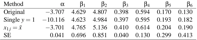
Method α β1 β2 β3 β4 β5 β6 Original −3.707 4.629 4.807 0.398 0.594 0.170 0.130 Single y=1 −10.116 4.623 4.984 0.397 0.595 0.193 0.182
x1 j=x¯ −3.701 4.765 5.136 0.410 0.614 0.204 0.190 SE 0.041 0.696 0.851 0.040 0.130 0.299 0.413
Table 4: This table shows logistic regression coefficients for the chemical compound data set de-scribed in the text. The top row shows ordinary logistic regression coefficients. The second row shows the coefficients when the cases with y=1 are deleted and replaced by a single point(x,¯ 1). The third row shows the coefficients when all 608 cases with y=1 are re-placed by(x,¯ 1). The fourth row shows standard errors for the ordinary logistic regression coefficients in the top row.
As N→∞the right side of (12) vanishes becausekβˆkis bounded as N→∞by Lemma 7. Therefore the MLEs satisfy
lim
N→∞ R
x ex0βˆ[1+eαˆ+(x−¯x)0βˆ]−1dF 0(x) R
ex0βˆ
[1+eαˆ+(x−x¯)0βˆ ]−1dF
0(x)
=x.¯ (13)
The denominator of (13) is at mostR
ex0βˆdF0(x)and is at least Z
ex0βˆ(1−eαˆ+(x−x¯)0βˆ)dF0(x)→ Z
ex0βˆdF0(x)
as N→∞becauseα→ −∞andR
e2x0βˆdF0(x)<∞by the tail condition (11). Therefore the denom-inator of (13) has the same limit asR
ex0βˆdF0(x)as N→∞. Similarly the numerator has the same limit asR
ex0βˆx dF0(x). The limit for the denominator is finite and nonzero, and so the result follows.
5. Illustration
It is perhaps surprising that in the N→∞limit, the logistic regression depends on x1, . . . ,xn only through ¯x. The precise configuration of those n points inRd becomes unimportant. We could rotate them about ¯x, or replace each of them by ¯x, or even replace them by one single point at ¯x with Y =1 and still get the same ˆβin the N→∞limit.
To investigate whether this effect can hold in finite data sets, we look at an example from Zhu et al. (2005). They study a data set with 29,812 chemical compounds on which 6 predictor variables were measured. Compounds were rated as active (Y =1) or inactive (Y =0) and only 608 of the compounds were active.
Table 4 shows the logistic regression coefficients for this data, as well as what happens to them when we replace the 608 data points(x,y)with y=1 by a single point at(x,¯ 1), or by 608 points equal to(x,¯ 1). In a centered logistic regression the point(x,¯ 1)becomes(x¯−x,¯ 1) = (0, . . . ,0,1)∈
Rd+1.
to the original logistic regression than has the version with 608 points at(x,¯ 1). The differences inβ are quite small compared to the sampling uncertainty. We would reach the same conclusions about which predictors are most important in all three cases.
The linear predictor ˆα+βˆ0(x−x¯)was computed using the coefficients from each of these models (taking care to use the original xi’s not the versions set to ¯x.) The correlation between the linear
predictor from logistic regression to that fit with all xi=x is 0.¯ 999881. The correlation between the
linear predictor from logistic regression to that fit with just one(x,¯ 1) data point is still higher, at 0.999888. The two altered linear predictors have correlation 0.999998. Not surprisingly any two of these linear predictors plot as a virtual straight line. There will be no important differences in ROC curves, precision and recall curves or other performance measures among these three fits.
6. Discussion
This paper has focussed on establishing the limit of ˆβas N→∞. This section presents some context and motivation. Section 6.1 shows these findings lead to greater understanding of how logistic regression works or fails and how to improve it. Section 6.2 shows how even after passing to the limit the resulting model makes some useful predictions. Section 6.3 illustrates the special case of
F0that is Gaussian or a mixture of Gaussians. Section 6.4 describes how using infinitely imbalanced logistic regression may lead to cost savings in fraud detection settings.
6.1 Insight Into Logistic Regression
In the infinitely imbalanced limit, logistic regression only uses the y=1 data points through their average feature vector ¯x. This limiting behavior is a property of logistic regression, not of any
particular data set. It holds equally well in those problems for which logistic regression works badly as it does in problems where the Bayes rule is a logistic regression.
In the illustrative example we got almost the same logistic regression after replacing all the rare cases by a single point at ¯x. We would not expect this property for learning methods in general. For
example classification trees such as those fit by CART (Breiman et al., 1984) will ordinarily change a lot if all of the Y =1 cases are replaced by one or more points(x,¯ 1).
Logistic regression only has d parameters apart from the intercept, so it is clear that it cannot be as flexible as some other machine learning methods. But knowing that those parameters are very strongly tied to the d components of ¯x gives us insight into how logistic regression works on
imbalanced problems. It is reasonable to expect better results from logistic regression when the x1i are in a single tight cluster near ¯x than when there are outliers, or when the x1ipoints are in two well separated clusters in different directions from the bulk of F0.
The insight also suggests things to do. For example when we detect outliers among the x1i, shrinking them towards ¯x, or removing them should improve performance. When we detect sharp
clusters among x1ithen we might fit one logistic regression per cluster, separating that cluster from the x0i’s, and predict for new points by pooling the cluster specific results. Even an O(n2)clustering algorithm may be inexpensive in the Nn setting.
6.2 Nontrivial Limiting Predictions
In the infinitely imbalanced limit with N→∞we often find that ˆβconverges to a finite limit while ˆ
prediction purposes. But we are often interested in probability ratios with nontrivial limits such as:
Pr(Ye=1|X =ex) Pr(Y =1|X =x) →e
(ex−x)0β
.
For example if we are presented with a number of cases of potential fraud to investigate and have limited resources then we can rank them by x0βand investigate as many of the most likely ones as time or other costs allow.
Because this rank is derived from a probability ratio we can also take into account the monetary or other measured value of the cases. If the values of uncovering fraud in the two cases are v and e
v, respectively, then we might prefer to investigate the former when vex0β>veeex0β. If the costs of investigation are c andec then we might prefer the former when vex0β/c>eveex0β/ec.
In active learning problems one must choose which data to gather. There are several kinds of active learning, as described in Tong (2001). The interventional setting is very similar to statisti-cal experimental design. For example, Cohn et al. (1996) describe how to select training data for feedforward neural networks. In the selective setting, the investigator has a mix of labelled cases (both x and y known) and unlabelled cases (x known but y unknown), and must choose which of the unlabelled cases to get a label for. For example the label y might indicate whether a human expert says that a document with feature vector x is on a specific topic. In a rare event setting, finding the cases most likely to have y=1 is a reasonable proxy for finding the most informative cases, and one could then allocate a large part of the labelling budget to cases with high values of x0β.
6.3 Gaussian Mixtures F0
When F0is a nonsingular Gaussian distribution then as remarked in the introduction,β→Σ−10 (x¯−
µ0). The effective sample size of an imbalanced data set is often considered to be simply the number of rare outcomes. The formula forβdepends on the data only through ¯x, which as an average of n
observations clearly has effective sample size of n. In the limit where N→∞first and then n→∞ we getβ→Σ−10 (µ1−µ0)where µj=E(X|Y =j). A confidence ellipsoid for µ1translates directly into one forβ.
Gaussian mixture models are a flexible and widely used method for approximating distributions. They have the further advantage for the present problem that exponential tilts of Gaussian mixtures are also Gaussian mixtures. The result is a convenient expression to be solved forβ.
Suppose that
F0=
K
∑
k=1
λkN(µk,Σk)
whereλk>0 and∑Kk=1λk=1. If at least one of theΣkhas full rank then F0will surround the point ¯
x. Then the limitingβis defined through
¯
x= ∑
K
k=1λk(µk+Σkβ)eβ
0µ
k+β0Σkβ/2
∑K k=1λkeβ
0µ
k+β0Σkβ/2 ,
so thatβis the solution to
0=
K
∑
k=1
λk(µk+Σkβ−x¯)eβ
0µ
k+β0Σkβ/2. (14)
6.4 Computational Costs
The exponential tilting solution to (1) is the valueβfor whichR
(x−x¯)ex0βdF0(x) =0. That solution is more conveniently expressed as the root of
g(β)≡ Z
(x−x¯)e(x−x¯)0βdF0(x) =0. (15) Equation (15) is the gradient with respect toβof
f(β) =
Z
e(x−x¯)0βdF0(x), which has Hessian
H(β) =
Z
(x−x¯)(x−x¯)0e(x−x¯)0βdF0(x).
The tilting problem (1) can be solved by finding the root of (15) which is in turn equivalent to the minimization of the convex function f .
When F0is modeled as a mixture F0of Gaussians the objective function, gradient, and Hessian needed for optimization have a simple form. They are,
f(β) =
K
∑
k=1
λkeβ0(µ
k−x¯)+β0Σkβ/2,
g(β) =
K
∑
k=1
λk(eµk(β)−x¯)eβ
0(µ
k−x¯)+β0Σkβ/2, where,
eµk(β)≡µk+Σkβ, and,
H(β) =
K
∑
k=1
λkΣk+ (eµk(β)−x¯)(eµk(β)−x¯)0
eβ0(µk−x¯)+β0Σkβ/2.
The cost of solving (14) or (15) by an algorithm based on Newton’s method takes O(d3) com-putation per iteration. By contrast, each step in iteratively reweighted least squares fitting of logistic regression takes O((n+N)d2)work. Even if one downsamples the data set, perhaps keeping only
N=5n randomly chosen examples from the Y =0 cases, the work of an iteration is O(nd2). The one time cost to fit a mixture of Gaussians includes costs of order Nd2 to form covariance matrix estimates, or O(nd2)if one has downsampled. But after the first iteration there can be substantial computational savings for solving (15) instead of doing logistic regression, when n/d is large.
When there is one common class and there are numerous rare classes, such as types of fraud or different targets against which a drug might be active, then the cost of approximating F0can be shared over the set of uncommon classes.
Acknowledgments
This work was supported by NSF grants DMS-0306612 and DMS-0604939. I thank Alan Agresti, Trevor Hastie for their comments. Thanks also to the JMLR reviewers for their speedy and helpful reviews. I am grateful for many insightful comments from Paul Louisell.
References
R. J. Bolton and D. J. Hand. Statistical fraud detection: A review. Statistical Science, 17(3):235– 255, 2002.
L. Breiman, J.H. Friedman, R.A. Olshen, and C.J. Stone. Classification And Regression Trees. Wadsworth, Belmont, CA, 1984.
N.V. Chawla, N. Japkowicz, and A. Kolcz. Proceedings of the ICML’2003 Workshop on Learning
from Imbalanced Data Sets. 2003.
N.V. Chawla, N. Japkowicz, and A. Kolcz. Editorial: special issue on learning from imbalanced data sets. ACM SIGKDD Explorations Newsletter, 6(1):1–6, 2004.
D.A. Cohn, Z. Ghahramani, and M.I. Jordan. Active learning with statistical models. Journal of
Artificial Intelligence Research, 4:129–145, 1996.
N. Japkowicz. Learning from Imbalanced Data Sets: Papers from the AAAI Workshop. AAAI, 2000. Technical Report WS-00-05.
G. King and L. Zeng. Logistic regression in rare events data. Political Analysis, 9(2):137–163, 2001.
M.J. Silvapulle. On the existence of maximum likelihood estimates for the binomial response mod-els. Journal of the Royal Statistical Society, Series B, 43:310–313, 1981.
S. Tong. Active learning: Theory and applications. PhD thesis, Stanford University, 2001. URL http://ai.stanford.edu/∼stong/research.html/tong thesis.pdf.