Exploring Strategies for Training Deep Neural Networks
Hugo Larochelle [email protected]
Yoshua Bengio [email protected]
J´erˆome Louradour [email protected]
Pascal Lamblin [email protected]
D´epartement d’informatique et de recherche op´erationnelle Universit´e de Montr´eal
2920, chemin de la Tour
Montr´eal, Qu´ebec, Canada, H3T 1J8
Editor: L´eon Bottou
Abstract
Deep multi-layer neural networks have many levels of non-linearities allowing them to compactly represent highly non-linear and highly-varying functions. However, until recently it was not clear how to train such deep networks, since gradient-based optimization starting from random initial-ization often appears to get stuck in poor solutions. Hinton et al. recently proposed a greedy layer-wise unsupervised learning procedure relying on the training algorithm of restricted Boltz-mann machines (RBM) to initialize the parameters of a deep belief network (DBN), a generative model with many layers of hidden causal variables. This was followed by the proposal of another greedy layer-wise procedure, relying on the usage of autoassociator networks. In the context of the above optimization problem, we study these algorithms empirically to better understand their success. Our experiments confirm the hypothesis that the greedy layer-wise unsupervised training strategy helps the optimization by initializing weights in a region near a good local minimum, but also implicitly acts as a sort of regularization that brings better generalization and encourages inter-nal distributed representations that are high-level abstractions of the input. We also present a series of experiments aimed at evaluating the link between the performance of deep neural networks and practical aspects of their topology, for example, demonstrating cases where the addition of more depth helps. Finally, we empirically explore simple variants of these training algorithms, such as the use of different RBM input unit distributions, a simple way of combining gradient estimators to improve performance, as well as on-line versions of those algorithms.
Keywords: artificial neural networks, deep belief networks, restricted Boltzmann machines,
au-toassociators, unsupervised learning
1. Introduction
Training deep multi-layered neural networks is known to be hard. The standard learning strategy— consisting of randomly initializing the weights of the network and applying gradient descent using backpropagation—is known empirically to find poor solutions for networks with 3 or more hidden layers. As this is a negative result, it has not been much reported in the machine learning literature. For that reason, artificial neural networks have been limited to one or two hidden layers.
el-ements and parameters required to represent some functions (Bengio and Le Cun, 2007; Bengio, 2007). Whereas it cannot be claimed that deep architectures are better than shallow ones on every problem (Salakhutdinov and Murray, 2008; Larochelle and Bengio, 2008), there has been evidence of a benefit when the task is complex enough, and there is enough data to capture that complexity (Larochelle et al., 2007). Hence finding better learning algorithms for such deep networks could be beneficial.
An approach that has been explored with some success in the past is based on constructively adding layers. Each layer in a multi-layer neural network can be seen as a representation of the input obtained through a learned transformation. What makes a good internal representation of the data? We believe that it should disentangle the factors of variation that inherently explain the structure of the distribution. When such a representation is going to be used for unsupervised learning, we would like it to preserve information about the input while being easier to model than the input itself. When a representation is going to be used in a supervised prediction or classification task, we would like it to be such that there exists a “simple” (i.e., somehow easy to learn) mapping from the representation to a good prediction. To constructively build such a representation, it has been proposed to use a supervised criterion at each stage (Fahlman and Lebiere, 1990; Lengell ´e and Denoeux, 1996). However, as we discuss here, the use of a supervised criterion at each stage may be too greedy and does not yield as good generalization as using an unsupervised criterion. Aspects of the input may be ignored in a representation tuned to be immediately useful (with a linear classifier) but these aspects might turn out to be important when more layers are available. Combining unsupervised (e.g., learning about p(x)) and supervised components (e.g., learning about p(y|x)) can be be helpful when both functions p(x)and p(y|x)share some structure.
The idea of using unsupervised learning at each stage of a deep network was recently put for-ward by Hinton et al. (2006), as part of a training procedure for the deep belief network (DBN), a generative model with many layers of hidden stochastic variables. Upper layers of a DBN are supposed to represent more “abstract” concepts that explain the input observation x, whereas lower layers extract “low-level features” from x. In other words, this model first learns simple concepts, on which it builds more abstract concepts.
This training strategy has inspired a more general approach to help address the problem of train-ing deep networks. Hinton (2006) showed that stacktrain-ing restricted Boltzmann machines (RBMs)— that is, training upper RBMs on the distribution of activities computed by lower RBMs—provides a good initialization strategy for the weights of a deep artificial neural network. This approach can be extended to non-linear autoencoders or autoassociators (Saund, 1989), as shown by Bengio et al. (2007), and is found in stacked autoassociators network (Larochelle et al., 2007), and in the deep convolutional neural network (Ranzato et al., 2007b) derived from the convolutional neural network (LeCun et al., 1998). Since then, deep networks have been applied with success not only in clas-sification tasks (Bengio et al., 2007; Ranzato et al., 2007b; Larochelle et al., 2007; Ranzato et al., 2008), but also in regression (Salakhutdinov and Hinton, 2008), dimensionality reduction (Hinton and Salakhutdinov, 2006; Salakhutdinov and Hinton, 2007b), modeling textures (Osindero and Hin-ton, 2008), information retrieval (Salakhutdinov and HinHin-ton, 2007a), robotics (Hadsell et al., 2008), natural language processing (Collobert and Weston, 2008; Weston et al., 2008), and collaborative filtering (Salakhutdinov et al., 2007).
In this paper, we discuss in detail three principles for training deep neural networks and present experimental evidence that highlight the role of each in successfully training deep networks:
2. using unsupervised learning at each layer in a way that preserves information from the input and disentangles factors of variation;
3. fine-tuning the whole network with respect to the ultimate criterion of interest.
The experiments reported here suggest that this strategy improves on the traditional random initialization of supervised multi-layer networks by providing “hints” to each intermediate layer about the kinds of representations that it should learn, and thus initializing the supervised fine-tuning optimization in a region of parameter space from which a better local minimum (or plateau) can be reached. We also present a series of experiments aimed at evaluating the link between the performance of deep neural networks and aspects of their topology such as depth and the size of the layers. In particular, we demonstrate cases where the addition of depth helps classification error, but too much depth hurts. Finally, we explore simple variants of the aforementioned training algorithms, such as a simple way of combining them to improve their performance, RBM variants for continuous-valued inputs, as well as on-line versions of those algorithms.
2. Notations and Conventions
Before describing the learning algorithms that we will study and experiment with in this paper, we first present the mathematical notation we will use for deep networks.
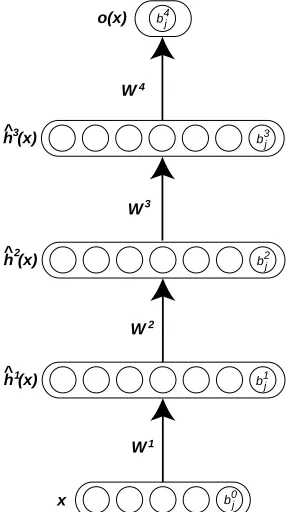
A deep neural network contains an input layer and an output layer, separated by l layers of hidden units. Given an input sample clamped to the input layer, the other units of the network compute their values according to the activity of the units that they are connected to in the layers below. We will consider a particular sort of topology here, where the input layer is fully connected to the first hidden layer, which is fully connected to the second layer and so on up to the output layer.
Given an input x, the value of the j-th unit in the i-th layer is denotedbhij(x), with i=0 referring to the input layer, i=l+1 referring to the output layer (the use of “b” will become clearer in Section 4). We refer to the size of a layer as|bhi(x)|. The default activation level is determined by the internal bias bijof that unit. The set of weights Wjki betweenbhik−1(x)in layer i−1 and unitbhij(x)
in layer i determines the activation of unitbhij(x)as follows:
bhij(x) =sigm aij where aij(x) =bij+
∑
k
Wjkibhik−1(x)∀i∈ {1, . . . ,l},withbh0(x) =x (1)
where sigm(·)is the sigmoid squashing function: sigm(a) = 1
1+e−a (alternatively, the sigmoid could be replaced by the hyperbolic tangent). Given the last hidden layer, the output layer is computed similarly by
o(x) =bhl+1(x) = f
al+1(x) where al+1(x) =bl+1+Wl+1bhl(x)
where the activation function f(·)depends on the (supervised) task the network must achieve. Typ-ically, it will be the identity function for a regression problem and the softmax function
fj(a) =softmaxj(a) =
eaj
∑K k=1eak
(2)
o(x)
W4
h (x)3
b3j
x h (x) h (x)
1 2
W
W W
1 2 3
b1j
b2j
b0j
b4j
^
^
^
Figure 1: Illustration of a deep network and its parameters.
When an input sample x is presented to the network, the application of Equation 1 at each layer will generate a pattern of activity in the different layers of the neural network. Intuitively, we would like the activity of the first layer neurons to correspond to low-level features of the input (e.g., edge orientations for natural images) and to higher level abstractions (e.g., detection of geometrical shapes) in the last hidden layers.
3. Deep Neural Networks
compactly (with fewer parameters) through the composition of many non-linearities, that is, with a deep architecture. When the representation of a concept requires an exponential number of elements (more generally exponential capacity), for example, with a shallow circuit, the number of training examples required to learn the concept may also be impractical. Smoothing the learned function by regularization would not solve the problem here because in these cases the target function itself is complicated and requires exponential capacity just to be represented.
3.1 Difficulty of Training Deep Architectures
Given a particular task, a natural way to train a deep network is to frame it as an optimization problem by specifying a supervised cost function on the output layer with respect to the desired target and use a gradient-based optimization algorithm in order to adjust the weights and biases of the network so that its output has low cost on samples in the training set. Unfortunately, deep networks trained in that manner have generally been found to perform worse than neural networks with one or two hidden layers.
We discuss two hypotheses that may explain this difficulty. The first one is that gradient descent can easily get stuck in poor local minima (Auer et al., 1996) or plateaus of the non-convex training criterion. The number and quality of these local minima and plateaus (Fukumizu and Amari, 2000) clearly also influence the chances for random initialization to be in the basin of attraction (via gradient descent) of a poor solution. It may be that with more layers, the number or the width of such poor basins increases. To reduce the difficulty, it has been suggested to train a neural network in a constructive manner in order to divide the hard optimization problem into several greedy but simpler ones, either by adding one neuron (e.g., see Fahlman and Lebiere, 1990) or one layer (e.g., see Lengell´e and Denoeux, 1996) at a time. These two approaches have demonstrated to be very effective for learning particularly complex functions, such as a very non-linear classification problem in 2 dimensions. However, these are exceptionally hard problems, and for learning tasks usually found in practice, this approach commonly overfits.
This observation leads to a second hypothesis. For high capacity and highly flexible deep net-works, there actually exists many basins of attraction in its parameter space (i.e., yielding different solutions with gradient descent) that can give low training error but that can have very different gen-eralization errors. So even when gradient descent is able to find a (possibly local) good minimum in terms of training error, there are no guarantees that the associated parameter configuration will provide good generalization. Of course, model selection (e.g., by cross-validation) will partly cor-rect this issue, but if the number of good generalization configurations is very small in comparison to good training configurations, as seems to be the case in practice, then it is likely that the training procedure will not find any of them. But, as we will see in this paper, it appears that the type of unsupervised initialization discussed here can help to select basins of attraction (for the supervised fine-tuning optimization phase) from which learning good solutions is easier both from the point of view of the training set and of a test set.
3.2 Unsupervised Learning as a Promising Paradigm for Greedy Layer-Wise Training
A common approach to improve the generalization performance of a learning algorithm which is motivated by the Occam’s razor principle is the use of regularization (such as weight decay) that will favor “simpler” models over more complicated ones. However, using generic priors such as the
learn-ing task should be. This has motivated researchers to discover more meanlearn-ingful, data-dependent regularization procedures, which are usually based on unsupervised learning and normally adapted to specific models.
For example, Ando and Zhang (2005) use “auxiliary tasks” designed from unlabelled data and that are appropriate for a particular learning problem, to learn a better regularization term for linear classifiers. Partial least squares (Frank and Friedman, 1993) can also be seen as combining unsuper-vised and superunsuper-vised learning in order to learn a better linear regression model when few training data are available or when the input space is very high dimensional.
Many semi-supervised learning algorithms also involve a combination of unsupervised and su-pervised learning, where the unsusu-pervised component can be applied to additional unlabelled data. This is the case for Fisher-kernels (Jaakkola and Haussler, 1999) which are based on a generative model trained on unlabelled input data and that can be used to solve a supervised problem defined for that input space. In all these cases, unsupervised learning can be seen as adding more constraints on acceptable configurations for the parameters of a model, by asking that it not only describes well the relationship between the input and the target but also contains relevant statistical information about the structure of the input or how it was generated.
Moreover, there is a growing literature on the distinct advantages of generative and discrimi-native learning. Ng and Jordan (2001) argue that generative versions of discrimidiscrimi-native models can be expected to reach their usually higher asymptotic out-of-sample classification error faster (i.e., with less training data), making them preferable in certain situations. Moreover, successful attempts at exploring the space between discriminative and generative learning have been studied (Lasserre et al., 2006; Jebara, 2003; Bouchard and Triggs, 2004; Holub and Perona, 2005).
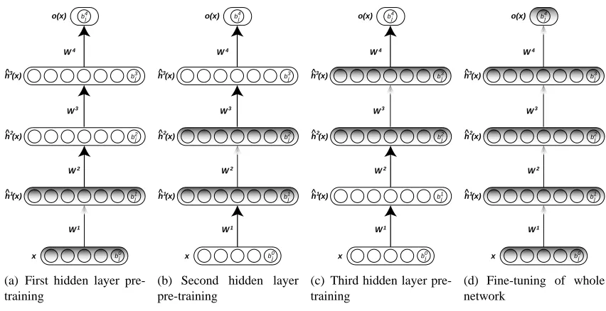
The deep network learning algorithms that have been proposed recently and that we study in this paper can be seen as combining the ideas of greedily learning the network to break down the learning problem into easier steps, using unsupervised learning to provide an effective hint about what hidden units should learn, bringing along the way a form of regularization that prevents overfitting even in deep networks with many degrees of freedom (which could otherwise overfit). In addition, one should consider the supervised task the network has to solve. The greedy layer-wise unsupervised strategy provides an initialization procedure, after which the neural network is fine-tuned to the global supervised objective. The general paradigm followed by these algorithms (illustrated in Figure 2 and detailed in Appendix A) can be decomposed in two phases:
1. In the first phase, greedily train subsets of the parameters of the network using a layer-wise and unsupervised learning criterion, by repeating the following steps for each layer (i∈ {1, . . . ,l})
Until a stopping criteria is met, iterate through training database by
(a) mapping input training sample xt to representation bhi−1(xt)(if i>1) and hidden
representationbhi(xt),
(b) updating parameters bi−1, bi and Wi of layer i using some unsupervised learning
algorithm.
o(x)
W4
h (x)3
b3j
x h (x) h (x) 1 2 W W W 1 2 3 b1 j b2 j
b0j
b4j
^
^
^
(a) First hidden layer pre-training
o(x)
W4
h (x)3
b3j
x h (x) h (x) 1 2 W W W 1 2 3 b1 j b2 j
b0j
b4j
^
^
^
(b) Second hidden layer pre-training
o(x)
W4
h (x)3
b3j
x h (x) h (x) 1 2 W W W 1 2 3 b1 j b2 j
b0j
b4j
^
^
^
(c) Third hidden layer pre-training
o(x)
W4
h (x)3
b3j
x h (x) h (x) 1 2 W W W 1 2 3 b1 j b2 j
b0j
b4j
^
^
^
(d) Fine-tuning of whole network
Figure 2: Unsupervised greedy layer-wise training procedure.
2. In the second and final phase, fine-tune all the parametersθof the network using backpropa-gation and gradient descent on a global supervised cost function C(xt,yt,θ), with input xtand
label yt, that is, trying to make steps in the direction E
h∂C(x t,yt,θ)
∂θ
i .
Regularization is not explicit in this procedure, as it does not come from a weighted term that depends on the complexity of the network and that is added to the global supervised objective. Instead, it is implicit, as the first phase that initializes the parameters of the whole network will ultimately have an impact on the solution found in the second phase (the fine-tuning phase). Indeed, by using an iterative gradual optimization algorithm such as stochastic gradient descent with early-stopping (i.e., training until the error on a validation set reaches a clear minimum), the extent to which the configuration of the network’s parameters can be different from the initial configuration given by the first phase is limited. Hence, similarly to using a regularization term on the parameters of the model that constrains them to be close to a particular value (e.g., 0 for weight decay), the first phase here will ensure that the parameter solution for each layer found by fine-tuning will not be far from the solution found by the unsupervised learning algorithm. In addition, the non-convexity of the supervised training criterion means that the choice of initial parameter values can greatly influence the quality of the solution obtained by gradient descent.
In the next two sections, we present a review of the two training algorithms that fall in paradigm presented above and which are empirically studied in this paper, in Section 6.
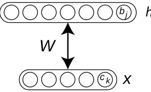
4. Stacked Restricted Boltzmann Machine Network
W
bj
ck
x
Figure 3: Illustration of a restricted Boltzmann machine and its parameters. W is a weight matrix, b is a vector of hidden unit biases, and c a vector of visible unit biases.
Figure 3 for an illustration), given an input x, it is easy to obtain a hidden representation for that input by computing the posteriorbh(x)over the layer of binary hidden variables h (we use the “b” symbol to emphasize thatbh(x)is not a random variable but a deterministic representation of x).
Hinton (2006) argues that this representation can be improved by giving it as input to another RBM, whose posterior over its hidden layer will then provide a more complex representation of the input. This process can be repeated an arbitrary number of times in order to obtain ever more non-linear representations of the input. Finally, the parameters of the RBMs that compute these rep-resentations can be used to initialize the parameters of a deep network, which can then be fine-tuned to a particular supervised task. This learning algorithm clearly falls in the paradigm of Section 3.2, where the unsupervised part of the learning algorithm is that of an RBM. We will refer to deep networks trained using this algorithm as stacked restricted Boltzmann machine (SRBM) networks. For more technical details about the SRBM network, and how to train an RBM using the contrastive divergence algorithm (CD-k), see Appendix B.
5. Stacked Autoassociators Network
There are theoretical results about the advantage of stacking many RBMs into a DBN: Hinton et al. (2006) show that this procedure optimizes a bound on the likelihood of the input data when all layers have the same size. An additional hypothesis to explain why this process provides a good initialization for the network is that it makes each hidden layer compute a different, possibly more abstract representation of the input. This is done implicitly, by asking that each layer captures fea-tures of the input that help characterize the distribution of values at the layer below. By transitivity, each layer contains some information about the input. However, stacking any unsupervised learning model does not guarantee that the representations learned get increasingly complex or appropriate as we stack more layers. For instance, many layers of linear PCA models could be summarized by only one layer. However, there may be other non-linear, unsupervised learning models that, when stacked, are able to improve the learned representation at the last layer added.
x
ck
bj x
W W* ^
h(x)^
Figure 4: Illustration of an autoassociator and its parameters. W is the matrix of encoder weights and W∗the matrix of decoder weights.bh(x)is the code or representation of x.
representation of x is a codebh(x)obtained from the encoding function
bhj(x) = f(aj) where aj(x) =bj+
∑
kWjkxk. (3)
The input’s reconstruction is obtained from a decoding function, here a linear transformation of the hidden representation with weight matrix W∗, possibly followed by a non-linear activation function:
b
xk=g(abk) whereabk=ck+
∑
jWjk∗bhj(x).
In this work, we used the sigmoid activation function for both f(·) and g(·). Figure 4 shows an illustration of this model.
By noticing the similarity between Equations 3 and 1, we are then able to use the training algorithm for autoassociators as the unsupervised learning algorithm for the greedy layer-wise ini-tialization phase of deep networks. In this paper, stacked autoassociators (SAA) networks will refer to deep networks trained using the procedure of Section 3.2 and the learning algorithm of an autoassociator for each layer, as described in Section 5.1.
Though these neural networks were designed with the goal of dimensionality reduction in mind, the new representation’s dimensionality does not necessarily need to be lower than the input’s in practice. However, in that particular case, some care must be taken so that the network does not learn a trivial identity function, that is, finds weights that simply “copy” the whole input vector in the hidden layer and then copy it again at the output. For example, a network with small weights Wjk
the case of binary inputs, if the weights are large, the input vector can still be copied (up to a permutation of the elements) to the hidden units, and in turn these used to perfectly reconstruct the input. Weight decay can be useful to prevent such a trivial and uninteresting mapping to be learned, when the inputs are binary. We set WT=W∗in all of our experiments. Vincent et al. (2008) have an improved way of training autoassociators in order to produce interesting, non-trivial features in the hidden layer, by partially corrupting the network’s inputs.
The reconstruction error of an autoassociator can be connected to the log-likelihood of an RBM in several ways. Ranzato et al. (2008) connect the log of the numerator of the input likelihood with a form of reconstruction error (where one replaces the sum over hidden unit configurations by a maximization). The denominator is the normalization constant summing over all input configura-tions the same expression as in the numerator. So whereas maximizing the numerator is similar to minimizing reconstruction error for the training examples, minimizing the denominator means that most input configurations should not be reconstructed well. This can be achieved if the autoassoci-ator is constrained in such a way that it cannot compute the identity function, but only minimizes the reconstruction for training examples.
Another connection between reconstruction error and log-likelihood of the RBM was made in Bengio and Delalleau (2007). They consider a converging series expansion of the log-likelihood gradient and show that whereas CD-k truncates the series by keeping the first 2k terms and then approximates expectations by a single sample, reconstruction error is a mean-field approximation of the first term in that series.
5.1 Learning in an Autoassociator Network
Training an autoassociator network is almost identical to training a standard artificial neural net-work. Given a cost function, backpropagation is used to compute gradients and perform gradient descent. However, autoassociators are “self-supervised”, meaning that the target to which the output of the autoassociator is compared is the input that it was fed.
Previous work on autoassociators minimized the squared reconstruction error:
C(bx,x) =
∑
k
(bxk−xk)2.
However, with squared reconstruction error and linear decoder, the “optimal codes” (the implicit target for the encoder, irrespective of the encoder) are in the span of the principal eigenvectors of the input covariance matrix. When we introduce a saturating non-linearity such as the sigmoid, and we want to reconstruct values[0,1], the binomial KL divergence (also known as cross-entropy) seems more appropriate:
C(bx,x) =−
∑
k(xklog(xbk) + (1−xk)log(1−bxk)). (4)
6. Experiments
In this section, we present several experiments set up to evaluate the deep network learning algo-rithms that fall in the paradigm presented in the Section 3.2 and highlight some of their properties. Unless otherwise stated, stochastic gradient descent was used for layer-wise unsupervised learning (first phase of the algorithm) and global supervised fine-tuning (second phase of the algorithm). The data sets were separated in disjoint training, validation and testing subsets. Model selection consisted of finding the best values for the learning rates of layer-wise unsupervised and global su-pervised learning as well as the number of unsusu-pervised updates preceding the fine-tuning phase. The number of epochs of fine-tuning was chosen using early-stopping based on the progression of classification error on the validation set. All experiments correspond to classification problems. Hence, to fine-tune the deep networks, we optimized the negative conditional log-likelihood of the training samples’ target class (as given by the softmax output of the neural network).
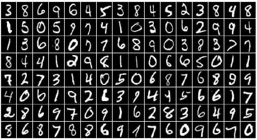
The experiments are based on the MNIST data set1(see Figure 5), a benchmark for handwritten digit recognition, as well as variants of this problem where the input distribution has been made more complex by inserting additional factors of variations, such as rotations and background images. The input images are made of 28×28 pixels giving an input dimensionality of 784, the number of classes is 10 (corresponding to the digits from 0 to 9) and the inputs were scaled between 0 and 1.
Successful applications of deep networks have already been presented on a large variety of data, such as images of faces (Salakhutdinov and Hinton, 2008), real-world objects (Ranzato et al., 2007a) as well as text data (Hinton and Salakhutdinov, 2006; Salakhutdinov and Hinton, 2007a; Collobert and Weston, 2008; Weston et al., 2008), and on different types of problems such as regres-sion (Salakhutdinov and Hinton, 2008), information retrieval (Salakhutdinov and Hinton, 2007a), robotics Hadsell et al. (2008), and collaborative filtering (Salakhutdinov et al., 2007).
In Bengio et al. (2007), we performed experiments on two regression data sets, with non-image continuous inputs (UCI Abalone, and a financial data set), demonstrating the use of unsupervised (or partially supervised) pre-training of deep networks on these tasks. In Larochelle et al. (2007), we studied the performance of several architectures on various data sets, including variations of MNIST (with rotations, random background, and image background), and discrimination tasks between wide and tall rectangles, and between convex and non-convex images. On these tasks, deep networks compared favorably to shallow architectures.
Our focus is hence not on demonstrating their usefulness on a wide range of tasks, but on ex-ploring their properties empirically. Such experimental work required several weeks of cumulative CPU time, which restricted the number of data sets we could explore. However, by concentrat-ing on the original MNIST data set and harder versions of it, we were able not only to confirm the good performance of deep networks, but also to study practical variations, to help understand the algorithms, and to discuss the impact on a deep network’s performance of stepping to a more complicated problem.
6.1 Validating the Unsupervised Layer-Wise Strategy for Deep Networks
In this section, we evaluate the advantages brought by the unsupervised layer-wise strategy of Sec-tion 3.2. We want to separate the different algorithmic concepts behind it, in order to understand their contribution to the whole strategy. In particular, we pursue the following two questions:
0 0.1 0.2 0.3 0.4 0.5 0.6 0.7 0.8 0.9 1 0
0.1 0.2 0.3 0.4 0.5 0.6 0.7 0.8 0.9 1
Figure 5: Samples from the MNIST digit recognition data set. Here, a black pixel corresponds to an input value of 0 and a white pixel corresponds to 1 (the inputs are scaled between 0 and 1).
1. To what extent does initializing greedily the parameters of the different layers help?
2. How important is unsupervised learning for this procedure?
To address these two questions, we will compare the learning algorithms for deep networks of Sections 4 and 5 with the following algorithms.
6.1.1 DEEPNETWORKWITHOUTPRE-TRAINING
To address the first question above, we compare the greedy layer-wise algorithm with a more stan-dard way to train neural networks: using stanstan-dard backpropagation and stochastic gradient descent, and starting at a randomly initialized configuration of the parameters. In other words, this variant simply puts away the pre-training phase of the other deep network learning algorithms.
6.1.2 DEEPNETWORKWITH SUPERVISEDPRE-TRAINING
To address the second question, we run an experiment with the following algorithm. We greedily pre-train the layers using a supervised criterion (instead of the unsupervised one), before performing as before a final supervised fine-tuning phase. Specifically, when greedily pre-training the param-eters Wi and bi, we also train another set of weights Vi and biases ci which connect hidden layer b
hi(x)to a temporary output layer as follows:
where f(·)is the softmax function of Equation 2. This output layer can be trained using the same cost as the global supervised cost. However, as this is a greedy procedure, only the parameters Wi, bi, Vi and ci are updated, that is, the gradient is not propagated to the layers below. When the training of a layer is finished, we can simply discard the parameters Vi and ci and move to pre-training the next hidden layer, having initialized Wiand bi.
6.1.3 STACKEDLOGISTIC AUTOREGRESSIONNETWORK
The second question aims at evaluating to what extent any unsupervised learning can help. We already know that stacking linear PCA models is not expected to help improve generalization. A slightly more complex yet very simple unsupervised model for data in[0,1]is the logistic autore-gression model (see also Frey, 1998)
b
xk=sigm bk+
∑
j6=kWk jxj
!
(5)
where the reconstruction bx is log-linear in the input x. The parameters W and b can be trained using the same cost used for the autoassociators in Equation 4. This model can be used to initialize the weights Wi and biases bi of the i-th hidden layer of a deep network. However, because W in Equation 5 is square, the deep network will need to have hidden layers with the same size as the input layer. Also, the weights on the diagonal of W are not trained in this model, so we initialize them to zero. The stacked logistic autoregression network will refer to deep networks using this unsupervised layer-wise learning algorithm.
6.1.4 RESULTS
The results for all these deep networks are given in Table 1. We also give results for a “shallow”, one hidden layer neural network, to validate the utility of deep architectures. Instead of the sigmoid, this network uses hyperbolic tangent squashing functions, which are usually found to work better for one hidden layer neural networks. The MNIST training set was separated into training (50,000) and validation (10,000) sets. The test set has size 10,000. In addition to the hyperparameters mentioned at the beginning of this section, the validation set was used also to select appropriate decrease constants2 for the learning rates of the greedy and fine-tuning phases. The SRBM and SAA networks had 500, 500 and 2000 hidden units in the first, second and third layers respectively, as in Hinton et al. (2006) and Hinton (2006). In the pre-training phase of the SRBM and SAA networks, when training the parameters of the i-th layer, the down-biases ckwhere set to be equal to
bik−1(although similar results were obtained by using a separate set of biases cik−1when the i−1-th layer is the down-layer). For the deep networks with supervised or no pre-training, different sizes of hidden layers were compared, including sizes similar to the stacked logistic autoregression network, and to the SRBM and SAA networks. All deep networks had 3 hidden layers.
Overall, the models that use the unsupervised layer-wise procedure of Section 3.2 outperform those that do not. We also observe a slight advantage in the performance of the SRBM network over that of the SAA network (on the MNIST test set, differences of more than 0.1% are statistically significant). The performance difference between the stacked logistic autoregressions network and
2. When using a decrease constantβ, the learning rate for the tthupdate becomes ε0
Models Train. Valid. Test SRBM (stacked restricted Boltzmann machines) network 0% 1.20% 1.20% SAA (stacked autoassociators) network 0% 1.31% 1.41% Stacked logistic autoregressions network 0% 1.65% 1.85% Deep network with supervised pre-training 0% 1.74% 2.04% Deep network, no pre-training 0.004% 2.07% 2.40% Shallow network, no pre-training 0% 1.91% 1.93%
Table 1: Classification error on MNIST training, validation, and test sets, with the best hyperpa-rameters according to validation error.
the deep network with supervised layer-wise pre-training particularly highlights the importance of unsupervised learning. Indeed, even though supervised layer-wise pre-training explicitly trains the hidden layers to capture non-linear information about the input, the overall procedure seems to be too greedy with respect to the supervised task to be learned. On the other hand, even though logistic autoregressions are simple log-linear models and their optimization is blind with respect to the future usage of the weights W as connections into non-linear hidden layers, the unsupervised nature of training makes them still useful for improving generalization. As a point of comparison, besides the deep networks, the best result on this data set reported for a learning algorithm that does not use any prior knowledge about the task (e.g., image pre-processing like deskewing or subsampling) is that of a support vector machine with a Gaussian kernel,3with 1.4% classification error on the test set.
At this point, it is clear that unsupervised layer-wise pre-training improves generalization. How-ever, we could wonder whether it also facilitates the optimization problem of the global fine-tuning. The results of Table 1 do not shed any light on this aspect. Indeed, all the networks, even those without greedy layer-wise pre-training, perform almost perfectly on the training set. The explana-tory hypothesis we evaluate here is that, without pre-training, the lower layers are initialized poorly, but still allow the top two layers to learn the training set almost perfectly because the output layer and the last hidden layer form a standard shallow but fat neural network. Consider the top two layers of the deep network with pre-training: it presumably takes as input a better representation, one that allows for better generalization. Instead, the network without pre-training sees a “random” transformation of the input, one that preserves enough information about the input to fit the training set, but that does not help to generalize. To test this hypothesis, we performed a second series of experiments in which we constrain the top hidden layer to be small (20 hidden units).
The results (Table 2) clearly suggest that optimization of the global supervised objective is made easier by greedy layer-wise pre-training. This result for supervised greedy pre-training is also coherent with past experiments on similar greedy strategies (Fahlman and Lebiere, 1990; Lengell ´e and Denoeux, 1996). Here, we have thus confirmed that it also applies to unsupervised greedy pre-training. With no pre-training, training error degrades significantly when there are only 20 hidden units in the top hidden layer. In addition, the results obtained without pre-training were found to have much larger variance than those with pre-training, indicating high sensitivity to initial
Models Train. Valid. Test
SRBM network 0% 1.5% 1.5%
SAA network 0% 1.38% 1.65%
Deep network with supervised pre-training 0% 1.77% 1.89% Deep network, no pre-training 0.59% 2.10% 2.20% Shallow network, no pre-training 3.6% 4.77% 5.00%
Table 2: Classification error on MNIST training, validation, and test sets, with the best hyperpa-rameters according to validation error, when the last hidden layer only contains 20 hidden units
conditions: the unsupervised pre-training more consistently puts the parameters in a “good” basin of attraction for the supervised gradient descent procedure.
Figures 6 and 7 show the sorts of first hidden layer features (weights going into different hidden neurons) that are learned by the first (bottom) RBM and autoassociator respectively, before fine-tuning. Both models were trained on the MNIST training set of Section 6.1 for 40 epochs, with 250 hidden units and a learning rate of 0.005. We see that they both learn visual features characterized by local receptive fields, which ought to be useful to recognize more global shapes (though the autoassociator also learns high frequency receptive fields that are spread over the whole image). This is another account of how unsupervised greedy pre-training is able to help the optimization of the network. Even if the supervised fine-tuning gradient at the first hidden layer is weak, we can see that the first hidden layer appears to learn a relevant representation.
6.2 Exploring the Space of Network Architectures
An important practical aspect in using deep network is the choice the architecture or topology of the network. Once we allow ourselves to consider an arbitrary number of hidden layers of arbitrary sizes, some questions naturally arise. First, we would like to know how deep a neural network can be made while still obtaining generalization gains, given a strategy for initializing its parameters (randomly or with unsupervised greedy pre-training). We would also like to know, for a determined depth, what type of architecture is more appropriate. Should the hidden layer’s size increase, de-crease or stay the same from the first to the last? In this section, we explore those two questions with experiments on the MNIST data set as well as a variant, taken from Larochelle et al. (2007), where the digit images have been randomly rotated. This last data set, noted MNIST-rotation4(see Figure 8), contains much more intraclass variability, is much less well described by relatively well separated class-specific clusters and corresponds to a much harder classification problem. The train-ing, validation and test sets contain 10 000, 2 000 and 50 000 examples each. We also generated sets of the same size for the MNIST data set. We refer to this version with a smaller training set by MNIST-small.
4. This data set has been regenerated since Larochelle et al. (2007) and is available here:http://www.iro.umontreal.
0 0.1 0.2 0.3 0.4 0.5 0.6 0.7 0.8 0.9 1 0
0.1 0.2 0.3 0.4 0.5 0.6 0.7 0.8 0.9 1
Figure 6: Display of the input weights of a random subset of the hidden units, learned by an RBM when trained on samples from the MNIST data set. The activation of units of the first hidden layer is obtained by a dot product of such a weight “image” with the input image. In these images, a black pixel corresponds to a weight smaller than−3 and a white pixel to a weight larger than 3, with the different shades of gray corresponding to different weight values uniformly between−3 and 3.
0 0.1 0.2 0.3 0.4 0.5 0.6 0.7 0.8 0.9 1
0 0.1 0.2 0.3 0.4 0.5 0.6 0.7 0.8 0.9 1
0 0.1 0.2 0.3 0.4 0.5 0.6 0.7 0.8 0.9 1 0
0.1 0.2 0.3 0.4 0.5 0.6 0.7 0.8 0.9 1
Figure 8: Samples from the MNIST-rotation data set. Here, a black pixel corresponds to an input value of 0 and a white pixel corresponds to 1 (the inputs are scaled between 0 and 1).
6.2.1 NETWORKDEPTH
Network MNIST-small MNIST-rotation Type Depth classif. test error classif. test error
Neural network 1 4.14 %±0.17 15.22 %±0.31
(random initialization, 2 4.03 %±0.17 10.63 %±0.27
+ fine-tuning) 3 4.24 %±0.18 11.98 %±0.28
4 4.47 %±0.18 11.73 %±0.29
SAA network 1 3.87 %±0.17 11.43%±0.28
(autoassociator learning 2 3.38 %±0.16 9.88 %±0.26
+ fine-tuning) 3 3.37 %±0.16 9.22 %±0.25
4 3.39 %±0.16 9.20 %±0.25
SRBM network 1 3.17 %±0.15 10.47 %±0.27
(CD-1 learning 2 2.74 %±0.14 9.54 %±0.26
+ fine-tuning) 3 2.71 %±0.14 8.80 %±0.25
4 2.72 %±0.14 8.83 %±0.24
Table 3: Classification performance on MNIST-small and MNIST-rotation of different networks for different strategies to initialize parameters, and different depths (number of layers).
Table 3 presents the classification performance obtained by the different deep networks with up to 4 hidden layers on MNIST-small and MNIST-rotation. The hyperparameters of each layer were separately selected with the validation set for all hidden layers, using the following greedy strategy: for a network with l hidden layers, only the hyperparameters for the top layer were optimized, the hyperparameters for the layers below being set to those of the best l−1 layers deep network according to the validation performance. We settled for this strategy because of the exponential number of possible configurations of hyperparameters. For standard neural networks, we also tested several random initializations of the weights. For SRBM as well as SAA networks, we tuned the unsupervised learning rates and the number of updates. For MNIST-small, we used hidden layers of 500 neurons, since the experiments by Hinton (2006) suggest that it is an appropriate choice. As for MNIST-rotation, the size of each hidden layer had to be validated separately for each layer, and we tested values among 500, 1000, 2000 and 4000.
Network MNIST-rotation Type Depth Layers width classif. test error
SRBM network 1 1k 12.44 %±0.29
(CD-1 learning 2 1k, 1k 9.98 %±0.26
+ fine-tuning) 3 1k, 1k, 1k 9.38 %±0.25
Table 4: Classification performance on MNIST-rotation of different networks for different strate-gies to initialize parameters, and different depths (number of layers). All hidden layers have 1000 units.
classification error with 1000 units in each layer (around 2.8×10⁶parameters): better generalization was achieved with deeper nets having less parameters.
6.2.2 TYPE OFNETWORKARCHITECTURE
The model selection procedure of Section 6.2.1 works well, but is rather expensive. Every time one wants to train a 4 hidden layer network, networks with 1, 2 and 3 hidden layers effectively have to be trained as well, in order to determine appropriate hyperparameters for the lower hidden layers. These networks can’t even be trained in parallel, adding to the computational burden of this model selection procedure. Moreover, the optimal hidden layer size for a 1-hidden layer network could be much bigger than necessary for a 4 hidden layer network, since a shallow network cannot rely on other upper layers to increase its capacity.
Let us consider the situation where the number of hidden layers of a deep network has already been chosen and good sizes of the different layers must be found. Because the space of such possible choices is exponential in the number of layers, we consider here only three general cases where, as the layer index increases, their sizes either increases (doubles), decreases (halves) or does not change. We conducted experiments for all three cases and varied the total number of hidden neurons in the network. The same hyperparameters as in the experiment of Table 3 had to be selected for each network topologies, however a single unsupervised learning rate and number of updates were chosen for all layers.5
We observe in Figures 9 and 10 that the architecture that most often is among the best performing ones across the different sizes of network is the one with equal sizes of hidden layers. It should be noted that this might be a consequence of using the same unsupervised learning hyperparameters for each layer. It might be that the size of a hidden layer has a significant influence on the optimum value for these hyperparameters, and that tying them for all hidden layers induces a bias towards networks with equally-sized hidden layers. However, having untied hyperparameters would make model selection too computationally demanding. Actually, even with tied unsupervised learning hyperparameters, the model selection problem is already complex enough (and prone to overfitting with small data sets), as is indicated by the differences in the validation and test classification errors of Table 3.
!" " !" #" $ %& ' ' () ) *) +-,/.-0
1234265789:<;=81>? 3@697>569>A;B81>? 8934265789:<;B81>?
(a) SRBM network.
CDD EFDD GH IH
JKLMNOPQRSTKU6VWXXSOPOWLY Z[F\
G
\
G[F\ ]\ ^ _`a a bc cd c ef-f
g6hijhklmno<pBmgqr istnlqk6nqupBmgqr mnijh6klmno<p=mgqvr
(b) SAA network.
Figure 9: Classification performance on MNIST-small of 3-layer deep networks for three kinds of architectures, as a function of the total number of hidden units. The three architectures have increasing / constant / decreasing layer sizes from the bottom to the top layers. Error-bars represent 95% confidence intervals.
wxx yzxx {| }|
~ 6 w wz yx yxz yy yyz y yz t/-
66 ¡¢£¤<¥B¢¦§ ¨6£¡¦ £¦u¥=¢¦§ ¢£ ¡¢£¤<¥B¢¦§
(a) SRBM network.
©ªª «¬ªª ® ¯®
°±²³´µ¶·¸¹º±»6¼½¾¾¹µ¶µ½²¿ ©À¬Á «ªÁ «ªÀ¬Á ««Á ««À¬Á «ÂÁ «ÂÀ¬Á « Á ÃÄÅÆ Æ ÇÈ ÈÉ È ÊË-Ë
ÌÍÎÏÍ6ÐÑÒÓÔÖÕBÒÌ×Ø ÎÙ6ÓÑ×Ð6Ó×AÕBÒÌ×Ø ÒÓÎÏÍ6ÐÑÒÓÔ<ÕBÒÌ×Ø
(b) SAA network.
7. Continuous-Valued Inputs
In this section, we wish to emphasize the importance of adapting the unsupervised learning algo-rithms to the nature of the inputs. We will focus on the SRBM network because they rely on RBMs, which are less simple to work with and adapt to the sorts of visible data we want to model. With the binary units introduced for RBMs and DBNs in Hinton et al. (2006) one can “cheat” and handle continuous-valued inputs by scaling them to the[0,1]interval and considering each input contin-uous value as the probability for a binary random variable to take the value 1. This has worked well for pixel gray levels, but it may be inappropriate for other kinds of input variables. Previ-ous work on continuPrevi-ous-valued input in RBMs include Chen and Murray (2003), in which noise is added to sigmoidal units, and the RBM forms a special form of diffusion network (Movellan et al., 2002). Welling et al. (2005) also show how to derive RBMs from arbitrary choices of exponential distributions for the visible and hidden layers of an RBM. We show here simple extensions of the RBM framework in which only the energy function and the allowed range of values are changed. As can be seen in Figures 11 and 12 and in the experiment of Section 7.3, such extensions have a very significant impact on nature of the solution learned for the RBM’s weights and hence on the initialization of a deep network and its performance.
7.1 Linear Energy: Exponential or Truncated Exponential
Consider a unit with value xk in an RBM, connected to units h of the layer above. p(xk|h) can
be obtained by considering the terms in the energy function that contain xk. These terms can be
grouped in xk(WT·kh+ck)when the energy function is linear in xk (as in Equation 7, appendix B),
where W·k is the k-th column of W. If we allow xk to take any value in interval I, the conditional
density of xk becomes
p(xk|h) =
exk(WT·jh+ck)1
xk∈I
R
ve v(WT
·jh+ck)1
v∈Idv .
When I= [0,∞), this is an exponential density with parameter a(h) =WT·jh+ck, and the
nor-malizing integral, equal to a−(h1), only exists if a(h)<0∀h. Computing the density, the expected value (a−(h1)) and sampling would all be easy, but since the density does not always exist it seems more appropriate to let I be a closed interval, yielding a truncated exponential density. For sim-plicity we consider the case I= [0,1]here, for which the normalizing integral, which always exists, is
e−a(h)−1 a(h) .
The conditional expectation of xkgiven h is interesting because it has a sigmoidal-like saturating
and monotone non-linearity:
E[xk|h] = 1
1−e−a(h)− 1 a(h) .
Note that E[xk|h]does not explode for a(h) near 0, but is instead smooth and in the interval
[0,1]. A sample from the truncated exponential is easily obtained from a uniform sample U , using the inverse cumulative F−1of the conditional density p(xk|h):
F−1(U) =log(1−U×(1−e
a(h)))
0 0.1 0.2 0.3 0.4 0.5 0.6 0.7 0.8 0.9 1 0
0.1 0.2 0.3 0.4 0.5 0.6 0.7 0.8 0.9 1
0 0.1 0.2 0.3 0.4 0.5 0.6 0.7 0.8 0.9 1
0 0.1 0.2 0.3 0.4 0.5 0.6 0.7 0.8 0.9 1
Figure 11: Input weights of a random subset of the hidden units, learned by an RBM with truncated exponential visible units, when trained on samples from the MNIST data set. The top and bottom images correspond to the same filters but with different color scale. On the top, the display setup is the same as for Figures 6 and 7 and, on the bottom, a black and white pixel correspond to weights smaller than−30 and larger than 30 respectively.
7.2 Quadratic Energy: Gaussian Units
To obtain Gaussian-distributed units, one only needs to add quadratic terms to the energy. Adding
∑kdk2x2k gives rise to a diagonal covariance matrix between units of the same layer, where xk is the
continuous value of a Gaussian unit and dk2is a positive parameter that is equal to the inverse of the variance of xk. In this case the variance is unconditional, whereas the mean depends on the inputs
of the unit: for a visible unit xkwith hidden layer h and inverse variance d2k,
E[xk|h] =
a(h)
2dk2 .
The contrastive divergence updates are easily obtained by computing the derivative of the energy with respect to the parameters. For the parameters in the linear terms of the energy function b, c and W, the derivatives have the same form as for the case of binary units. For quadratic parameter dk>0, the derivative is simply 2dkxk2. Figure 12 shows the filters learned by an RBM with Gaussian
visible units, when trained on MNIST samples.
Gaussian units were previously used as hidden units of an RBM (with multinomial inputs) applied to an information retrieval task (Welling et al., 2005). That same paper also shows how to generalize RBMs to units whose marginal distribution is from any member of the exponential family.
7.3 Impact on Classification Performance
In order to assess the impact of the choice for the visible layer distribution on the ultimate perfor-mance of an SRBM network, we trained and compared different deep networks whose first level RBM had binary, truncated exponential or Gaussian input units. These networks all had 3 hidden layers, with 2000 hidden units for each of these layers. The hyperparameters that were optimized are the unsupervised learning rates and number of updates as well as the fine-tuning learning rate. Because the assumption of binary inputs is not unreasonable for the MNIST images, we conducted this experiment on a modified and more challenging version of the data set where the background contains patches of images downloaded from the Internet. Samples from this data set are shown in Figure 13. This data set is part of a benchmark6designed by Larochelle et al. (2007). The results are given in Table 5, where we can see that the choice of the input distribution has a significant impact on the classification performance of the deep network. As a comparison, a support vector machine with Gaussian kernel achieves 22.61% error on this data set (Larochelle et al., 2007). Other experimental results with truncated exponential and Gaussian input units are found in Bengio et al. (2007).
8. Generating vs Encoding
Though the SRBM and SAA networks are similar in their motivation, there is a fundamental dif-ference in the type of unsupervised learning used during training. Indeed, the RBM is based on the learning algorithm of a generative model, which is trained to be able to generate data similar to those found in the training set. On the other hand, the autoassociator is based on the learning algorithm of an encoding model which tries to learn a new representation or code from which the input can be reconstructed without too much loss of information.
0 0.1 0.2 0.3 0.4 0.5 0.6 0.7 0.8 0.9 1 0
0.1 0.2 0.3 0.4 0.5 0.6 0.7 0.8 0.9 1
0 0.1 0.2 0.3 0.4 0.5 0.6 0.7 0.8 0.9 1
0 0.1 0.2 0.3 0.4 0.5 0.6 0.7 0.8 0.9 1
0 0.1 0.2 0.3 0.4 0.5 0.6 0.7 0.8 0.9 1 0
0.1 0.2 0.3 0.4 0.5 0.6 0.7 0.8 0.9 1
Figure 13: Samples from the modified MNIST digit recognition data set with a background con-taining image patches. Here, a black pixel corresponds to an input value of 0 and a white pixel corresponds to 1 (the inputs are scaled between 0 and 1).
SRBM input type Train. Valid. Test Bernoulli 10.50% 18.10% 20.29%
Gaussian 0% 20.50% 21.36%
Truncated exponential 0% 14.30% 14.34%
Table 5: Classification error on MNIST with background containing patches of images (see Fig-ure 13) on the training, validation, and test sets, for different distributions of the input layer for the bottom RBM. The best hyperparameters were selected according to the vali-dation error.
Another interesting connection between reconstruction error in autoassociators and CD in RBMs was mentioned earlier: the reconstruction error can be seen as an estimator of the log-likelihood gradient of the RBM which has more bias but less variance than the CD update rule (Bengio and Delalleau, 2007). In that paper it is shown how to write the RBM log-likelihood gradient as a series expansion where each term is associated with a sample of the contrastive divergence Gibbs chain. Because the terms become smaller and converge to zero, this justifies taking a truncation of the series as an estimator of the gradient. The reconstruction error gradient is a mean-field (i.e., biased) approximation of the first term, whereas CD-1 is a sampling (i.e., high-variance) approximation of the first two terms, and similarly CD-k involves the first 2k terms.
This suggests combining the reconstruction error and contrastive divergence for training RBMs. During unsupervised pre-training, we can use the updates given by both algorithms and combine them by associating a coefficient to each of them. This is actually equivalent to applying the updates one after the other but using different learning rates for both. We tested this idea in the MNIST data set split of Section 6.1, where we had to validate separately the learning rates for the RBM and the autoassociator updates. This combination improved on the results of the SRBM and the SAA networks, obtaining 1.02% and 1.09% on the validation and test set respectively. This improvement was confirmed in a more complete experiment on 6 other folds with mutually exclusive test sets of 10 000 examples, where the mixed gradient variant gave on average a statistically significant improvement of 0.1% on a SRBM network. One possible explanation for the improvement brought by this combination is that it uses a better trade-off between bias and variance in estimating the log-likelihood gradient.
Another deterministic alternative to CD is mean-field CD (MF-CD) of Welling and Hinton (2002), and is equivalent to the pseudocode code in Appendix B, with the statements h0∼p(h|x0)
and v1∼p(x|h0)changed to h0←sigm(b+Wv0)and v1←sigm(c+WTh0)respectively. MF-CD can be used to test another way to change the bias/variance trade-off, either as a gradient estimator alone, or by combining it to the CD-1 gradient estimate (in the same way we combined the au-toassociator gradient with CD-1, previous paragraph). On the MNIST split of Section 6.1, SRBM networks with MF-CD and combined CD-1/MF-CD7 achieved 1.26% and 1.17% on the test set respectively. The improvement brought by combining MF-CD with CD-1 was not found to be statistically significant, based on similar experiments on the 6 other folds.
This suggests that something else than the bias/variance trade-off is at play in the improvements observed when combining CD-1 with the autoassociator gradient. A hypothesis that should be ex-plored is that whereas there is no guarantee that an RBM will encode in its hidden representation all the information in the input vector, an autoassociator is trying to achieve this. In fact an RBM trained by maximum likelihood would be glad to completely ignore the inputs if these were inde-pendent of each other. Minimizing the reconstruction error would prevent this, and may be useful in the context where the representations are later used for supervised classification (which is the case here).
9. Continuous Training of all Layers of a Deep Network
The layer-wise training algorithm for networks of depth l actually has l+1 separate training phases: first the l phases for the unsupervised training of each layer, and then the final supervised fine-tuning phase to adjust all the parameters simultaneously. One element that we would like to dispense with
is having to decide the number of unsupervised training iterations for each layer before starting the fine-tuning. One possibility is then to execute all phases simultaneously, that is, train all layers based on both their greedy unsupervised and global supervised gradients. The advantage is that we can now have a single stopping criterion (for the whole network). However, computation time is slightly greater, since we do more computations initially on the upper layers, which might be wasted before the lower layers converge to a decent representation, but time is saved on optimizing hyper-parameters. When this continuous training variant is used on the MNIST data set with the same experimental setup as in Section 6.1, we reach 1.6% and 1.5% error on the test set respectively for the SRBM network and the SAA network, so unsupervised learning still brings better generaliza-tion in this setting. This variant may be more appealing for on-line training on very large data sets, where one would never cycle back on the training data.
However, there seems to be a price to pay in terms of classification error, with this online variant. In order to investigate what could be the cause, we experimented with a 2-phase algorithm designed to shed some light on the contribution of different factors to this decrease. In the first phase, all layers of networks were simultaneously trained according to their unsupervised criterion without fine-tuning. The output layer is still trained according to the supervised criterion, however, unlike in Section 6.1, the gradient is not backpropagated into the rest of the network. This allows us to monitor the discriminative capacity of the top hidden layer. This first phase also enables us to verify whether the use of the supervised gradient too early during training explains the decrease in performance (recall the poor results obtained with purely supervised greedy layer-wise training). Then, in the second phase, 2 options were considered:
1. fine-tune the whole network according to the supervised criterion and stop layer-wise unsu-pervised learning;
2. fine-tune the whole network and maintain layer-wise unsupervised learning (as in the previous experiment).
Figures 14(a) and 15(a) show examples of the progression of the test classification error for such an experiment with the SRBM and SAA networks respectively. As a baseline for the second phase, we also give the performance of the networks when unsupervised learning is stopped and only the parameters of the output layer are trained. These specific curves do not correspond to the best values of the hyperparameters, but are representative of the global picture we observed on several runs with different hyperparameter values.
We observe that the best option is to perform fine-tuning without layer-wise unsupervised learning, even when supervised learning is not introduced at the beginning. Also, though per-forming unsupervised and supervised learning at the same time outperforms unsupervised learn-ing without fine-tunlearn-ing, it appears to yield over-regularized networks, as indicated by the asso-ciated curves of the training negative log-likelihood of the target classes for both networks (see Figures 14(b) and 15(b)). Indeed, we see that by maintaining some unsupervised learning, the net-works are not able to optimize as well their supervised training objective. From other runs with different learning rates, we have observed that this effect becomes less visible when the supervised learning rate gets larger, which reduces the relative importance of the unsupervised updates. But then the unsupervised updates usually bring significant instabilities in the learning process, making even the training cost oscillate.
!"#$% & !'"#$% !"#$% & !"#$(%
(a) SRBM network, test classification error curves
) *) +)) +*) ,))
)-) )-, )-.
/10235467889:; <=9>?7;98@7:9AB<:7:C /102354:0&67889:;<=9>?7;98@7:9AB<:7:C 23467889:;<=9>?7;98@7:9AB<:7:C 234:0&67889:; <=9>?7;98@7:9AB<:7:C
(b) SRBM network, train NLL error curves.
Figure 14: Example of learning curves of the 2-phase experiment of Section 9. During the first half of training, all hidden layers are trained according to CD and the output layer is trained according to the supervised objective, for all curves. In the second phase, all combinations of two possibilities are displayed: CD training is performed at all hidden layers (“CD”) or not (“No CD”), and all hidden layers are fine-tuned according to the supervised objective (“hidden supervised fine-tuning”) or not (“no hidden supervised fine-tuning”).
D ED FDD FED GDD
DHDD DHD E DHFD
I5JK5KMLNOPPQRSTUQVWOSQP&XORQYZ(TROR[ I5JK5KMLRJ\NOPPQR'S TUQVWOSQP&XORQYZ(TROR[ K5KMLNOPPQRSTUQVWOSQP&XORQYZTROR[ K5KMLRJ\NOPPQRSTUQVWOSQP&XORQYZ(TROR[
(a) SAA network, test classification error curves
] ^] _]] _^] `]]
]a] ]a` ]ab
c1de1eMfghiijklmnjophlji'qhkjrs(mkhkt c1de1eMfkdughiijklmnjophlji&qhkjrsmkhkt e1eMfghiijklmnjophlji'qhkjrs(mkhkt e1eMfkdughiijklmnjophlji'qhkjrsmkhkt
(b) SAA network, train NLL error curves.
the dented learning curves in Figure 14(b), whereas the curves in Figure 15(b) are smoother. This may be related to the better performance of the SAA network (1.5%) versus the SRBM network (1.6%) when combining unsupervised and supervised gradients, in the experiment reported at the beginning of this section. Autoassociator learning might hence be more appropriate here, possibly because its training objective, that is, the discovery of a representation that preserves the information in the input, is more compatible with the supervised training objective, which asks that the network discovers a representation that is predictive of the input’s class. This hypothesis is related to the one presented at the end of Section 8 regarding the apparent improvement brought by minimizing the reconstruction error in addition to CD-1 updates.
These experiments show that one can eliminate the multiple unsupervised phases: each layer can be pre-trained in a way that simply ignores what the layer above are doing. However, it appears that a final phase involving only supervised gradient yields the best performance. A plausible ex-planation of these results, and in particular the quick improvement when the unsupervised updates are removed, is that the unsupervised pre-training brings the parameters near a good solution for the supervised criterion, but far enough from that solution to yield a significantly higher classification error. Note that in a setting where there is little labeled data but a lot of unlabelled examples, the additional regularization introduced by maintaining some unsupervised learning might be beneficial (Salakhutdinov and Hinton, 2007b).
10. Conclusion
In this paper, we discussed in detail three principles for training deep neural networks, which are (1) pre-training one layer at a time in a greedy way (2) using unsupervised learning at each layer in a way that preserves information from the input and disentangles factors of variation and (3) fine-tuning the whole network with respect to the ultimate criterion of interest. We also presented experimental evidence that supports the claim that they are key ingredients for reaching good re-sults. Moreover, we presented a series of experimental results that shed some light on many aspects of deep networks: confirming that the unsupervised procedure helps the optimization of the deep architecture, while initializing the parameters in a region near which a good solution of the super-vised task can be found. Our experiments showed cases where greater depth clearly helps, but too much depth could be slightly detrimental. We found that CD-1 can be improved by combining it with the gradient of reconstruction error, and that this is not just due to the use of a lower-variance update. We showed that the choice of input distribution in RBMs could be important for continuous-valued input and yielded different types of filters at the first layer. Finally we studied variants more amenable to online learning in which we show that if different training phases can be combined, the best results were obtained with a final fine-tuning phase involving only the supervised gradient.