On Efficient Large Margin Semisupervised Learning:
Method and Theory
Junhui Wang [email protected]
Department of Statistics Columbia University New York, NY 10027, USA
Xiaotong Shen [email protected]
School of Statistics University of Minnesota Minneapolis, MN 55455, USA
Wei Pan [email protected]
Division of Biostatistics University of Minnesota Minneapolis, MN 55455, USA
Editor: John Shawe-Taylor
Abstract
In classification, semisupervised learning usually involves a large amount of unlabeled data with only a small number of labeled data. This imposes a great challenge in that it is difficult to achieve good classification performance through labeled data alone. To leverage unlabeled data for enhanc-ing classification, this article introduces a large margin semisupervised learnenhanc-ing method within the framework of regularization, based on an efficient margin loss for unlabeled data, which seeks effi-cient extraction of the information from unlabeled data for estimating the Bayes decision boundary for classification. For implementation, an iterative scheme is derived through conditional expec-tations. Finally, theoretical and numerical analyses are conducted, in addition to an application to gene function prediction. They suggest that the proposed method enables to recover the perfor-mance of its supervised counterpart based on complete data in rates of convergence, when possible.
Keywords: difference convex programming, classification, nonconvex minimization, regulariza-tion, support vectors
1. Introduction
situations as such, the primary goal is to leverage unlabeled data to enhance predictive performance of classification (Zhu, 2005).
In semisupervised learning, labeled data{(xi,yi)nli=1}are sampled from an unknown distribution
P(x,y), together with an independent unlabeled sample{xj}nj=nl+1 from its marginal distribution
q(x). Here label yi∈ {−1,1}, xi= (xi1,···,xid)is an d-dimensional input, nl ≪nuand n=nl+nu
is the combined size of labeled and unlabeled samples.
Two types of approaches—distributional and margin-based, have been proposed in the literature. The distributional approach includes, among others, co-training (Blum and Mitchell, 1998), the EM method (Nigam et al., 1998), the bootstrap method (Collins and Singer, 1999), Gaussian random fields (Zhu, Ghahramani and Lafferty, 2003), and structure learning models (Ando and Zhang, 2005). The distributional approach relies on an assumption relating the class probability given input
p(x) =P(Y =1|X=x)to q(x)for an improvement to occur. However, the assumption of this sort is often not verifiable or met in practice.
A margin approach uses the concept of regularized separation. It includes Transductive SVM (TSVM; Vapnik, 1998; Chapelle and Zien, 2005; Wang, Shen and Pan, 2007), and a large mar-gin method of Wang and Shen (2007). These methods use the notation of separation to borrow information from unlabeled data to enhance classification, which relies on the clustering assump-tion (Chapelle and Zien, 2005) that the clustering boundary can precisely approximate the Bayes decision boundary which is the focus of classification.
This article develops a large margin semisupervised learning method, which aims to extract the information from unlabeled data for estimating the Bayes decision boundary. This is achieved by constructing an efficient loss for unlabeled data with regard to reconstruction of the Bayes decision boundary and by incorporating some knowledge from an estimate of p. This permits efficient use of unlabeled data for accurate estimation of the Bayes decision boundary thus enhancing the clas-sification performance based on labeled data alone. The proposed method, using both the grouping (clustering) structure of unlabeled data and the smoothness structure of p, is designed to recover the classification performance based on complete data without missing labels, when possible.
The proposed method has been implemented through an iterative scheme, which can be thought of as an analogy of Fisher’s efficient scoring method (Fisher, 1946). That is, given a consistent initial classifier, an iterative improvement can be obtained through the constructed loss function. Numerical analysis indicates that the proposed method performs well against several state-of-the-art semisupervised methods, including TSVM and Wang and Shen (2007), where Wang and Shen (2007) compares favorably against several smooth and clustering based semisupervised methods.
A novel statistical learning theory forψ-loss is developed to provide an insight into the proposed method. The theory reveals that the ψ-learning classifier’s generalization performance based on complete data can be recovered by its semisupervised counterpart based on incomplete data in rates of convergence, when some regularity assumptions are satisfied. The theory also says that the least favorable situation for a semisupervised problem occurs at points near p(x) =0 or 1 because little information can be provided by these points for reconstructing the classification boundary as discussed in Section 2.3. This is in contrast to the fact that the least favorable situation for a supervised problem occurs near p(x) =0.5. In conclusion, this semisupervised method achieves the desired objective of delivering higher generalization performance.
co-express, see Zhou, Kao and Wong (2002). Unfortunately, biological functions of many discovered genes remain unknown at present. For example, about 1/3 to 1/2 of the genes in the genome of bac-terium E. coli have unknown functions. Therefore, gene function prediction is an ideal application for semisupervised methods and also employed in this article as a real numerical example.
This article is organized in six sections. Section 2 introduces the proposed method. Section 3 develops an iterative algorithm for implementation. Section 4 presents some numerical examples, together with an application to gene function prediction. Section 5 develops a learning theory. Section 6 contains a discussion, and the appendix is devoted to technical proofs.
2. Methodology
In this section, we present our proposed efficient large margin semisupervised learning method as well its connection to other existing popular methodologies.
2.1 Large Margin Classification
Consider large margin classification with labeled data(xi,yi)nli=1. In linear classification, given a class of candidate decision functions
F
, a cost functionC nl
∑
i=1
L(yif(xi)) +J(f) (1)
is minimized over f ∈
F
={f(x) =w˜Tfx+wf,0≡(1,xT)wf}to yield the minimizer ˆf leading toclassifier sign(fˆ). Here J(f)is the reciprocal of the geometric margin of various form with the usual
L2 margin J(f) =kw˜fk2/2 to be discussed in further detail, and L(·) is a margin loss defined by
functional margin z=y f(x), and C>0 is a regularization parameter. In nonlinear classification, a kernel K(·,·)is introduced for flexible representations: f(x) =∑nli=1αiK(x,xi) +b. For this reason,
it is referred to as kernel-based learning, where the reproducing kernel Hilbert spaces (RKHS) are useful, see Gu (2000) and Wahba (1990).
Different margin losses correspond to different learning methodologies. Margin losses include, among others, the hinge loss L(z) = (1−z)+ for SVM with its variant L(z) = (1−z)q+ for q>1; see Lin (2002); theψ-losses L(z) =ψ(z), withψ(z) =1−sign(z)if z≥1 or z<0, and 2(1−z) otherwise, see Shen et al. (2003), the logistic loss V(z) =log(1+e−z), see Zhu and Hastie (2005); theη-hinge loss L(z) = (η−z)+for nu-SVM (Sch¨olkopf et al., 2000) withη>0 being optimized; the sigmoid loss L(z) =1−tanh(cz); see Mason, Baxter, Bartlett and Frean (2000). A margin loss
L(z)is said to be large margin if L(z)is non-increasing in z, penalizing small margin values. In this article, we fix L(z) =ψ(z).
2.2 Loss Construction for Unlabeled Data
In classification, the optimal Bayes rule is defined by ¯f.5=sign(f.5) with f.5(x) =P(Y =1|X =
-distance between the target classification loss L(y f) and T(f). The expression of this loss U is given in Lemma 1.
Lemma 1 (Optimal loss) For any margin loss L(z),
argmin
T
E(L(Y f(X))−T(f(X)))2=E(L(Y f(X))|X=x) =U(f(x)),
where U(f(x)) = p(x)L(f(x)) + (1−p(x))L(−f(x)) and p(x) = P(Y = 1|X =x). Moreover,
argminf∈FEU(f(X)) =argminf∈FEL(Y f(X)).
Based on Lemma 1, we define ˆU(f)to be ˆp(x)L(f(x)) + (1−pˆ(x))L(−f(x))by replacing p in
U(f)by ˆp. Clearly, ˆU(f)approximates the ideal loss U(f)for reconstructing the Bayes decision function f.5 when ˆp is a good estimate of p, as suggested by Corollary 5. This is analogous to construction of the efficient scores for Fisher’s scoring method: an optimal estimate can be obtained iteratively through an efficient score function, provided that a consistent initial estimate is supplied, see McCullagh and Nelder (1983) for more details. Through (approximately) optimal loss ˆU(f), an iterative improvement of estimation accuracy is achieved by starting with a consistent estimate
ˆ
p of p, which, for instance, can be obtained through SVM or TSVM. For ˆU(f), its optimality is established through its closeness to U(f) in Corollary 5, where our iterative method based on ˆU
is shown to yield an iterative improvement in terms of the classification accuracy, recovering the generalization error rate of its supervised counterpart based on complete data ultimately.
As a technical remark, we note that the explicit relationship between p and f is usually un-available in practice. As a result, several large margin classifiers such as SVM andψ-learning do not directly yield an estimate of p given ˆf . Therefore p needs to be either assumed or estimated.
For instance, the methods of Wahba (1999) and Platt (1999) assume a parametric form of p so that an estimated ˆf yields an estimated p, whereas Wang, Shen and Liu (2008) estimates p given ˆf
nonparametrically.
The preceding discussion leads to our proposed cost function:
s(f) =C n−l 1 nl
∑
i=1
L(yif(xi)) +n−u1 n
∑
j=nl+1 ˆ
U(f(xj))
!
+J(f). (2)
Minimization of (2) with respect to f ∈
F
gives our estimated decision function ˆf for classification.2.3 Connection with Clustering Assumption
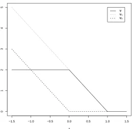
We now intuitively explain advantages of ˆU(f) over a popular large margin loss L(|f|) = (1− |f(x)|)+(Vapnik, 1998; Wang and Shen, 2007), and its connection with the clustering assumption (Chapelle and Zien, 2005) that assumes closeness between the classification and grouping (cluster-ing) boundaries.
First, ˆU(f)has an optimality property, as discussed in Section 2.2, which leads to better perfor-mance as suggested by Theorem 3. Second, it has a higher discriminative power over its counterpart
L(|f|). To see this aspect, note that L(|f|) =infpU(f)by Lemma 1 of Wang and Shen (2007). This
the dashed line. By comparison, ˆU(f)enables not only to identify the clustering boundary through the hat function as L(|f|)does but also to discriminate f(x)from−f(x)through an estimated ˆp(x). That is, ˆU(f) has a smaller value for f(x)>0 than for −f(x)<0 when ˆp>0.5, and vice versa, whereas L(|f|)is in-discriminative with regard to the sign of f(x).
−2 −1 0 1 2
f(x)
U(f(x))
0
1−p
^
p^
1
L(|f(x)|) U^(f(x))
Figure 1: Plots of L(|f(x)|)and ˆU(f(x)).
To reinforce the second point in the foregoing discussion, we examine one specific example with two possible clustering boundaries as described in Figure 3 of Zhu (2005). There ˆU(f)favors one clustering boundary for classification if a consistent ˆp is provided, whereas L(|f|)fails to dis-criminate these two. More details are deferred to Section 4.1, where the simulated example 2 of this nature is studied.
In conclusion, ˆU(f) yields a more efficient loss for a semisupervised problem as it uses the clustering information from the unlabeled data as L(|f|)does, in addition to guidance about labeling through ˆp to gain a higher discriminative power.
3. Computation
In this section, we implement the proposed semisupervised method through an iterative scheme as well as a nonconvex optimization technique.
3.1 Iterative Scheme
been used in estimation of ˆf(1)through ˆp(0)and additional smoothness structure has been used in Algorithm 0 in estimation of ˆp(1)given ˆf(1). Specifically, an improvement in the process from ˆp(0)
to ˆf(1)and that from ˆf(1)to ˆp(1)are assured by Assumptions B and D in Section 5.1, respectively, which are a more general version of the clustering assumption and a smoothness assumption of p. In other words, the marginal information from unlabeled data has been effectively incorporated in each iteration of Algorithm 1 for improving estimation accuracy of ˆf and ˆp.
Detailed implementation of the preceding scheme as well as the conditional probability estima-tion are summarized as follows.
Algorithm 0: (Conditional probability estimation; Wang, Shen and Liu, 2008)
Step 1. Specify m and initializeπt = (t−1)/m, for t=1, . . . ,m+1. Step 2. Train weighted margin classifiers ˆfπt by solving
min
f∈F Cn
−1 (1
−πt)
∑
yi=1L(yif(xi)) +πt
∑
yi=−1L(yif(xi))
!
+J(f),
with 1−πt associated with positive instances andπt associated with negative instances. Step 3. Estimate labels of x by sign(fˆπt(x)).
Step 4. Sort sign{fˆπt(x)}, t =1, . . . ,m+1, to compute π∗=max
πt : sign(fˆπt(x)) =1 , π∗=
minπt : sign(fˆπt(x)) =−1 . The estimated class probability is ˆp(x) =
1
2(π∗+π∗). Algorithm 1: (Efficient semisupervised learning)
Step 1. (Initialization) Given any initial classifier sign(fˆ(0)), compute ˆp(0) through Algorithm 0. Specify precision tolerance levelε.
Step 2. (Iteration) At iteration k+1; k=0,1,···, minimize s(f) in (2) for ˆf(k+1) with ˆU =Uˆ(k) defined by ˆp= pˆ(k) there. This is achieved through sequential QP for the ψ-loss. Details for sequential QP are deferred to Section 3.2. Compute ˆ˜p(k+1)through Algorithm 0, based on complete data with unknown labels imputed by sign(fˆ(k+1)). Define ˆp(k+1)=max(pˆ(k),ˆ˜p(k+1))when ˆf(k+1)≥ 0 and min(pˆ(k),ˆ˜p(k+1))otherwise.
Step 3. (Stopping rule) Terminate when|s(fˆ(k+1))−s(fˆ(k))| ≤ε|s(fˆ(k))|. The final solution ˆfC is
ˆ
f(K), with K the number of iterations to termination in Algorithm 1.
Theorem 2 (Monotonicity) s(fˆ(k)) is non-increasing in k. As a consequence, Algorithm 1
con-verges to a stationary point s(fˆ(∞)) in that s(fˆ(k))≥s(fˆ(∞)). Moreover, Algorithm 1 terminates finitely.
Algorithm 1 differs from the EM algorithm and its variant MM algorithm (Hunter and Lange, 2000) in that little marginal information has been used in these algorithms as argued in Zhang and Oles (2000). Algorithm 1 also differs from Yarowsky’s algorithm (Yarowsky, 1995; Abney, 2004) in that Yarowsky’s algorithm solely relies on the strength of the estimated ˆp, ignoring the potential
information from the clustering assumption.
Finally, we note that in Step 2 of Algorithm 1, given ˆp(k), minimization in (2) involves non-convex minimization when L(·)isψ-loss. Next we shall discuss how to solve (2) for ˆf(k+1)through difference convex (DC) programming for nonconvex minimization.
3.2 Nonconvex Minimization
This section develops a nonconvex minimization method based on DC programming (An and Tao, 1997) for (2) with the ψ-loss, which was previously employed in Liu, Shen and Wong (2005) for supervisedψ-learning. As a technical remark, we note that DC programming has a high chance to locate anε-global minimizer (An and Tao, 1997), although it can not guarantee globality. In fact, when combined with the method of branch-and-bound, it yields a global minimizer, see Liu et al. (2005). For a computational consideration, we shall use the DC programming algorithm without seeking an exact global minimizer.
Key to DC programming is decomposing the cost function s(f)in (2) with L(z) =ψ(z) into a difference of two convex functions as follows:
s(f) = s1(f)−s2(f); (3)
s1(f) = C n−l 1 nl
∑
i=1
ψ1(yif(xi)) +n−u1 n
∑
j=nl+1 ˆ
Uψ(k1)(f(xj))
+J(f);
s2(f) = C n−l 1 nl
∑
i=1
ψ2(yif(xi)) +n−u1 n
∑
j=nl+1 ˆ
Uψ(k2)(f(xj))
,
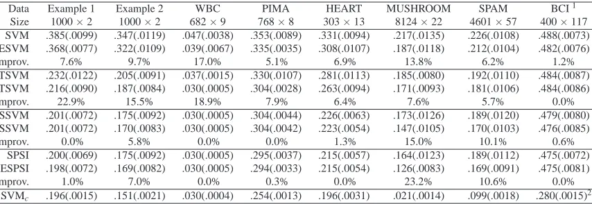
where ˆUψ(kt)(f(xj)) = pˆ(k)(xj)ψt(f(xj)) + (1−pˆ(k)(xj))ψt(−f(xj)); t =1,2, ψ1=2(1−z)+ and
ψ2=2(−z)+. Hereψ1 andψ2 are obtained through a convex decomposition ofψ=ψ1−ψ2 as displayed in Figure 2.
With these decompositions, we treat (2) with theψ-loss and ˆp=pˆ(k)by solving a sequence of quadratic problems described in Algorithm 2.
Algorithm 2: (Sequential QP)
Step 1. (Initialization) Set initial ˆf(k+1,0)to be the solution of minfs1(f). Specify precision
toler-ance levelεas in Algorithm 1.
Step 2. (Iteration) At iteration l+1, compute ˆf(k+1,l+1)by solving min
f s1(f)− hwf,∇s2(
ˆ
f(k+1,l))i
, (4)
where∇s2(f(k+1,l))is a gradient vector of s2(f)at wfˆ(k+1,l).
Step 3. (Stopping rule) Terminate when|s(fˆ(k+1,l+1))−s(fˆ(k+1,l))| ≤ε|s(fˆ(k+1,l))|. Then the estimate ˆf(k+1)is the best solution among ˆf(k+1,l); l=0,1,···.
In (4), gradient∇s2(f(k+1,l))is defined as the sum of partial derivatives of s2over each observa-tion, with∇ψ2(z) =0 if z>0 and∇ψ2(z) =−2 otherwise. By the definition of∇s2(f(k+1,l))and convexity of s2(f(k+1,l)), (4) gives a sequence of non-increasing upper envelops of (3), which can be solved via their dual forms.
−1.5 −1.0 −0.5 0.0 0.5 1.0 1.5
0
1
2
3
4
5
z
ψ ψ1
ψ2
Figure 2: Plot ofψ,ψ1andψ2for the DC decomposition ofψ=ψ1−ψ2. Solid, dotted and dashed lines representψ,ψ1andψ2, respectively.
4. Numerical Comparison
This section examines effectiveness of the proposed method through numerical examples. A test error, averaged over 100 independent simulation replications, is used to measure a classifier’s gen-eralization performance. For simulation comparison, the amount of improvement of our method over sign(fˆ(0))is defined as the percent of improvement in terms of the Bayesian regret
(T(Before)−Bayes)−(T(After)−Bayes)
T(Before)−Bayes , (5)
where T(Before), T(After), and Bayes denote the test errors of sign(fˆ(0)), the proposed method based on initial classifier sign(fˆ(0)), and the Bayes error. The Bayes error is the ideal performance and serves as a benchmark for comparison, which can be computed when the distribution is known. For benchmark examples, the amount of improvement over sign(fˆ(0))is defined as
T(Before)−T(After)
T(Before) , (6)
which actually underestimates the amount of improvement in absence of knowledge of the Bayes error.
4.1 Simulations and Benchmarks
Two simulated and five benchmark data sets are examined, based on four state-of-the-art classifiers sign(fˆ(0))’s. They are SVM (with labeled data alone), TSVM (TSVMDCA; Wang, Shen and Pan,
2007) , and the methods of Wang and Shen (2007) with the hinge loss (SSVM) and with theψ -loss (SPSI), where SSVM and SPSI compare favorably against their competitors. Corresponding to these methods, our method, with m=n1/2 andε=10−3, yields four semisupervised classifiers denoted as ESVM, ETSVM, ESSVM and ESPSI.
4.1.1 SIMULATEDEXAMPLES
Examples 1 and 2 are taken from Wang and Shen (2007), where 200 and 800 labeled instances are randomly selected for training and testing. For training, 190 out 200 instances are randomly chosen for removing their labels. Here the Bayes errors are 0.162 and 0.089, respectively.
4.1.2 BENCHMARKS
Six benchmark examples include Wisconsin breast cancer (WBC), Pima Indians diabetes (PIMA), HEART, MUSHROOM, Spam email (SPAM) and Brain computer interface (BCI). The first five datasets are available in the UCI Machine Learning Repository (Blake and Merz, 1998) and the last one can be found in Chapelle et al. (2006). WBC discriminates a benign breast tissue from a malignant one through 9 diagnostic characteristics; PIMA differentiates between positive and negative cases for female diabetic patients of Pima Indian heritage based on 8 biological or diag-nostic attributes; HEART concerns diagnosis status of the heart disease based on 13 clinic attributes; MUSHROOM separates an edible mushroom from a poisonous one through 22 biological records; SPAM identifies spam emails using 57 frequency attributes of a text, such as frequencies of partic-ular words and characters; BCI concerns the difference of brain images when imagining left-hand and right-hand movements, based on 117 autoregressive model parameters fitted over human’s elec-troencephalography.
Instances in WBC, PIMA, HEART, and MUSHROOM are randomly divided into two halves with 10 labeled and 190 unlabeled instances for training, and the remaining 400 for testing. In-stances in SPAM are randomly divided into halves with 20 labeled and 380 unlabeled inIn-stances for training, and the remaining instances for testing. Twelve splits for BCI have already given at http://www.kyb.tuebingen.mpg.de/ssl-book/benchmarks.html, with 10 labeled and 390 unlabeled instances while no instance for testing. An averaged error rate over the unlabeled set is used in BCI example to approximate the test error.
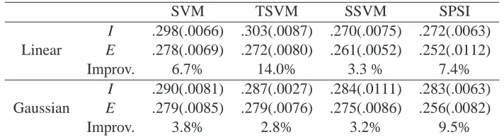
In each example, the smallest test errors of all methods in comparison are computed over 61 grid points{10−3+k/10; k=0,···,60} for tuning C in (2) through a grid search. The results are summarized in Tables 1-2.
improve-Data Example 1 Example 2 WBC PIMA HEART MUSHROOM SPAM BCI1 Size 1000×2 1000×2 682×9 768×8 303×13 8124×22 4601×57 400×117 SVM .345(.0081) .333(.0129) .053(.0071) .328(.0092) .284(.0085) .232(.0135) .216(.0097) .479(.0059) ESVM .281(.0143) .297(.0177) .031(.0007) .320(.0059) .214(.0066) .172(.0084) .217(.0178) .474(.0052)
Improv. 35.0% 14.8% 41.5% 2.4% 24.6% 25.9% -0.5% 1.0%
TSVM .220(.0103) .203(.0088) .037(.0024) .314(.0086) .270(.0082) .206(.113) .196(.0132) .479(.0054) ETSVM .190(.0074) .147(.0131) .029(.0009) .309(.0063) .211(.0062) .153(.0054) .179(.0101) .474(.0076)
Improv. 51.7% 49.1% 21.6% 1.6% 21.9% 25.7% 8.7% 1.0%
SSVM .188(.0084) .129(.0031) .032(.0025) .307(.0054) .240(.0074) .186(.0095) .191(.0114) .479(.0071) ESSVM .182(.0065) .124(.0034) .028(.0006) .293(.0029) .205(.0059) .162(.0054) .169(.0107) .474(.0041)
Improv. 23.1% 12.5% 12.5% 4.6% 14.6% 11.8% 11.5% 1.0%
SPSI .184(.0084) .128(.0084) .029(.0022) .291(.0032) .232(.0067) .184(.0095) .189(.0107) .476(.0068) ESPSI .182(.0065) .123(.0029) .027(.0006) .284(.0026) .181(.0052) .137(.0067) .167(.0107) .471(.0046)
Improv. 9.1% 12.8% 6.9% 2.4% 22.0% 25.5% 11.6% 1.1%
SVMc .164(.0084) .115(.0032) .027(.0020) .238(.0011) .176(.0031) .041(.0018) .095(.0022) .173(.0012)2
Table 1: Linear learning. Averaged test errors as well as estimated standard errors (in parenthesis) of ESVM, ETSVM, ESSVM, ESPSI, and their initial counterpartsand testing samples, in the simulated and benchmark examples. SVMc denotes the performance of SVM with
complete labeled data. Here the amount of improvement is defined in (5) or (6).
Data Example 1 Example 2 WBC PIMA HEART MUSHROOM SPAM BCI1
Size 1000×2 1000×2 682×9 768×8 303×13 8124×22 4601×57 400×117 SVM .385(.0099) .347(.0119) .047(.0038) .353(.0089) .331(.0094) .217(.0135) .226(.0108) .488(.0073) ESVM .368(.0077) .322(.0109) .039(.0067) .335(.0035) .308(.0107) .187(.0118) .212(.0104) .482(.0076)
Improv. 7.6% 9.7% 17.0% 5.1% 6.9% 13.8% 6.2% 1.2%
TSVM .232(.0122) .205(.0091) .037(.0015) .330(.0107) .281(.0113) .185(.0080) .192(.0110) .484(.0087) ETSVM .216(.0090) .187(.0084) .030(.0005) .304(.0028) .263(.0094) .171(.0093) .181(.0106) .484(.0086)
Improv. 22.9% 15.5% 18.9% 7.9% 6.4% 7.6% 5.7% 0.0%
SSVM .201(.0072) .175(.0092) .030(.0005) .304(.0044) .226(.0063) .173(.0126) .189(.0120) .479(.0080) ESSVM .201(.0072) .170(.0083) .030(.0005) .304(.0042) .223(.0054) .147(.0105) .170(.0103) .476(.0085)
Improv. 0.0% 5.8% 0.0% 0.0% 1.3% 15.0% 10.1% 0.6%
SPSI .200(.0069) .175(.0092) .030(.0005) .295(.0037) .215(.0057) .164(.0123) .189(.0112) .475(.0072) ESPSI .198(.0072) .169(.0082) .030(.0005) .294(.0033) .215(.0054) .126(.0083) .169(.0091) .475(.0081)
Improv. 1.0% 7.0% 0.0% 0.3% 0.0% 23.2% 10.6% 0.0%
SVMc .196(.0015) .151(.0021) .030(.0004) .254(.0013) .196(.0031) .021(.0014) .099(.0018) .280(.0015)2
Table 2: Gaussian kernel learning. Averaged test errors as well as estimated standard errors (in parenthesis) of ESVM, ETSVM, ESSVM, ESPSI, and their initial counterpartsin the sim-ulated and benchmark examples. Here the amount of improvement is defined in (5) or (6).
ment becomes small or null, such as the cases of SSVM and SPSI with Gaussian kernel in PIMA. If the initial classifier is too poor, then no improvement may occur. This is the case for ESVM with linear kernel in SPAM, where ESVM performs worse than SVM with nl =10 labeled data alone.
This suggests that a better initial estimate should be used together with unlabeled data.
In summary, we recommend SPSI to be an initial classifier for ˆf(0)based on its overall perfor-mance across all the examples. Moreover, ESPSI nearly recovers the classification perforperfor-mance of its counterpart SVM with complete labeled data in the two simulated examples, WBC and HEART.
4.2 Gene Function Prediction Through Expression Profiles
This section applies the proposed method to predict gene functions through gene data in Hughes et al. (2000), consisting of expression profiles of a total of 6316 genes for yeast S. cerevisiae from
300 microarray experiments. In this case almost half of the genes have unknown functions although gene expression profiles are available for almost the entire yeast genome.
Our specific focus is predicting functional categories defined by the MIPS, a multifunctional classification scheme (Mewes et al., 2002). For simplicity, we examine two functional categories, namely “transcriptional control” and “mitochondrion”, with 334 and 346 annotated genes, respec-tively. The goal is to predict gene functional categories for genes annotated within these two cate-gories by training our semisupervised classifier on expression profiles of genes, where some genes are treated as if their functions are unknown to mimic the semisupervised scenario in complete dataset. At present, detection of novel class is not permitted in our formulation, which remains to be an open research question.
For the purpose of evaluation, we divide the entire dataset into two sets of training and testing. The training set involves a random sample of nl=20 labeled and nu=380 unlabeled gene profiles,
while the testing set contains 280 remaining profiles.
SVM TSVM SSVM SPSI
I .298(.0066) .303(.0087) .270(.0075) .272(.0063) Linear E .278(.0069) .272(.0080) .261(.0052) .252(.0112)
Improv. 6.7% 14.0% 3.3 % 7.4%
I .290(.0081) .287(.0027) .284(.0111) .283(.0063) Gaussian E .279(.0085) .279(.0076) .275(.0086) .256(.0082)
Improv. 3.8% 2.8% 3.2% 9.5%
Table 3: Averaged test errors as well as estimated standard errors (in parenthesis) of ESVM, ETSVM, ESSVM, ESPSI, and their initial counterparts, over 100 pairs of training and testing samples, in gene function prediction. Here I stands for an initial classifier, E stands for our proposed method with the initial method, and the amount of improvement is de-fined in (6).
As indicated in Table 3, ESVM, ETSVM, ESSVM and ESPSI all improve predictive accuracy of their initial counterparts in linear learning and Gaussian kernel learning. It appears that ESPSI performs best. Most importantly, it demonstrates predictive power of the proposed method for predicting which of the two categories a gene belongs to.
5. Statistical Learning Theory
In the literature, several theories have been developed to understand the problem of semisuper-vised learning, including Rigollet (2007) and Singh, Nowak and Zhu (2008). Both the theories rely on a different clustering assumption that homogeneous labels are assumed over local clusters. Based on the original clustering assumption, as well as a smoothness assumption on the condi-tional probability p(x), this section develops a novel statistical learning theory. Specifically, finite-sample and asymptotical upper bounds of the generalization error are derived for ESPSI ˆfCdefined
by the ψ-loss in Algorithm 1. The generalization accuracy is measured by the Bayesian regret
5.1 Statistical Learning Theory
The error bounds of e(fˆC,f¯.5) are expressed in terms of complexity of the candidate class
F
, the sample size n, tuning parameter λ= (nC)−1, the error rate of the initial classifier δ(0)n , and the
maximum number of iteration K in Algorithm 1. The results imply that ESPSI, without knowing labels of the unlabeled data, enables to recover the classification accuracy ofψ-learning based on complete data under regularity conditions.
We first introduce some notations. Let L(z) =ψ(z) be the ψ-loss. Define the margin loss
Vπ(f,Z)for unequal cost classification to be Sπ(y)L(y f(x)), with cost 0<π<1 for the positive class and Sπ(y) =1−π if y=1, andπ otherwise. Let eVπ(f,f¯π)E(Vπ(f,Z)−Vπ(f¯π,Z))≥0 for
f ∈
F
with respect to unequal costπ, where ¯fπ(x) =sign(fπ(x)) =arg minfEVπ(f,Z)is the Bayesrule, with fπ(x) =p(x)−π.
Assumption A: (Approximation) For anyπ∈(0,1), there exist some positive sequence sn→0 as n→∞and fπ∗∈
F
such that eVπ(fπ∗,f¯π)≤sn.Assumption A is an analog of that of Shen et al. (2003), which ensures that the Bayes rule ¯fπ
can be well approximated by elements in
F
.Assumption B. (Conversion) For anyπ∈(0,1), there exist constants 0<α, βπ<∞, 0≤ζ<∞,
ai>0; i=0,1,2, such that for any sufficiently smallδ>0,
sup
{f∈F:eV.5(f,f¯.5)≤δ}
e(f,f¯.5) ≤ a0δα, (7) sup
{f∈F:eVπ(f,f¯π)≤δ}
ksign(f)−sign(f¯π)k1 ≤ a1δβπ, (8) sup
{f∈F:eVπ(f,f¯π)≤δ}
Var(Vπ(f,Z)−Vπ(f¯π,Z)) ≤ a2δζ. (9)
Assumption B describes local smoothness of the Bayesian regret e(f,f¯.5) in terms of a first-moment function ksign(f)−sign(f¯π)k1 and a second-moment function Var(Vπ(f,Z) −Vπ(f¯π,Z)) relative to eVπ(f,f¯π)with respect to unequal costπ. Here the degrees of smoothness are defined by
exponentsα,βπandζ. Note that (7) and (9) are related to the “no noise assumption” of Tsybakov (2004); and (8) has been used in Wang et al. (2008) for quantifying the error rate of probability estimation, which plays a key role in controlling the error rate of ESPSI. For simplicity, denoteβ.5 and infπ6=0.5{βπ}asβandγrespectively, whereβquantifies the clustering assumption through the degree to which the positive and negative clusters are distinguishable, andγmeasures the conversion rate between the classification and probability estimation accuracies.
For Assumption C, we define a complexity measure—the L2-metric entropy with bracketing, describing the cardinality of
F
. Given anyε>0, denote{(frl,fru)}Rr=1as anε-bracketing function set of
F
if for any f ∈F
, there exists an r such that frl≤ f ≤ fruandkfrl−fruk2≤ε; r=1,···,R.Then the L2-metric entropy with bracketing HB(ε,
F
)is defined as the logarithm of the cardinalityof the smallestε-bracketing function set of
F
. See Kolmogorov and Tihomirov (1959) for more details.Define
F
(k) ={L(f,z)−L(fπ∗,z): f∈F
,J(f)≤k}to be a space defined by candidate decision functions, with J(f) = 12kfk2K. Let Jπ∗=max(J(fπ∗),1). In (11), we specify an entropy integral to
establish a relationship between the complexity of
F
(k)and convergence speedεnfor the BayesianAssumption C. (Complexity) For some constants ai>0; i=3,···,5 andεn>0,
sup
k≥2
φ(εn,k)≤a5n1/2, (10)
whereφ(ε,k) =Ra
1/2 3 M
min(1,ζ)/2
a4M H
1/2
B (w,
F
(k))dw/M, and M=M(ε,λ,k) =min(ε2+λ(k/2−1)Jπ∗,1).Assumption D. (Smoothness of p(x)) There exist some constants 0≤η≤1, d≥0 and a6>0 such thatk∆j(p)k∞≤a6 for j=0,1,···,d, and|∆d(p(x1))−∆d(p(x2))| ≤a6kx1−x2kη1+d/m for any kx1−x2k1≤δ with some sufficiently smallδ>0, where∆j is the j-th order difference operator and m is defined as in Algorithm 0.
Assumption D specifies the degree of smoothness of the conditional density p(x).
Assumption E. (Degree of least favorable situation) There exist some constants 0≤θ≤∞and
a7>0 such that P X : min(p(X),1−p(X))≤δ
≤a7δθfor any sufficiently smallδ>0.
Assumption E describes the behavior of p(x)near 0 and 1, corresponding to the least favorable situation, as described in Section 2.3.
Theorem 3 In addition to Assumptions A-E, let the precision parameter m be [δ−nβγ] and δ2n=
min(max(ε2
n,16sn),1). Then for ESPSI ˆfC, there exist some positive constants a8-a10such that
Pe(fˆC,f¯.5)≥a10max(δ2α
n ,(a11ρnδn(0))2αmax(1,B K)
)≤
P
eL(fˆ.(50),f¯.5)≥2a11ρn(δ(n0))2
+3.5K exp(−a8nl(λJ.∗5)max(1,2−ζ))+ 3.5K exp(−a9n(λJπ∗)max(1,2−ζ)) +2Kρ−
min(1,β)
n .
Here B=2(1+max(θ+(01,1)(−dβ+)θη)()βγd+η+1), a11=max
1,2 3γ(d+η)
d+η+1+2a
(2γ+1)(d+η)
d+η+1 1
andρn>0 is any real number satisfying a11ρnδ2n≤4λJπ∗.
Theorem 3 provides a finite-sample probability bound for the Bayesian regret e(fˆC,f¯.5), where the parameter B measures the level of difficulty of a semisupervised problem, with small value of B indicating more difficulty. Note that the value of B is proportional to those ofα,β,γ, d,ηandθ, as defined in Assumptions A-E. In fact,α,βandγquantify the local smoothness of the Bayesian regret e(f,f¯.5), and d,ηandθdescribe the smoothness of p(x)as well as its behavior near 0 and 1. Next, by letting nl,nutending infinity, we obtain the rates of convergence of ESPSI in terms of
the error rateδ2α
n of its supervised counterpartψ-learning based on complete data, and the initial
error rateδ(n0), B, and the maximum number K of iteration.
Corollary 4 Under the assumptions of Theorem 3, as nu,nl →∞,
|e(fCˆ ,f¯.5)| = Op
max(δ2nα,(ρnδn(0))2αmax(1,B K)
),
E|e(fˆC,f¯.5)| = Omax(δ2α
n ,(ρnδn(0))2αmax(1,B K)
),
provided that the initial classifier converges in that P
eL(fˆ.(50),f¯.5)≥2a11ρn(δ(n0))2
→0, with any
slow varying sequence ρn→∞andρnδ(n0)→0, and the tuning parameter λ is chosen such that n(λJπ∗)max(1,2−ζ)and n
Note that there are two important cases defined by the value of B. When B>1, ESPSI achieves the convergence rateδ2nαof its supervised counterpartψ-learning based on complete data, c.f., The-orem 1 of (Shen and Wang, 2007). When B≤1, ESPSI performs no worse than its initial classifier because(δ(n0))2αmax(1,B
K)
(δ(n0))2α. Therefore, it is critical to compute the value of B. For instance,
if the two classes are perfectly separated and located very densely within respective regions, then
B=∞and our method recovers the rate δ2nα; if the two classes are completely indistinguishable, then B=0 and our method yields the rate(δ(n0))2.
For the optimality claimed in Section 2.2, we show that ˆU(f)is sufficiently close to U(f)so that optimality of U(f)can be translated into ˆU(f). As a result, minimization of ˆU(f)over f mimics that of U(f).
Corollary 5 (Optimality) Under the assumptions of Corollary 4, as nu,nl→∞,
sup
f∈Fk
ˆ
U(f)−U(f)k1 = Op
max(δβγn ,(ρnδn(0))βγmax(1,B K)
),
where ˆU(f)is estimated U(f)loss with p estimated based on ˆfC.
To argue that the approximation error rate of ˆU(f) to U(f) is sufficiently small, note that ˆfC
obtained from minimizing (2) recovers the classification error rate of its supervised counterpart based on complete data, as suggested by Corollary 4. Otherwise, a poor approximation precision could impede the error rate of ESPSI.
In conclusion, ESPSI, without knowing label values of unlabeled instances, enables to recon-struct the classification and estimation performance ofψ-learning based on complete data in rates of convergence, when possible.
5.2 Theoretical Example
We now apply Corollary 4 to linear and kernel learning examples to derive generalization errors rates for ESPSI in terms of the Bayesian regret. In all cases, ESPSI (nearly) achieves the generalization error rates ofψ-learning for complete data when unlabeled data provides useful information, and yields no worse performance then its initial classifier otherwise.
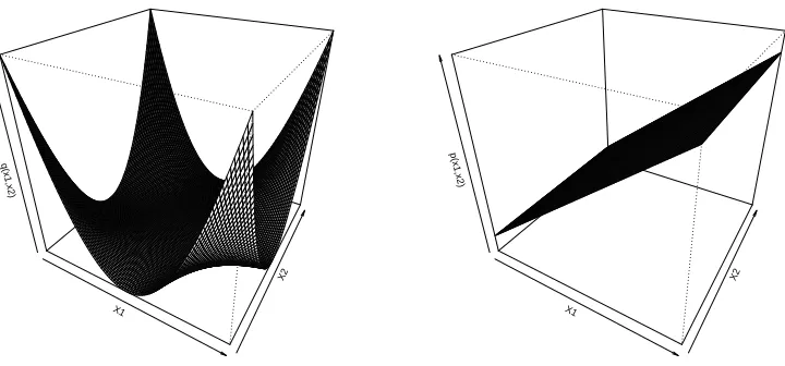
Consider a learning example in which X = (X·1,X·2)are independent, following marginal dis-tribution q(x) = 12(κ1+1)|x|κ1 for x∈[−1,1]forκ1>0. Given X =1, P(Y =1|X=x) =p(x) =
2
5sign(x·1)|x·1|κ2+ 1
2 withκ2>0. Note that fπ(x) is x·1−sign(π− 1 2)(
5
4|2π−1|) 1
κ2, which in turn yields the vertical line as the decision boundary for classification with unequal costπ. The value ofκi; i=1,2 describe the behavior of the marginal distribution around the origin, and that of the
conditional distribution p(x)in the neighborhood of 1/2, respectively.
For illustration, Figure 3 displays the marginal and conditional densities from the data distribu-tion withκ1=2 andκ2=1. It is evident that the clustering assumption (Assumption B) is met since the neighborhood of f.5(x) has low density as showed in the left panel of Figure 3, and the smoothness assumption (Assumption D) and the boundedness assumption of p(x) (Assumption E) are met as well since p(x)is a hyperplane bounded by(0.1,0.9)as showed in the right panel of Figure 3. Technical details of verifying assumptions are deferred to Appendix B.
5.2.1 LINEARLEARNING
Here it is natural to consider linear learning in which candidate decision functions are linear in
X1
X2 q(x1,x2)
X1
X2 p(x1,x2)
Figure 3: Plots of the marginal and conditional densities from the data distribution withκ1=2 and
κ2=1.
For ESPSI ˆfC, we chooseδ(n0)=n−l 1log nl, the convergence rate of supervised linearψ-learning, ρn→∞to be an arbitrarily slow sequence and C=O((log n)−1). An application of Corollary 4
yields that E|e(fCˆ ,f¯.5)|=O(max(n−1log n,(n−l 1(log nl)2)max(1,2B K)
)), with B= (1+κ1)2
2κ2(1+κ1+κ2). When
B>1, equivalently,κ1+1>(1+ √
3)κ2, this rate reduces to O(n−1log n)when K is sufficiently large. Otherwise, the rate is O(n−l 1log nl).
The fast rate n−1log n is achieved when κ1 is large but κ2 is relatively small. Interestingly, largeκ1 value implies that q(x)has a low density around x=0, corresponding to the low density separation assumption in Chapelle and Zien (2005) for a semisupervised problem, whereas large
κ1 value and smallκ2 value indicate that p(x)has a small probability to be close to the decision boundary p(x) =1/2 for a supervised problem.
5.2.2 KERNELLEARNING
Consider a flexible representation defined by a Gaussian kernel, where
F
={x∈R
2: f(x)wf,0+∑n
k=1wf,kK(x,xk): wf = (wf,1,···,wf,n)T ∈
R
n} by the representation theorem of RKHS, seeWahba (1990). Here K(x,z) =exp(−kx2−σz2k2)is the Gaussian kernel.
Similarly, we choose δ(n0)=nl−1(log nl)3 to be the convergence rate of supervised ψ-learning
with Gaussian kernel,ρn→∞to be an arbitrarily slow sequence and C=O((log n)−3). By Corollary
4, E|e(fˆC,f¯.5)|=O(max((n−1
l (log nl)3)max(1,2B K)
,n−1(log n)3)) =O(n−1(log n)3) when κ 1+1> 2κ2(1+κ2)and K is sufficiently large, and O(nl−1(log nl)3) otherwise. Again, largeκ1 and small
6. Summary
This article introduces a large margin semisupervised learning method through an iterative scheme based on an efficient loss for unlabeled data. In contrast to most methods assuming a relationship between the conditional and the marginal distributions, the proposed method integrates labeled and unlabeled data through using the clustering structure of unlabeled data as well as the smoothness structure of the estimated p. The theoretical and numerical results suggest that the method compares favorably against top competitors, and achieves the desired goal of reconstructing the classification performance of its supervised counterpart on complete labeled data.
With regard to tuning parameter C, further investigation is necessary. One critical issue is how to use unlabeled data to enhance the accuracy of estimating the generalization error so that adaptive tuning is possible.
Acknowledgments
This research is supported in part by NSF grants IIS-0328802 and DMS-0604394, by NIH grants HL65462 and 1R01GM081535-01, and a UM AHC FRD grant.
Appendix A. Technical Proofs
Proof of Lemma 1: Let U(f(x)) = E(L(Y f(X))|X = x). By orthogonality, E(L(Y f(X))−
T(f(X)))2=E(L(Y f(X))−U(f(X)))2+E(U(f(X))−T(f(X)))2, implying that U(f(x)) mini-mizes E(L(Y f(X))−T(f(X)))2over any T . Then the proof follows from the fact that EL(Y f(X)) =
E(E(L(Y f(X))|X)).
Proof of Theorem 2: For clarity, we write s(fˆ)as s(fˆ,pˆ)in this proof. Then it suffices to show that
s(fˆ(k),pˆ(k))≥s(fˆ(k+1),pˆ(k+1)). First, s(fˆ(k),pˆ(k))≥s(fˆ(k+1),pˆ(k))since ˆf(k+1)minimizes s(f,pˆ(k)). Then s(fˆ(k+1),pˆ(k))−s(fˆ(k+1),pˆ(k+1)) =∑n
j=nl+1(pˆ(k)−pˆ(k+1))(L(fˆ(k+1)(xj))−L(−fˆ(k+1)(xj))),
which is nonnegative by the definition of ˆp(k+1).
Proof of Theorem 3: The proof involves two steps. In Step 1, given f(k), we derive a probability upper bound for kpˆ(k)−pk1, where ˆp(k) is obtained from Algorithm 0. In Step 2, based on the result of Step 1, the difference between the tail probability of eπ(fˆ(k+1)
π ,f¯π)and that of eπ(fˆ(k)
π ,f¯π)
is bounded through a large deviation inequality of Wang and Shen (2007); k=0,1,···. This in turn results in a faster rate for e(fˆ(k+1)
.5 ,f¯.5), thus e(fCˆ ,f¯.5). In this proof, we denote labeled and unlabeled samples by{(Xi,Yi)}nli=1and{Xj}nj=nl+1to indicate that they are all random variables.
Step 1: First we bound the probability of the percentage of wrongly labeled unlabeled instances by sign(fˆ(k))by the tail probability of eV.5(fˆ
(k),f¯
.5). For this purpose, define Df={sign(fˆ(k)(Xj))6=
sign(f¯.5(Xj)); nl+1≤ j≤n}to be the set of unlabeled data that are wrongly labeled by sign(fˆ(k)),
with nf =#{Df} being its cardinality. According to Markov’s inequality, the fact that E( nf
n) = nu
nEksign(fˆ(
k+1))−sign(f¯
.5)k1, and (8), we have
Pnf
n ≥a1(a11ρ
2
n(δ
(k)
n )2)β
≤ Pksign(fˆ(k))−sign(f¯
.5)k1≥a1(a11ρn(δ(nk))2)β
+Pnf n ≥ρ
β
nksign(fˆ(k+1))−sign(f¯.5)k1
≤ P
eV.5(fˆ (k),f¯
.5)≥a11ρn(δ(nk))2
Next we bound the tail probability ofkpˆ(k)−pk1 based on “complete” data consisting of un-labeled data assigned by sign(fˆ(k)). An application of similar treatment to that in the proof of Theorem 3 of Wang et al. (2008) leads to
Pkpˆ(k)−pk1≥8γa12γ+1(a11ρnδ(nk))βγ
≤
P(∃j :ksign(fˆπ(kj))−sign(f¯πj)k1≥8
γa2γ+1
1 (a11ρnδ (k)
n )2βγ),
(12)
withπj= j/⌈(a11ρnδn(k))−βγ⌉. By (8), it suffices to bound P(eVπ(fˆ
(k)
πj ,f¯πj)≥8a
2
1(a11ρnδ(nk))2β)for
allπj in what follows.
We introduce some notations to be used. Let ˜Vπ(f,Z) =Vπ(f,Z) +λJ(f), and Zj= (Xj,Yj)with Yj =sign(fˆ(k)(Xj)); nl+1≤ j≤n. Define a scaled empirical process En(V˜π(fπ∗,Z)−V˜π(f,Z)) = n−1
∑i∈Df+∑i∈/Df
˜
Vπ(fπ∗,Zi)−V˜π(f,Zi)−E(V˜π(fπ∗,Zi)−V˜π(f,Zi))≡En(Vπ(fπ∗,Z)−Vπ(f,Z)).
By the definition of ˆfπ(k)and (11),
PeVπ(fˆπ(k),f¯π)≥δ2k
≤ Pnf
n ≥a1(a11ρ 2
n(δ
(k)
n )2)β
+
P∗sup
Nk
1 n
n
∑
i=1(V˜π(f∗
π,Zi)−V˜π(f,Zi))≥0,
nf
n ≤a1(a11ρ 2
n(δ
(k)
n )2)β
≤ PeV.5(fˆ (k),f¯
.5)≥a11ρn(δ(nk))2
+ρ−nβ+I1, (13)
where Nk ={f ∈
F
: eVπ(f,f¯π)≥δ2k}, δ2k =8a21(a11ρnδ(nk))2β, I1 =P∗
supNkEn(Vπ(fπ∗, Z)−
Vπ(f,Z))≥infNk∇(f,fπ∗),nfn ≤a1(a11ρ2n(δ
(k)
n )2)β
, and∇(f,fπ∗) =nf
nEi∈Df(V˜π(f,Zi)−V˜π(fπ∗,Zi))+ n−nf
n Ei∈/Df(V˜π(f,Zi)−V˜π(fπ∗,Zi)).
To bound I1, we partition Nkinto a union of As,t with
As,t = {f ∈
F
: 2s−1δ2k≤eVπ(f,f¯π)<2sδ2k,2t−1Jπ∗≤J(f)<2tJπ∗}; As,0 = {f ∈F
: 2s−1δ2k≤eVπ(f,f¯π)<2sδ2k,J(f)<Jπ∗},for s,t=1,2,···. Then it suffices to bound the corresponding probability over each As,t. Toward this
end, we need to bound the first and second moments of ˜Vπ(f,Z)−V˜π(f∗
π,Z)over f ∈As,t. Without
loss of generality, assume that 4sn<δ2k<1, J(fπ∗)≥1, and thus Jπ∗=max(J(fπ∗),1) =J(fπ∗).
For the first moment, note that∇(f,fπ∗)≥eVπ(f,fπ∗)−
nf
nE|Vπ(f,Z)−Vπ(fπ∗,Z) +V¯π(f,Z)−
¯
Vπ(fπ∗,Z)| ≥eVπ(f,fπ∗)−4nfn with ¯Vπ(f,z) =Sπ(−y)L(−y f(x)). Using the assumption that 4λJ(fπ∗) ≤δ2
k, and Assumptions A and B, we obtain
inf
As,t
∇(f,fπ∗) ≥ M(s,t) = (2s−1−1/2)δ2k+λ(2t−1−1)J(fπ∗), inf
As,0
∇(f,fπ∗) ≥ (2s−1−3/4)δ2
For the second moment, by Assumptions A and B and |V¯π(f,Z)−V¯π(f¯π,Z)| ≤2 for any 0<
π<1, we have, for any s,t=1,2,··· and some constant a3>0,
sup
As,t
Var(Vπ(f,Z)−Vπ(fπ∗,Z))
≤ sup
As,t
2(n−nf) n
Var(Vπ(f,Z)−Vπ(f¯π,Z)) +Var(Vπ(fπ∗,Z)−Vπ(f¯π,Z))+
2nf n
Var(V¯π(f,Z)−V¯π(f¯π,Z)) +Var(V¯π(f∗
π,Z)−V¯π(f¯π,Z))
≤ 2a2M(s,t)ζ+8a1(a11ρ2n(δ
(k)
n )2)β+4sn≤a3M(s,t)min(1,ζ)=v2(s,t). Note that I1≤I2+I3with
I2 =
∞
∑
s,t=1
P∗(sup
As,t
En(Vπ(fπ∗,Z)−Vπ(f,Z))≥M(s,t),nf/n≤a1(a11ρ2n(δ
(k)
n )2)β); I3 =
∞
∑
s=1
P∗(sup
As,0
En(Vπ(fπ∗,Z)−Vπ(f,Z))≥M(s,0),nf/n≤a1(a11ρ2n(δ
(k)
n )2)β).
Then we bound I2 and I3 separately using Lemma 1 of Wang et al. (2007). For I2, we verify conditions (8)-(10) there. Note that Rv(s,t)
aM(s,t)H 1/2
B (w,
F
(2w))dw/M(s,t) is non-increasing in s and M(s,t), we haveZv(s,t)
aM(s,t)
HB1/2(w,F(2t))dw/M(s,t)≤
ZaM(1,t)min(1,ζ)/2
a3M(1,t)
HB1/2(w,F(2t))dw/M(1,t),
which is bounded by φ(ε2
n,2t)with a=2a4εandε2n≤δ2k. Then Assumption C implies (8)-(10)
there with ε=1/2, the choices of M(s,t) and v(s,t) and some constants ai>0; i=3,4. It then
follows that for some constant 0<ξ<1,
I2 ≤
∞
∑
s,t=1 3 exp
− (1−ξ)n(M(s,t)) 2 2(4(v(s,t))2+2M(s,t)/3)
≤
∞
∑
s,t=1
3 exp(−a8n(M(s,t))max(1,2−ζ))
≤
∞
∑
s,t=1
3 exp(−a8n(2s−1δ2k+λ(2t−1−1)Jπ∗)max(1,2−ζ))
≤ 3 exp(−a8n(λJπ∗)max(1,2−ζ))/(1−exp(−a8n(λJπ∗)max(1,2−ζ)))2.
Similarly I3≤3 exp(−a8n(λJπ∗)max(1,2−ζ))/(1−exp(−a8n(λJπ∗)max(1,2−ζ)))2. Combining the bounds for Ii; i=2,3, we have I1≤3.5 exp(−a8n(λJπ∗)max(1,2−ζ)). Consequently, by (8), (12) and (13)
Pkpˆ(k)−pk1≥8γa12γ+1(a11ρnδ(nk))βγ
≤
P
eV.5(fˆ (k)
.5 ,f¯.5)≥a11ρn(δ (k)
n )2
+ρ−nβ+3.5 exp(−a8n(λJπ∗)max(1,2−ζ)).
Step 2: To begin, note that P
eV.5(fˆ (k+1)
.5 ,f¯.5)≥a11ρn(δ (k+1)
n )2
≤I4+I5with
I4 = P
eV.5(fˆ (k+1)
.5 ,f¯.5)≥a11ρn(δ (k+1)
n )2kpˆ(k)−pk1<8γa12γ+1(a11ρnδ(nk))βγ
,
I5 = P
kpˆ(k)−pk1≥8γa12γ+1(a11ρnδ(nk))βγ
,
where a11ρn(δ( k+1)
n )2= (a12(a11ρnδ( k)
n )
(d+η)βγ
d+η+1)
θ+1
1+max(0,1−β)θ and a 12=2a
1/(d+η+1) 6 (4a7)−
1
θ. By (14), it
suffices to bound I4.
For I4, we need some notations. Let the ideal cost function be V.5(f,z)+U.5(f(x)), the ideal ver-sion of (2), where V.5(f,z) =12L(y f(x)), and U.5(f(x)) = 21(p(x)L(f(x)) + (1−p(x))L(−f(x)))is the ideal loss for unlabeled data. Denote by ˆU.(5k)(f(x)) =1
2(pˆ
(k)(x)L(f(x))+(1−pˆ(k)(x))L(−f(x))) an estimate of U.5(f(x))at Step k. So the cost function in (2) can be written as ˜W(f,z) =W(f,z) +
λJ(f) with W(f,z) =V.5(f,z) +U.5(f(x)). For simplicity, we denote a weighted empirical pro-cess by En(W(f.∗5,z)−W(f,z)) =n−
1
l ∑ nl
i=1 V.5(f.∗5,Zi)−V.5(f,Zi) −E(V.5(f.∗5,Z)−V.5(f,Z))
+
n−1
u ∑nj=nl+1 U.5(f.∗5(Xj))−U.5(f(Xj))−E(U.5(f.∗5(X))−U.5(f(X)))
. By the definition of ˆf.(5k+1), we have
I4≤P
sup
Nk′ n−l 1
nl
∑
i=1
(V.5(f.∗5,Zi)−V.5(f,Zi)) +n−u1 n
∑
j=nl+1 (Uˆ(k)
.5 (f.∗5(Xj))−
ˆ
U.(5k)(f(Xj))) +λ(J(f.∗5)−J(f))≥0,kpˆ(k)−pk1<8γa 2γ+1
1 (a11ρnδ(nk))βγ
,
where Nk′={f ∈
F
: eV.5(f,f¯.5)≥a11ρn(δ (k+1)n )2}. Then I4≤I6+I7with
I6 = P
sup
Nk′ n−u1
n
∑
j=nl+1
D(f,Xj)≥
8dγ(+dη++η)1a
(2γ+1)(d+η)
d+η+1
1 ρn(eV.5(f,f.∗5)) min(1,β)θ
θ+1 (a11ρn(δ(nk+1))2)
1+max(0,1−β)θ θ+1
,
I7 = P
sup
Nk′
En(W(f.∗5,Z)−W(f,Z))≥inf
Nk′
E(W˜(f,Z)−W˜(f.∗5,Z))
−8γ(
d+η)
d+η+1a
(2γ+1)(d+η)
d+η+1
1 ρn(eV.5(f,f.∗5)) min(1,β)θ
θ+1 (a11ρn(δ(nk+1))2)
1+max(0,1−β)θ
θ+1
,
where D(f,Xj) =Uˆ(k)
.5 (f.∗5(Xj))−Uˆ (k)
.5 (f(Xj))−U.5(f.∗5(Xj)) +U.5(f(Xj)). For I6, we note that
E|D(f,X)| = 1 2E|pˆ
(k)(X)
−p(X)|L(f.∗5(X))−L(f(X))−L(−f.∗5(X)) +L(−f(X))
≤ 12kpˆ(k)−pk∞E |L(f.∗5(X))−L(f(X))|+|L(−f.∗5(X))−L(−f(X))|
.
It thus suffices to bound kpˆ(k)−pk∞ and E |L(f.∗5(X))−L(f(X))|+|L(−f.∗5(X))−L(−f(X))|