Learning with Structured Sparsity

Learning with Structured Sparsity

Junzhou Huang [email protected]

Department of Computer Science and Engineering University of Texas at Arlington

Arlington, TX, 76019 USA∗

Tong Zhang [email protected]

Department of Statistics Rutgers University

Piscataway, NJ, 08854 USA†

Dimitris Metaxas [email protected]

Department of Computer Science Rutgers University

Piscataway, NJ, 08854 USA

Editor: Francis Bach

Abstract

This paper investigates a learning formulation called structured sparsity, which is a natural exten-sion of the standard sparsity concept in statistical learning and compressive sensing. By allowing arbitrary structures on the feature set, this concept generalizes the group sparsity idea that has become popular in recent years. A general theory is developed for learning with structured spar-sity, based on the notion of coding complexity associated with the structure. It is shown that if the coding complexity of the target signal is small, then one can achieve improved performance by using coding complexity regularization methods, which generalize the standard sparse regu-larization. Moreover, a structured greedy algorithm is proposed to efficiently solve the structured sparsity problem. It is shown that the greedy algorithm approximately solves the coding complexity optimization problem under appropriate conditions. Experiments are included to demonstrate the advantage of structured sparsity over standard sparsity on some real applications.

Keywords: structured sparsity, standard sparsity, group sparsity, tree sparsity, graph sparsity, sparse learning, feature selection, compressive sensing

1. Introduction

We are interested in the sparse learning problem under the fixed design condition. Consider a fixed set of p basis vectors _{x1, . . . ,xp} where xj ∈Rn for each j. Here, n is the sample size.

Denote by X the n_×p data matrix, with column j of X being xj. Given a random observation

y= [y1, . . . ,yn]∈Rnthat depends on an underlying coefficient vector ¯β∈Rp, we are interested in

the problem of estimating ¯βunder the assumption that the target coefficient ¯βis sparse. Throughout the paper, we consider fixed design only. That is, we assume X is fixed, and randomization is with respect to the noise in the observation y.

We consider the situation that the true mean of the observation Ey can be approximated by a sparse linear combination of the basis vectors. That is, there exists a target vector ¯β_∈Rpsuch that eitherEy=X ¯βorEy₋X ¯βis small. Moreover, we assume that ¯βis sparse. Define the support of a vectorβ∈Rp_as

supp(β) =_{j :βj6=0},

and_kβ_k0=|supp(β)|. A natural method for sparse learning is L0regularization: ˆ

βL0=arg min β∈Rp

ˆ

Q(β) subject to_kβ_k0≤s, (1)

where s is the desired sparsity. For simplicity, unless otherwise stated, the objective function con-sidered throughout this paper is the least squares loss

ˆ

Q(β) =_kXβ₋y_k2₂,

where_{k · k}2denotes the Euclidean norm.

Since this optimization problem is generally NP-hard, in practice, one often considers approxi-mate solutions. A standard approach is convex relaxation of L0 regularization to L1regularization, often referred to as Lasso (Tibshirani, 1996). Another commonly used approach is greedy algo-rithms, such as the orthogonal matching pursuit (OMP) (Tropp and Gilbert, 2007).

In practical applications, one often knows a structure on the coefficient vector ¯βin addition to sparsity. For example, in group sparsity, one assumes that variables in the same group tend to be zero or nonzero simultaneously. The purpose of this paper is to study the more general estimation problem under structured sparsity. If meaningful structures exist, we show that one can take advan-tage of such structures to improve the standard sparse learning. Specifically, we study the following natural extension of L0 regularization to structured sparsity problems. It replaces the L0constraint in (1) by a more general term c(β), which we call coding complexity. The precise definition will be given later in Section 2, and some concrete examples will be given later in Section 4.

ˆ

βconstr=arg min β∈Rp

ˆ

Q(β) subject to c(β)_≤s. (2)

In this formulation, s is a tuning parameter. Alternatively, we may also consider the penalized formulation

ˆ

βpen=arg min β∈Rp

_ˆ

Q(β) +λc(β)

, (3)

whereλ>0 is a regularization parameter that can be tuned. Since (2) and (3) penalize the coding complexity c(β), we shall call this approach coding complexity regularization.

1.1 Related Work

The idea of using structure in addition to sparsity has been explored before. An example is group structure, which has received much attention recently. For example, group sparsity has been con-sidered for simultaneous sparse approximation (Wipf and Rao, 2007) and multi-task compressive sensing and learning (Argyriou et al., 2008; Ji et al., 2008) from the Bayesian hierarchical modeling point of view. Under the Bayesian hierarchical model framework, data from all sources contribute to the estimation of hyper-parameters in the sparse prior model. The shared prior can then be in-ferred from multiple sources. He et al. recently extend the idea to the tree sparsity in the Bayesian framework (He and Carin, 2009a,b). Although the idea can be justified using standard Bayesian intuition, there are no theoretical results showing how much better (and under what kind of condi-tions) the resulting algorithms perform. In the statistical literature, Lasso has been extended to the group Lasso when there exist group/block structured dependencies among the sparse coefficients (Yuan and Lin, 2006).

However, none of the above mentioned work was able to show advantage of using group struc-ture. Although some theoretical results were developed in Bach (2008) and Nardi and Rinaldo (2008), neither showed that group Lasso is superior to the standard Lasso. Koltchinskii and Yuan (2008) showed that group Lasso can be superior to standard Lasso when each group is an infinite dimensional kernel, by relying on the fact that meaningful analysis can be obtained for kernel meth-ods in infinite dimension. Obozinski et al. (2008) considered a special case of group Lasso in the multi-task learning scenario, and showed that the number of samples required for recovering the exact support set is smaller for group Lasso under appropriate conditions. Huang and Zhang (2010) developed a theory for group Lasso using a concept called strong group sparsity, which is a special case of the general structured sparsity idea considered here. It was shown in Huang and Zhang (2010) that group Lasso is superior to standard Lasso for strongly group-sparse signals, which pro-vides a convincing theoretical justification for using group structured sparsity. Related results can also be found in Chesneau and Hebiri (2008) and Lounici et al. (2009).

While group Lasso works under the strong group sparsity assumption, it doesn’t handle the more general structures considered in this paper. Several limitations of group Lasso were mentioned by Huang and Zhang (2010). For example, group Lasso does not correctly handle overlapping groups (in that overlapping components are over-counted); that is, a given coefficient should not belong to different groups. This requirement is too rigid for many practical applications. To address this issue, a method called composite absolute penalty (CAP) is proposed in Zhao et al. (2009) which can handle overlapping groups. A satisfactory theory remains to be developed to rigorously demonstrate the effectiveness of the approach. In a related development, Kowalski and Torresani (2009) generalized the mixed norm penalty to structured shrinkage, which can identify structured significance maps and thus can handle the case of the overlapping groups. However, there were no additional theory to justify their methods.

and Zhang, 2010) on group Lasso does not correctly generalize to the above mentioned convex relaxation formulations because a straight-forward application leads to a bound proportional to the number of overlapping groups covering a true variable. Unfortunately, at least for some of the struc-tures considered in this paper (such as hierarchical tree structure), in order to show the effectiveness of using the extra structural information, we needΩ(log₂(p))groups to cover each variable, which leads to a bound showing no benefits over standard Lasso if we directly apply the analysis of Huang and Zhang (2010). It is worth noting that the lack of analysis doesn’t mean that formulations in Ja-cob et al. (2009) and Jenatton et al. (2009) are ineffective. For example, some algorithmic techniques are employed by Jenatton et al. (2009) to address the over-counting issue we mentioned above, but the resulting procedures are non-trivial to analyze. In comparison the greedy algorithm is easier to analyze and (being non-convex) doesn’t suffer from the above mentioned problem. Therefore this paper focuses on developing a direct generalization of the popular OMP algorithm to handle structured sparsity.

In addition to the above mentioned work, other structures have also been explored in the liter-ature. For example, so-called tonal and transient structures were considered for sparse decomposi-tion of audio signals in Daudet (2004). Grimm et al. (2007) investigated positive polynomials with structured sparsity from an optimization perspective. The theoretical result there did not address the effectiveness of such methods in comparison to standard sparsity. The closest work to ours is a recent paper by Baraniuk et al. (2010). In that paper, model based sparsity was considered and the structures comes from the predefined models. It is important to note that some theoretical results were obtained there to show the effectiveness of their method in compressive sensing. Moreover a generic algorithmic template was presented for structured sparsity. A drawback of the template is that it relies on finding the pruning of residue or signal estimates to a subset of variables with small structured complexity. These steps have to be specifically designed for different data models under specialized assumptions. In this regard, while the algorithmic template is generic, the actual imple-mentation for the pruning steps will be quite different for different types of structures (for example, see Cevher et al., 2009a,b). In other words, it does not provide a common scheme to represent their "models" for different structured sparsity data. Different structure representation schemes have to be built for different "models". It thus remains as an open issue how to develop a general theory for structured sparsity, together with a general algorithm based on a generic structure representa-tion scheme that can be applied to a wide class of such problems. The Structured OMP algorithm, which is proposed in this paper, is an attempt to address this issue. Although each type of structures requires an appropriately chosen block set (see Section 3 and Section 4), the algorithmic implemen-tation based on a generic structure represenimplemen-tation scheme is the same for different structures. We note that in general it is much easier to pick an appropriate block set than to design a new pruning algorithm.

We see from the above discussion that there exists extensive literature on combining sparsity with structured priors, with empirical evidence showing that one can achieve better performance by imposing additional structures. However, it is still useful to establish a general theoretical frame-work for structured sparsity that can quantify its effectiveness, as well as an efficient algorithmic implementation. The goal of this paper is to develop such a general theory that addresses the fol-lowing issues, where we pay special attention to the benefit of structured sparsity over the standard non-structured sparsity:

• the minimal number of measurements required in compressive sensing;

• estimation accuracy under stochastic noise;

• an efficient algorithm that can solve a wide class of structured sparsity problems with mean-ingful sparse recovery performance bounds.

2. Coding Complexity Regularization

In structured sparsity, not all sparse patterns are equally likely. For example, in group sparsity, coef-ficients within the same group are more likely to be zeros or nonzeros simultaneously. This means that if a sparse coefficient vector’s support set is consistent with the underlying group structure, then it is more likely to occur, and hence incurs a smaller penalty in learning. One contribution of this work is to formulate how to define structure on top of sparsity, and how to penalize each sparsity pattern. We then develop a theory for the corresponding penalized estimators (2) and (3).

2.1 Structured Sparsity and Coding Complexity

In order to formalize the idea of structured sparsity, we denote by

I

_{={1, . . . ,p}the index set of} the coefficients. Consider any sparse subset F_{⊂ {}1, . . . ,p_}, we assign a cost cl(F). In structured sparsity, the cost of F is an upper bound of the coding length of F (number of bits needed to represent F by a computer program) in a pre-chosen prefix coding scheme. It is a well-known fact in information theory (e.g., Cover and Thomas, 1991) that mathematically, the existence of such a coding scheme is equivalent to

∑

F_⊂I

2−cl(F)_≤1.

From the Bayesian statistics point of view, 2−cl(F)can be regarded as a lower bound of the proba-bility of F. The probaproba-bility model of structured sparse learning is thus: first generate the sparsity pattern F according to probability 2−cl(F); then generate the coefficients in F.

Definition 1 A cost function cl(F)defined on subsets of

I

_{is called a coding length (in base-2) if}

∑

F⊂I_,F6=/0

2−cl(F)≤1.

We give /0a coding length 0. The corresponding structured sparse coding complexity of F is defined as

c(F) =_|F_|+cl(F).

A coding length cl(F)is sub-additive if

cl(F∪F′)_≤cl(F) +cl(F′),

and a coding complexity c(F)is sub-additive if

Clearly if cl(F) is sub-additive, then the corresponding coding complexity c(F) is also sub-additive. Note that for simplicity, we do not introduce a trade-off between _|F_|and cl(F) in the definition of c(F). However, in real applications, such a trade-off may be beneficial: for example we may define c(F) =γ_|F|+cl(F), whereγis considered a tuning parameter in the algorithm.

Based on the structured coding complexity of subsets of

I

_{, we can now define the structured} coding complexity of a sparse coefficient vector ¯β_∈Rp.

Definition 2 Giving a coding complexity c(F), the structured sparse coding complexity of a coeffi-cient vector ¯β_∈Rpis

c(β¯) =min_{c(F): supp(β¯)_⊂F_}.

We will later show that if a coefficient vector ¯β has a small coding complexity c(β¯), then ¯β can be effectively learned, with good in-sample prediction performance (in statistical learning) and reconstruction performance (in compressive sensing). In order to see why the definition requires adding|F|to cl(F), we consider the generative model for structured sparsity mentioned earlier. In this model, the number of bits to encode a sparse coefficient vector is the sum of the number of bits to encode F (which is cl(F)) and the number of bits to encode nonzero coefficients in F (this requires

O(_|F|)bits up to a fixed precision). Therefore the total number of bits required is cl(F) +O(_|F|). This information theoretical result translates into a statistical estimation result: without additional regularization, the learning complexity for least squares regression within any fixed support set F is O(_|F_|). By adding the model selection complexity cl(F)for each support set F, we obtain an overall statistical estimation complexity of O(cl(F)+_|F_|). We would like to mention that the coding complexity approach in this paper is related to but extends the Union-of-Subspaces model of Lu and Do (2008), which corresponds to a hard assignment of cl(F)to be either a constant c or+∞.

While the idea of using coding based penalization is clearly motivated by the minimum de-scription length (MDL) principle, the actual penalty we obtain for structured sparsity problems is different from the standard MDL penalty for model selection. Moreover, our analysis differs from some other MDL based analysis (such as Haupt and Nowak, 2006) that only deals with minimization over a countably many candidate coefficients ¯β(the candidates are chosen a priori). This difference is important in sparse learning, and analysis as in Haupt and Nowak (2006) cannot be applied to the estimators of (2) or (3). Therefore in order to prevent confusion, we avoid using MDL in our terminology. Nevertheless, one may consider our framework as a natural combination of the MDL idea and the modern sparsity analysis. We will consider detailed examples of cl(F)in Section 4.

2.2 Theory of Coding Complexity Regularization

We assume sub-Gaussian noise as follows.

Assumption 1 Assume that_{yi}i=1,...,nare independent (but not necessarily identically distributed) sub-Gaussians: there exists a constantσ_≥0 such that_∀i and_∀t_∈R,

Eyi et(yi−Eyi)≤eσ

2_t2_/2

.

Both Gaussian and bounded random variables are sub-Gaussian using the above definition. For example, if a random variable ξ_∈[a,b], then Eξet(ξ−Eξ) _≤e(b−a)2t2/8. If a random variable is Gaussian:ξ_∼N(0,σ2_{), thenE}

ξetξ≤eσ2t2/2.

Proposition 3 Let P∈Rn×nbe a projection matrix of rank k, and y satisfies Assumption 1. Then for allη_∈(0,1), with probability larger than 1₋η:

kP(y₋Ey)_k2

2≤σ2[7.4k+2.7 ln(2/η)].

We also need to generalize sparse eigenvalue condition, used in the modern sparsity analysis. It is related to (and weaker than) the RIP (restricted isometry property) assumption (Candes and Tao, 2005) in the compressive sensing literature. This definition takes advantage of coding complexity, and can be also considered as (a weaker version of) structured RIP. We introduce a definition.

Definition 4 For all F_{⊂ {}1, . . . ,p_}, define

ρ₋(F) =inf

1

nkXβk

2

2/kβk22: supp(β)⊂F

,

ρ+(F) =sup

1

nkXβk

2

2/kβk22: supp(β)⊂F

.

Moreover, for all s>0, define

ρ₋(s) =inf_{ρ₋(F): F_⊂

I

_,c(F)≤s},

ρ+(s) =sup_{ρ+(F): F_⊂

I

_,c(F)≤s}.

In the theoretical analysis, we need to assume that ρ₋(s) is not too small for some s that is larger than the signal complexity. Since we only consider eigenvalues for submatrices with small cost c(β¯), the sparse eigenvalue ρ₋(s)can be significantly larger than the corresponding ratio for standard sparsity (which will consider all subsets of_{1, . . . ,p_}up to size s). For example, for ran-dom projections used in compressive sensing applications, the coding length c(supp(β¯))is O(k ln p)

in standard sparsity, but can be as low as c(supp(β¯)) =O(k)in structured sparsity (if we can guess supp(β¯)approximately correctly. Therefore instead of requiring n=O(k ln p)samples, we require only O(k+cl(supp(β¯))). The difference can be significant when p is large and the coding length cl(supp(β¯))_≪k ln p. An example for this is group sparsity, where we have p/k0even sized groups, and variables in each group are simultaneously zero or nonzero. The coding length of the groups are

(k/k0)ln(p/k0), which is significantly smaller than k ln p when p is large (see Section 4 for details). More precisely, we have the following random projection sample complexity bound for the structured sparse eigenvalue condition. The theorem implies that the structured RIP condition is sat-isfied with sample size n = O(k + (k/k0)ln(p/k0)) in group sparsity (where s =

O(k+ (k/k0)ln(p/k0))) rather than n=O(k ln(p))in standard sparsity (where s=O(k ln p)). For hierarchical tree sparsity (see Section 4 for details), it requires n=O(k)examples (with s=O(k)), which matches the result of Baraniuk et al. (2010). Therefore Theorem 6 shows that in the com-pressive sensing applications, it is possible to reconstruct signals with fewer number of random projections by using structured sparsity.

Proposition 5 (Structured-RIP) Suppose that elements in X are iid standard Gaussian random

variables N(0,1). For any t>0 andδ_∈(0,1), let

n_≥ 8

Then with probability at least 1−e−t, the random matrix X∈Rn×psatisfies the following structured-RIP inequality for all vector ¯β_∈Rpwith coding complexity no more than s:

(1₋δ)_kβ¯_k2≤ 1

√

nkX ¯βk2≤(1+δ)k

¯

βk2. (4)

Although in the theorem, we assume Gaussian random matrix in order to state explicit constants, it is clear that similar results hold for other sub-Gaussian random matrices. Note that the proposed generalization of RIP extends related results in compressive sensing and statistics (Baraniuk et al., 2010; Huang and Zhang, 2010).

The following result gives a performance bound for constrained coding complexity regulariza-tion in (2). The 2-norm parameter estimaregulariza-tion bound_kβˆ₋β¯_k2 requires thatρ−(·)>0 (otherwise, the bound becomes trivial). For random design matrix X , the lower-bound in (4) is thus needed.

Theorem 6 Suppose that Assumption 1 is valid. Consider any fixed target ¯β_∈Rp. Then with probability exceeding 1₋η, for allε_≥0 and ˆβ_∈Rpsuch that: ˆQ(βˆ)_≤Qˆ_(β¯_{) +ε, we have}

kX ˆβ₋Ey_k2≤ kX ¯β−Eyk2+σ

p

2 ln(6/η) +2(7.4σ2c(βˆ) +4.7σ2ln(6/η) +ε)1/2.

Moreover, if the coding scheme c(_·)is sub-additive, then

nρ₋(c(βˆ) +c(β¯))_kβˆ₋β¯_k2

2≤10kX ¯β−Eyk22+37σ2c(βˆ) +29σ2ln(6/η) +2.5ε. This theorem immediately implies the following result for (2):_∀β¯ such that c(β¯)_≤s,

1

√

nkX ˆβconstr−Eyk2≤

1

√

nkX ¯β−Eyk2+ σ √ n

p

2 ln(6/η) +√2σ

n(7.4s+4.7 ln(6/η))

1/2_,

kβˆconstr−β¯k22≤

1

ρ₋(s+c(β¯))n

10_kX ¯β₋Ey_k2₂+37σ2s+29σ2ln(6/η)

.

Although for simplicity this paper does not consider the problem of estimatingρ₋(s+c(β¯)), it is possible to estimate it approximately (for example, using ideas of d’Aspremont et al., 2008). We can generally expect ρ₋(s+c(β¯)) =O(1) by assuming that the sample size is sufficiently large according to Proposition 5. The result immediately implies that as sample size n_→∞and s/n_→

0, the root mean squared error prediction performance_kX ˆβ₋Ey_k2/√n converges to the optimal prediction performance inf_c(β)¯ _≤skX ¯β−Eyk2/√n. This result is agnostic in that even if kX ¯β− Eyk2/√n is large, the result is still meaningful because it says the performance of the estimator ˆβ is competitive to the best possible estimator in the class c(β¯)_≤s.

In compressive sensing applications, we take σ=0, and we are interested in recovering ¯β from random projections. For simplicity, we let X ¯β=Ey=y, and our result shows that the con-strained coding complexity penalization method achieves exact reconstruction ˆβconstr=β¯ as long as ρ₋(2c(β¯))>0 (by setting s=c(β¯)). According to Proposition 5, this is possible when the number of random projections (sample size) reaches n=O(c(β¯)). This is a generalization of corresponding results in compressive sensing (Candes and Tao, 2005). As we have pointed out earlier, this num-ber can be significantly smaller than the standard sparsity requirement of n=O(_kβ¯_k0ln p), if the structure imposed in the formulation is meaningful.

complexity can be defined as s=g log₂(2m) +gk0. In comparison, the standard sparsity complexity is given by s=_kβ¯_k0log2(2p), which may be significantly larger if g≪ kβ¯k0 (that is, the group structure is meaningful). It can be shown that the group-Lasso estimator may also achieve the group sparsity complexity of s=g log₂(2m) +gk0 (Huang and Zhang, 2010; Lounici et al., 2009), but the result for group-Lasso requires a stronger condition involving structured-RIP. Note that the first bound in Theorem 6 does not require any RIP assumption, while the second bound only requires a very weak dependency of the formρ₋(_·)>0. In contrast, the required dependency for group Lasso is significantly stronger, and details can be seen in Huang and Zhang (2010), Lounici et al. (2009) and Nardi and Rinaldo (2008). Although the result for the coding complexity estimator (2) is better due to weaker RIP dependency, we shall point out that it doesn’t mean that for group sparsity, we should use (2) instead of group-Lasso in practice. This is because solving (2) requires non-convex optimization, while group-Lasso is a convex formulation. This is why we will consider an efficient algorithm to approximately solve (2) in Section 3.

Similar to Theorem 6, we can obtain the following result for (3). A related result for standard sparsity under Gaussian noise can be found in Bunea et al. (2007).

Theorem 7 Suppose that Assumption 1 is valid. Consider any fixed target ¯β_∈Rp. Then with probability exceeding 1₋η, for allλ>7.4σ2and a_≥7.4σ2/(λ₋7.4σ2), we have

kX ˆβpen−Eyk22≤(1+a)2kX ¯β−Eyk22+ (1+a)λc(β¯) +σ2(10+5a+7a−1)ln(6/η).

Unlike the result for (2), the prediction performance_kX ˆβpen−Eyk2of the estimator in (3) is compet-itive to(1+a)_kX ¯β₋Ey_k2, which is a constant factor larger than the optimal prediction performance

kX ¯β₋Ey_k2. By optimizingλand a, it is possible to obtain a similar result as that of Theorem 6. However, this requires tuningλ, which is not as convenient as tuning s in (2). Note that both results presented here, and those in Bunea et al. (2007) are superior to the more traditional least squares regression results withλexplicitly fixed (for example, theoretical results for AIC). This is because one can only obtain the form presented in Theorem 6 by tuningλ. Such tuning is important in real applications.

3. Structured Greedy Algorithm

In this section, we describe a generalization of the OMP algorithm for standard sparsity. Our gen-eralization, which we refer to as structured greedy algorithm or simply StructOMP, takes advantage of block structures to approximately solve the structured sparsity formulation (2). It would be worthwhile to mention that the notion of block structures here is different from block sparsity in model-based compressive sensing (Baraniuk et al., 2010).

3.1 Algorithm Description

The main idea of StructOMP is to limit the search space of the greedy algorithm to small blocks. We will show that if a coding scheme can be approximated with blocks, then StructOMP is effective. Additional discussion of block approximation can be found in Section 4.

Formally, we consider a subset

B

_⊂2I_{. That is, each element (which we call a block or a} base block) of

B

_{is a subset of}

I

_{. We call}

B

_{a block set if}

I

_=∪B

∈BB and all single element

sets_{j_}belong to

B

_{( j∈}

I

_{). Note that}

B

_{may contain additional non single-element blocks. The} requirement of

B

_{containing all single element sets is for notational convenience, as it implies that} every subset F_⊂

I

_{can be expressed as the union of blocks in}

B

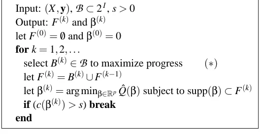
_{. Mathematically this requirement} is non-important because we may simply assign∞coding length to single-element blocks, which is equivalent to excluding these single element sets.

Input:(X,y),

B

_⊂2I_{, s>0} Output: F(k)andβ(k) let F(0)=/0andβ(0)=0 for k=1,2, . . .

select B(k)∈

B

_{to maximize progress (∗)} let F(k)=B(k)∪F(k−1)

letβ(k)=arg min_β∈RpQˆ(β)subject to supp(β)⊂F(k) if (c(β(k)_{)>s) break}

end

Figure 1: Structured Greedy Algorithm

In Figure 1, we are given a set of blocks

B

_{that contains subsets of}

I

_{. Instead of searching all} subsets F_⊂

I

_{up to a certain complexity|F|+c(F), which is computationally infeasible, we search} only the blocks restricted to

B

_{. It is assumed that searching over}

B

_{is computationally manageable.} In practice, the computational cost is linear in the number of base blocks_|

B

_|.

At each step(_∗), we try to find a block from

B

_{to maximize progress. It is thus necessary to} define a quantity that measures progress. Our idea is to approximately maximize the gain ratio:

ˆ

Q(β(k₋1)_)−Qˆ(β(k)₎ c(β(k)_)−c(βk−1₎ ,

which measures the reduction of objective function per unit increase of coding complexity. This greedy criterion is a natural generalization of the standard greedy algorithm, and essential in our analysis. For least squares regression, we can define the gain ratio as follows:

φ(B) =kPB−F(k−1)(Xβ

(k−1)_−y)k2 2

c(B_∪F(k−1)_)−c(F(k−1)₎, (5)

where

PF =XF(XF⊤XF)+XF⊤

is the projection matrix to the subspaces generated by columns of XF. Here(XF⊤XF)+denotes the

More precisely, for least squares regression, at each step(_∗)of Figure 1, we select a block B(k) that satisfies the condition

φ(B(k))_≥νmax

B∈Bφ(B) (6)

for some ν_∈(0,1]. We may regard ν as a fixed approximation ratio (to ensure the quality of approximate optimization) that will appear in our analysis, although the algorithm does not have to pickνa priori.

The reason to allow approximate maximization in (6) is that our practical implementation of StructOMP maximizes a simpler quantity

˜

φ(B) =kX ⊤

B−F(k−1)(Xβ(k−1)−y)k22

c(B∪F(k−1)_)−c(F(k−1)₎, (7)

which is more efficient to compute (especially when blocks are overlapping). Since the ratio

kX_B⊤_−F(k−1)rk22/kPB₋F(k−1)rk2₂

is bounded betweenρ+(B)andρ₋(B) (these quantities are defined in Definition 4), we know that maximization of ˜φ(B)leads to an approximate maximization ofφ(B)withν≥ρ−(B)/ρ+(B). That is, maximization of (7) in our practical StructOMP implementation corresponds to an approximate maximization in (6). Moreover,νonly appears in our analysis, and it does not appear explicitly in our implementation.

Note that we shall ignore B_∈

B

_{such that B⊂F}(k−1)_{, and just let the corresponding gain to be} 0. Moreover, if there exists a base block B_6⊂F(k−1)but c(B_∪F(k−1))_≤c(F(k−1)), we can always select B and let F(k)=B∪F(k−1)(this is because it is always beneficial to add more features into

F(k) without additional coding complexity). We assume this step is always performed if such a

B_∈

B

_{exists. The non-trivial case is c(B∪F}(k−1)_)>c(F(k−1)_{)for all B∈}

B

_{; in this case both}φ_(B) and ˜φ(B)are well defined.

3.2 Convergence Analysis

It is important to understand that the block structure is only used to limit the search space in the structured greedy algorithm. However, our theoretical analysis shows that if in addition, the un-derlying coding scheme can be approximated by block coding using base blocks employed in the greedy algorithm, then the algorithm is effective in minimizing (2). Although one does not need to know the specific approximation in order to use the greedy algorithm, knowing its existence (which can be shown for the examples discussed in Section 4) guarantees the effectiveness of the algorithm. It is also useful to understand that our result does not imply that the algorithm won’t be effective if the actual coding scheme cannot be approximated by block coding.

We shall introduce a definition before stating our main results.

Definition 8 Given

B

_⊂2I_{, define}

ρ0(

B

) =max

B_∈Bρ+(B), c0(

B

_{) =max}

B_∈Bc(B)

and

c(β¯,

B

_{) =min}

( b

∑

j=1

c(_B¯_{j): supp(β}¯_)⊂[b

j=1 ¯

Bj (B¯j∈

B

); b≥1 )

The following theorem shows that if c(β¯,

B

_{)is small, then one can use the structured greedy} algo-rithm to find a coefficient vectorβ(k)that is competitive to ¯β, and the coding complexity c(β(k)_)is

not much worse than that of c(β¯,

B

_{). This implies that if the original coding complexity c(}β¯_{)can be} approximated by block complexity c(β¯,

B

_{), then we can approximately solve (2).}

Theorem 9 Suppose the coding scheme is sub-additive. Consider ¯βandεsuch that

ε∈(0,_ky_k22_{− k}X ¯β₋y_k2₂]

and

s_≥ ρ0(

B

)c(

¯

β,

B

₎

νρ₋(s+c(β¯))ln

ky_k2_{2− k}X ¯β₋y_k2₂

ε .

Then at the stopping time k, we have

ˆ

Q(β(k))_≤Qˆ(β¯) +ε.

By Theorem 6, the result in Theorem 9 implies that

kXβ(k)₋Ey_k2≤ kX ¯β−Eyk2+σ

p

2 ln(6/η) +2σ

q

7.4(s+c0(

B

)) +4.7 ln(6/η) +ε/σ2,

kβ(k)−β¯k22≤

10_kX ¯β₋Ey_k2₂+37σ2(s+c0(

B

)) +29σ2ln(6/η) +2.5ε

ρ₋(s+c0(

B

) +c(β¯))n

.

The result shows that in order to approximate a signal ¯β up to accuracy ε, one needs to use coding complexity O(ln(1/ε))c(β¯,

B

_{). Now, consider the case that}

B

_{contains small blocks and} their sub-blocks with equal coding length, and the actual coding scheme can be approximated (up to a constant) by block coding generated by

B

_{; that is, c(}β¯_,

B

_{) =O(c(}β¯_{)). In this case we need}

O(s ln(1/ε))to approximate a signal with coding complexity s. For this reason, we will extensively discuss block approximation in Section 4.

In order to improve forward greedy procedures, backward greedy strategies can be employed, as shown in various recent works such as Zhang (2011). For simplicity, we will not analyze such strategies in this paper. It is worth mentioning that in practice, greedy algorithm is often adequate. In particular the O(ln(1/ε))factor vanishes for a weakly sparse target signal ¯β, where the magnitude of its coefficients gradually decrease to zero. This concept has been considered in previous work such as Donoho (2006) and Baraniuk et al. (2010). In such case, we may choose an appropriate optimal stopping point to avoid the O(ln(1/ε))factor. In fact, practitioners often observe that OMP can be more effective than Lasso for weakly sparse target signals (in spite of stronger theoretical results for Lasso with strongly sparse target signals). This will be confirmed in our experiments as well. Without cluttering the main text, we leave the detailed analysis of StructOMP for weakly sparse signals to Appendix F. Our analysis is the first theoretical justification of this empirical phenomenon.

4. Structured Sparsity Examples

a small number of base blocks (a block is a subset of

I

_{), and then define a coding scheme on all} subsets of

I

_{using these base blocks.}

Consider block set

B

_⊂2I_{. We assume that every subset F ⊂}

I

_{can be expressed as the union} of blocks in

B

_{. Let cl0be a code length on}

B

_:

∑

B_∈B

2−cl0(B)_≤1,

we define cl(B) =cl0(B) +1 for B∈

B

. It not difficult to show that the following cost function on

F_⊂

I

_{is a coding length}

clB(F) =min (

b

∑

j=1

cl(Bj): F= b

[

j=1

Bj (Bj∈

B

) )

.

This is because

∑

F⊂I_,F6=/0

2−cl(F)_≤

∑

b≥1Bℓ∈B

∑

_:1≤ℓ≤b

2−∑bℓ=1cl(Bℓ)≤

∑

b≥1

b

∏

ℓ=1B

∑

ℓ∈B

2−cl(Bℓ)_≤

∑

b≥1

2−b=1.

We call the coding scheme clB block coding. It is clear from the definition that block coding is

sub-additive.

From Theorem 9 and the discussions thereafter, we know that under appropriate conditions, a target coefficient vector with a small block coding complexity can be approximately learned using the structured greedy algorithm. This means that the block coding scheme has important algorithmic implications. That is, if a coding scheme can be approximated by block coding with a small number of base blocks, then the corresponding estimation problem can be approximately solved using the structured greedy algorithm.

For this reason, we shall pay special attention to block coding approximation schemes for ex-amples discussed below. In particular, a coding scheme cl(_·) can be polynomially approximated by block coding if there exists a block coding scheme clB with polynomial (in p) number of base

blocks in

B

_{, such that there exists a positive constant CB independent of p:}

clB(F)≤CBcl(F).

That is, up to a constant, the block coding scheme clB()is dominated by the coding scheme cl().

While it is possible to work with blocks with non-uniform coding schemes, for simplicity ex-amples provided in this paper only consider blocks with uniform coding, which is similar to the representation used in the Union-of-Subspaces model of Lu and Do (2008).

4.1 Standard Sparsity

A simple coding scheme is to code each subset F _⊂

I

_{of cardinality k using k log}

2(2p)bits, which corresponds to block coding with

B

_{consisted only of single element sets, and each base block has} a coding length cl0=log2p. This corresponds to the complexity for the standard sparse learning.

A more general version is to consider single element blocks

B

_{={{j}: j∈}

I

_{}, with a} non-uniform coding scheme cl0({j}) =cj, such that ∑j2−cj ≤1. It leads to a non-uniform coding

length on

I

_as

cl(B) =_|B_|+

∑

In particular, if a feature j is likely to be nonzero, we should give it a smaller coding length cj, and

if a feature j is likely to be zero, we should give it a larger coding length. In this case, a subset

F_⊂

I

_{has coding length cl(F) =}∑

j∈F(1+cj).

4.2 Group Sparsity

The concept of group sparsity has appeared in various recent work, such as the group Lasso in Yuan and Lin (2006) or multi-task learning in Argyriou et al. (2008). Consider a partition of

I

_=∪m

j=1Gj

into m disjoint groups. Let

B

_{Gcontain the m groups{Gj}, and}

B

_{1contain p single element blocks.} The strong group sparsity coding scheme is to give each element in

B

_{1 a code-length cl0 of}∞_, and each element in

B

_{G a code-length cl0 of log}

2m. Then the block coding scheme with blocks

B

₌

B

_G∪

B

_{1 leads to group sparsity, which only looks for signals consisted of the groups. The} resulting coding length is: cl(B) =g log₂(2m) if B can be represented as the union of g disjoint groups Gj; and cl(B) =∞otherwise.

Note that if the support of the target signal F can be expressed as the union of g groups, and each group size is k0, then the group coding length g log₂(2m)can be significantly smaller than the standard sparsity coding length of_|F_|log₂(2p) =gk0log2(2p). As we shall see later, the smaller coding complexity implies better learning behavior, which is essentially the advantage of using group sparse structure. It was shown by Huang and Zhang (2010) that strong group sparsity defined above also characterizes the performance of group Lasso. Therefore if a signal has a pre-determined group structure, then group Lasso is superior to the standard Lasso.

An extension of this idea is to allow more general block coding length for cl0(Gj)and cl0({j}) so that

m

∑

j=1

2−cl0(Gj)₊

p

∑

j=1

2−cl0({j})_≤1.

This leads to non-uniform coding of the groups, so that a group that is more likely to be nonzero is given a smaller coding length. If feature set F can be represented as the union of g groups

Gj1, . . . ,Gjg, then its coding length is cl(F) =g+∑

g

j=1cl0(Gj).

Figure 2: Group sparsity: nodes are variables, and black nodes are selected variables

Group sparsity is a special case of graph sparsity discussed below. Figure 2 shows an example of group sparsity, where the variables are represented by nodes, and the selected variables are rep-resented by black nodes. Each pre-defined group is reprep-resented as a connected components in the graph, and the example contains six groups. Two groups, the first and the third from the left, are se-lected in the example. The number of sese-lected variables (black nodes) is seven. Therefore we have

4.3 Hierarchical Sparsity

One may also create a hierarchical group structure. A simple example is wavelet coefficients of a signal (Mallat, 1999). Another simple example is a binary tree with the variables as leaves, which we describe below. Each internal node in the tree is associated with three options: only left child, only right child, or both children; each option can be encoded in log₂3 bits.

Given a subset F _⊂

I

_{, we can go down from the root of the tree, and at each node, decide} whether only left child contains elements of F, or only right child contains elements of F, or both children contain elements of F. Therefore the coding length of F is log₂3 times the total number of internal nodes leading to elements of F. Since each leaf corresponds to no more than log₂p

internal nodes, the total coding length is no worse than log₂3 log₂p_|F_|. However, the coding length can be significantly smaller if nodes are close to each other or are clustered. In the extreme case, when the nodes are consecutive, we have O(_|F_|+log₂p) coding length. More generally, if we can order elements in F as F =_{j1, . . . ,jq}, then the coding length can be bounded as cl(F) = O(_|F|+log₂p+∑q_s=2log₂minℓ<s|js−jℓ|).

If all internal nodes of the tree are also variables in

I

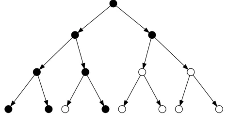
_{(for example, in the case of wavelet} decomposition), then one may consider feature set F with the following property: if a node is selected, then its parent is also selected. This requirement is very effective in wavelet compression, and often referred to as the zero-tree structure (Shapiro, 1993). Similar requirements have also been applied in statistics (Zhao et al., 2009) for variable selection and in compressive sensing (Baraniuk et al., 2010). The argument presented in this section shows that if we require F to satisfy the zero-tree structure, then its coding length is at most O(_|F_|), without any explicit dependency on the dimensionality p. This is because one does not have to reach a leave node. Figure 3 shows an example of hierarchical sparsity, where the nodes of the tree are variables, and black nodes indicate those variables that are selected. The total number of selected variables (number of black nodes) is_|F_|=8. This example obeys the requirement that if a node is selected, then its parent is also selected. Therefore the complexity is measured by O(_|F|).

Figure 3: Hierarchical sparsity: nodes are variables, and black nodes are selected variables

4.4 Graph Sparsity

We consider a generalization of the hierarchical and group sparsity ideas by employing a (directed or undirected) graph structure G on

I

_{. To the best of our knowledge, this general structure has not} been considered in any previous work.

In graph sparsity, each variable (an element of

I

_{) is a node of G but G may also contain} ad-ditional nodes that are not variables. In order to take advantage of the graph structure, we favor connected regions (that is, nodes that are grouped together with respect to the graph structure). The following result defines a coding length on graphs based on the underlying graph structure. We leave its analysis to Appendix A.

Proposition 10 Let G be a graph with maximum degree dG. There exists a constant CG≤2 log2(1+

dG)such that for any probability distribution q on G (∑v_∈Gq(v) =1 and q(v)≥0 for v∈G), the following quantity (which we call graph coding) is a coding length on 2G:

cl(F) =CG|F|+g− g

∑

j=1 max

v∈Fj

log₂(q(v)),

where F_⊂2Gcan be decomposed into the union of g connected components F =_∪g_j=1Fj.

Note that graph coding is sub-additive. As a concrete example, we consider image processing, where each image is a rectangle of pixels (nodes); each pixel is connected to four adjacent pixels, which forms the underlying graph structure. We may take q(v) =1/p for all v_∈G, where p=_|G_|

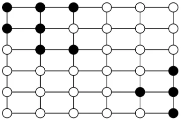
is the number of variables. Proposition 10 implies that if F is composed of g connected regions, then the coding length is g log₂(2p) +2 log₂(5)_|F_|, which can be significantly better than standard sparse coding length of|F|log₂(2p). For example, Figure 4 shows an image grid, where nodes are variables and selected variables are denoted by black nodes. In this example, the selected variables have two connected components (that is, g=2): one in the top-left part, and the other in the bottom-right part of the grid. The total number of selected variables (the number of black nodes) is|F|=11.

Figure 4: Graph sparsity: nodes are variables, and black nodes are selected variables

not need to know the specific group divisions a priori as in Figure 2. From Proposition 10, similar coding complexity can be obtained as long as F can be covered by a small number of connected regions. Tree-structured hierarchical sparsity is also a special case of graph sparsity with a single connected region containing the root (we may take q(root) =1). In fact, one may generalize this concept as follows. We consider a special case of sparse sparsity where we limit F to be a connected region that contains a fixed starting node v0. We can simply let q(v0) =1, and the coding length of

F is O(_|F_|), which is independent of the dimensionality p. This generalizes the similar claim for the zero-tree structure described earlier.

Figure 5: Line-structured sparsity: nodes are variables, and black nodes are selected variables

The following result shows that under uniform encoding of the nodes q(v) =1/p for v_∈G,

general graph coding schemes can be polynomially approximated with block coding. The idea is to consider relatively small sized base blocks consisted of nodes that are close together with respect to the graph structure, and then use the induced block coding scheme to approximate the graph coding.

Proposition 11 Let G be a graph with maximum degree dG, and p=|G|. Consider any numberδ>

0 such that L=δlog₂p is an even integer. Let

B

_{be the set of connected nodes of size up to L; that is,}

B_∈

B

_{is a connected region in G such that|B| ≤L. Then there exists a constant CG≤2 log}

2(1+dG), such that _|

B

_{| ≤p}1+CGδ_{. If we consider the uniform code-length cl}

0(B) = (1+CGδ)log2p for all

B_∈

B

_{, then the induced block-coding scheme clB satisfies}

clB(F)≤g(1+C_Gδ)log₂p+2(C_G+δ−1)|F|. where g is the number of connected regions in F.

The result means that graph sparsity can be polynomially approximated with a block coding scheme if we let q(v) =1/p for all v_∈G. As we have pointed out, block approximation is useful

because the latter is required in the structured greedy algorithm which we propose in this paper. Note that a refined result holds for hierarchical sparsity (where we have q(root) =1) using block approximation that does not explicitly depend on log₂p. In this case, for each tree depth

ℓ=1,2,3, . . ., we can restrict the underlying tree upto depth ℓ, and apply Proposition 11 on the

restricted tree. Using this idea, the coding length for F depends explicitly on the maximum depth of F in the tree instead of log₂p.

4.5 Random Field Sparsity

Let zj∈ {0,1}be a random variable for j∈

I

that indicates whether j is selected or not. The most

general coding scheme is to consider a joint probability distribution of z= [z1, . . . ,zp]. The coding

length for F can be defined as₋log₂p(z1, . . . ,zp)with zj =I(j∈F)indicating whether j∈F or

not.

should take 1 with probability close to O(1/p), so that the expected number of j’s with zj =1

is O(1). For disconnected graphs (zj are independent), the variables zj are iid Bernoulli random

variables with probability 1/p being one. In this case, the coding length of a set F is_|F_|log₂(p)₋ (p− |F|)log₂(1−1/p)_{≈ |}F|log₂(p) +1. This is essentially the probability model for the standard sparsity scheme. In a more sophisticated situation, one may also let E(zj)to grow with sample size n. This is useful in non-parametric statistics.

We note that random field model has been considered in Cevher et al. (2009a). For many such models, it is possible to approximate a general random field coding scheme with block coding by using approximation methods in the graphical model literature. However, such approximations are problem specific, and the details are beyond the scope of this paper.

5. Experiments

The purpose of these experiments is to demonstrate the advantage of structured sparsity over stan-dard sparsity. We compare the proposed StructOMP to OMP and Lasso, which are stanstan-dard algo-rithms to achieve sparsity but without considering structure (Tibshirani, 1996; Tropp and Gilbert, 2007). For graph sparsity, the choice of c(F)is simply c(F) =g log₂p+_|F_|, where g is the number of connected regions of F. This is adequate based on the discussion in Section 3. However, as pointed out after Definition 1, a better method is to use c(F) =g log₂p+γ_|F_|, where we tuneγ appropriately. We observe that in practice, such tuning often improves performance. Nevertheless, in our experiments, we only report results with fixedγ=1 for simplicity. This also means our ex-periments only demonstrate the advantage of StructOMP very conservatively without fine-tuning. The base blocks used in StructOMP are described in each experiment. Parameters (such as s in StructOMP orλin Lasso) are tuned by cross-validation on the training data. We test various aspects of our theory to check whether the experimental results are consistent with the theory. Although in order to fully test the theory, one should also verify the RIP (or structured RIP) assumptions, in practice this is difficult to check precisely (however, it is possible to verify it approximately using ideas of d’Aspremont et al., 2008). Therefore in the following, we shall only study whether the ex-perimental results are consistent with what can be expected from our theory, without verifying the detailed assumptions. The experimental protocols follow the setup of compressive sensing, where the original signals are projected using random projections, with noise added. Our goal is to recover the original signals from the noise corrupted projections.

In the experiments, we use Lasso-modified least angle regression (LARS/Lasso) as the solver of Lasso (B. Efron and Tibshirani, 2004). In order to quantitatively compare performance of different algorithms, we use recovery error, defined as the relative difference in 2-norm between the estimated sparse coefficient vector ˆβest and the ground-truth sparse coefficient ¯β: kβˆest−β¯k2/kβ¯k2. Our experiments focus on graph sparsity, with several different underlying graph structures. Note that graph sparsity is more general than group sparsity; in fact connected regions may be regarded as dynamic groups that are not pre-defined. However, for illustration, we include a comparison with group Lasso using some 1D simulated examples, where the underlying structure can be more easily approximated by pre-defined groups. Since additional experiments involving more complicated structures are more difficult to approximate by pre-defined groups, we exclude group-Lasso in those experiments.

simulation experiments, we use k to denote the sparsity (number of nonzeros) of the true signal, and this should not be confused with the number of iterations k which we used earlier in the description of the StructOMP algorithm.

5.1 Simulated 1D Signals with Line-Structured Sparsity

In the first experiment, we randomly generate a 1D structured sparse signal with values_±1, where data dimension p=512, sparsity number k=64 and group number g=4. The support set of these signals is composed of g connected regions. Here, each component of the sparse coefficient is connected to two of its adjacent components, which forms the underlying graph structure. The graph sparsity concept introduced earlier is used to compute the coding length of sparsity patterns in StructOMP. The projection matrix X is generated by creating an n_×p matrix with i.i.d. draws

from a standard Gaussian distribution N(0,1). For simplicity, the rows of X are normalized to unit magnitude. Zero-mean Gaussian noise with standard deviationσ=0.01 is added to the measure-ments. Our task is to compare the recovery performance of StructOMP to those of OMP, Lasso and group Lasso for these structured sparsity signals under the framework of compressive sensing.

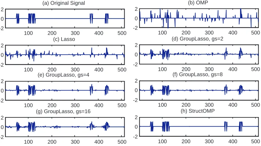
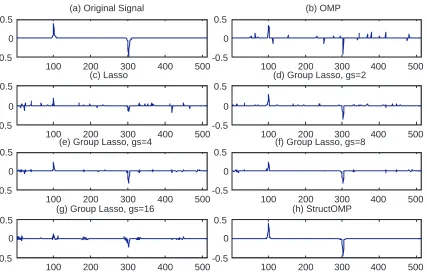
Figure 6 shows one instance of generated signal and the corresponding recovered results by different algorithms when n=160. Since the sample size n is not big enough, OMP and Lasso do not achieve good recovery results, whereas the StructOMP algorithm achieves near perfect recovery of the original signal. We also include group Lasso in this experiment for illustration. We use predefined consecutive groups that do not completely overlap with the support of the signal. Since we do not know the correct group size, we just try group Lasso with several different group sizes (gs=2, 4, 8, 16). Although the results obtained with group Lasso are better than those of OMP and Lasso, they are still inferior to the results with StructOMP. As mentioned, this is because the pre-defined groups do not completely overlap with the support of the signal, which reduces the efficiency. In StructOMP, the base blocks are simply small connected line segments of size gs=3: that is, one node plus its two neighbors. This choice is only for simplicity, and it already produces good results in our experiments. If we include larger line segments into the base blocks (e.g., segments of size gs=4,5, etc), one can expect even better performance from StructOMP.

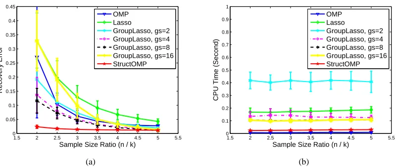
To study how the sample size n effects the recovery performance, we vary the sample size and record the recovery results by different algorithms. To reduce the randomness, we perform the experiment 100 times for each sample size. Figure 7(a) shows the recovery performance in terms of Recovery Error and Sample Size, averaged over 100 random runs for each sample size. As expected, StructOMP is better than the group Lasso and far better than the OMP and Lasso. The results show that the proposed StructOMP can achieve better recovery performance for structured sparsity signals with less samples. Figure 7(b) shows the recovery performance in terms of CPU Time and Sample Size, averaged over 100 random runs for each sample size. The computation complexities of StructOMP and OMP are far lower than those of Lasso and Group Lasso.

RIP condition is easier to satisfied for weakly sparse signals (based on our theory). Therefore the experimental results are consistent with our theory.

100 200 300 400 500

-2 0 2

(a) Original Signal

100 200 300 400 500

-2 0 2

(c) Lasso

100 200 300 400 500

-2 0 2

(e) GroupLasso, gs=4

100 200 300 400 500

-2 0 2

(g) GroupLasso, gs=16

100 200 300 400 500

-2 0 2

(b) OMP

100 200 300 400 500

-2 0 2

(d) GroupLasso, gs=2

100 200 300 400 500

-2 0 2

(f) GroupLasso, gs=8

100 200 300 400 500

-2 0 2

(h) StructOMP

Figure 6: Recovery results of 1D signal with strongly line-structured sparsity. (a) original data; (b) recovered results with OMP (error is 0.9921); (c) recovered results with Lasso (er-ror is 0.8660);; (d) recovered results with Group Lasso (er(er-ror is 0.4832 with group size gs=2); (e) recovered results with Group Lasso (error is 0.4832 with group size gs=4);(f) recovered results with Group Lasso (error is 0.2646 with group size gs=8);(g) recovered results with Group Lasso (error is 0.3980 with group size gs=16); (h) recovered results with StructOMP (error is 0.0246).

To study how the additive noise affects the recovery performance, we adjust the noise powerσ and then record the recovery results by different algorithms. In this case, we fix the sample size at

n=3k=192, and perform the experiment 100 times for each noise level tested. Figure 8(a) shows the recovery performance in terms of Recovery Error and Noise Level, averaged over 100 random runs for each noise level. As expected, StructOMP is also better than the group Lasso and far better than the OMP and Lasso. Figure 8(b) shows the recovery performance in terms of CPU Time and Noise Level, averaged over 100 random runs for each sample size. The computational complexities of StructOMP and OMP are lower than those of Lasso and Group Lasso.

1.5 2 2.5 3 3.5 4 4.5 5 5.5 0 0.2 0.4 0.6 0.8 1 1.2 1.4 1.6 Recovery Error

Sample Size Ratio (n / k) OMP Lasso GroupLasso, gs=2 GroupLasso, gs=4 GroupLasso, gs=8 GroupLasso, gs=16 StructOMP (a)

1.5 2 2.5 3 3.5 4 4.5 5 5.5

0 0.05 0.1 0.15 0.2 0.25 0.3 0.35 0.4 0.45 0.5 Time

Sample Size Ratio (n / k) OMP Lasso GroupLasso, gs=2 GroupLasso, gs=4 GroupLasso, gs=8 GroupLasso, gs=16 StructOMP (b)

Figure 7: Recovery performance: (a) Recovery Error vs. Sample Size Ratio(n/k); (b) CPU Time vs. Sample Size Ratio(n/k)

0 0.05 0.1 0.15 0.2

0 0.5 1 1.5 2 Recovery Error

Noise Level (sigma) OMP Lasso GroupLasso, gs=2 GroupLasso, gs=4 GroupLasso, gs=8 GroupLasso, gs=16 StructOMP (a)

0 0.05 0.1 0.15 0.2

0 0.05 0.1 0.15 0.2 0.25 0.3 0.35 0.4 0.45 0.5 Time

Noise Level (sigma) OMP Lasso GroupLasso, gs=2 GroupLasso, gs=4 GroupLasso, gs=8 GroupLasso, gs=16 StructOMP (b)

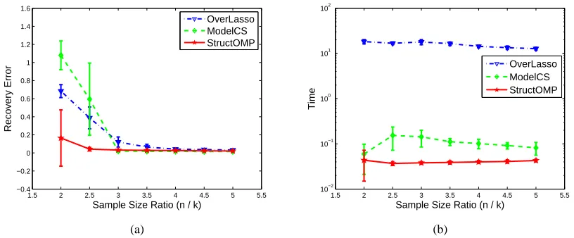
performance in terms of Recovery Error and Sample Size, averaged over 100 random runs for each sample size. At least for this problem, StructOMP achieves better performance than OverlapLasso and ModelCS, which shows that the proposed StructOMP algorithm can achieve better recovery performance than other structured sparsity algorithms for some problems. Figure 9(b) shows the recovery performance in terms of CPU Time and Sample Size, averaged over 100 random runs for each sample size. Although it is difficult to see from the figure, the computational complexity of StructOMP is lower than that of ModelCS (about half CPU time) and are far lower than that of OverlapLasso, at least based on the implementation of Jacob et al. (2009).

1.5 2 2.5 3 3.5 4 4.5 5 5.5

−0.4 −0.2 0 0.2 0.4 0.6 0.8 1 1.2 1.4 1.6

Recovery Error

Sample Size Ratio (n / k)

OverLasso ModelCS StructOMP

(a)

1.5 2 2.5 3 3.5 4 4.5 5 5.5

10−2 10−1 100

101 102

Time

Sample Size Ratio (n / k)

OverLasso ModelCS StructOMP

(b)

Figure 9: Performance Comparisons between methods related with structured

spar-sity(OverlapLasso (Jacob et al., 2009), ModelCS (Baraniuk et al., 2010), StructOMP): (a) Recovery Error vs. Sample Size Ratio(n/k); (b) CPU Time vs. Sample Size Ratio

(n/k)

Note that Lasso performs better than OMP in the first example. This is because the signal is strongly sparse (that is, all nonzero coefficients are significantly different from zero). In the second experiment, we randomly generate a 1D structured sparse signal with weak sparsity, where the nonzero coefficients decay gradually to zero, but there is no clear cutoff. One instance of generated signal is shown in Figure 10 (a). Here, p=512 and all coefficient of the signal are not zeros. We define the sparsity k as the number of coefficients that contain 95% of the image energy. The support set of these signals is composed of g=2 connected regions. Again, each element of the sparse coefficient is connected to two of its adjacent elements, which forms the underlying 1D line graph structure. The graph sparsity concept introduced earlier is used to compute the coding length of sparsity patterns in StructOMP. The projection matrix X is generated by creating an n_×p matrix

with i.i.d. draws from a standard Gaussian distribution N(0,1). For simplicity, the rows of X are normalized to unit magnitude. Zero-mean Gaussian noise with standard deviationσ=0.01 is added to the measurements.

Figure 10 shows one generated signal and its recovered results by different algorithms when

group sizes (gs=2, 4, 8, 16). Although the results obtained with group Lasso are better than those of OMP and Lasso, they are still inferior to the results with StructOMP. In order to study how the sample size n effects the recovery performance, we vary the sample size and record the recovery results by different algorithms. To reduce the randomness, we perform the experiment 100 times for each of the sample sizes.

Figure 11(a) shows the recovery performance in terms of Recovery Error and Sample Size, averaged over 100 random runs for each sample size. As expected, StructOMP algorithm is superior in all cases. What’s different from the first experiment is that the recovery error of OMP becomes smaller than that of Lasso. This result is consistent with our theory, which predicts that if the underlying signal is weakly sparse, then the relatively performance of OMP becomes comparable to Lasso. Figure 11(b) shows the recovery performance in terms of CPU Time and Sample Size, averaged over 100 random runs for each sample size. The computational complexities of StructOMP and OMP are far lower than those of Lasso and Group Lasso.

100 200 300 400 500

-0.5 0 0.5

(a) Original Signal

100 200 300 400 500

-0.5 0 0.5

(c) Lasso

100 200 300 400 500

-0.5 0 0.5

(e) Group Lasso, gs=4

100 200 300 400 500

-0.5 0 0.5

(g) Group Lasso, gs=16

100 200 300 400 500

-0.5 0 0.5

(b) OMP

100 200 300 400 500

-0.5 0 0.5

(d) Group Lasso, gs=2

100 200 300 400 500

-0.5 0 0.5

(f) Group Lasso, gs=8

100 200 300 400 500

-0.5 0 0.5

(h) StructOMP