Multiple-Instance Learning of Real-Valued Data
Daniel R. Dooly [email protected]
Department of Computer Science Southern Illinois University Edwardsville Edwardsville, IL 62026-1656, USA
Qi Zhang [email protected]
Sally A. Goldman [email protected]
Department of Computer Science and Engineering Washington University
St. Louis, MO 63130-4899, USA
Robert A. Amar [email protected]
Georgia Institute of Technology College of Computing
801 Atlantic Drive
Atlanta, GA 30332-0280, USA
Editors: Carla E. Brodley and Andrea Danyluk
Abstract
The multiple-instance learning model has received much attention recently with a primary ap-plication area being that of drug activity prediction. Most prior work on multiple-instance learning has been for concept learning, yet for drug activity prediction, the label is a real-valued affinity measurement giving the binding strength. We present extensions of k-nearest neighbors (k-NN), Citation-kNN, and the diverse density algorithm for the real-valued setting and study their per-formance on Boolean and real-valued data. We also provide a method for generating chemically realistic artificial data.
1. Introduction
The multiple-instance learning model is becoming increasingly important within machine learning. Unlike standard supervised learning in which each instance is labeled in the training data, in this model each example is a set (or bag)1of instances which is labeled as to whether any single instance within the bag is positive. The individual instances are not given a label. The goal of the learner is to generate a hypothesis to accurately predict the label of previously unseen bags. Consider the standard learning problem of learning an axis-aligned box inℜn. In the standard learning model each labeled example is a point in ℜn (drawn according to some unknown distribution
D
) and labeled as positive if and only if it is in the target box. In the multi-instance model, an example is a collection of points inℜn(often called a bag or r-example) which is labeled as positive if and only if at least one of the points in the bag is in the target box.The multiple-instance model was motivated by the drug activity prediction problem where each example is a possible configuration (or shape) for a molecule of interest and each bag contains all low-energy (and hence likely) configurations for the molecule (Dietterich, T. G., Lathrop, R. H. and Lozano-P´erez, T, 1997). For the drug discovery application, each bag corresponds to a drug, each point in the bag corresponds to the shapes that it is likely to take, and the target point corresponds to the ideal shape that will create the strongest bind with the receptor molecule. By accurately pre-dicting which molecules will bind to an unknown protein, one can accelerate the discovery process for new drugs, hence reducing cost.
The algorithms we present here are quite general. We assume that each bag in the training data,
B
, contains a set of any number of instances where each instance is described by a set of n features. Thus, we can view this problem as a geometric learning problem where each bag is a set of any number of n-dimensional points. For the drug activity prediction problem typically one would expect one point in the bag for each low-energy conformation. The inductive bias upon which our algorithms depend is that there is some unknown target point (in the n-dimensional feature space) and the label of a point pi,jis a non-increasing function of the distance between the target point andpi,junder some unknown metric. The label of the bag is based on the point in the bag closest to the
target point. Any representation of a molecule as a set of n-dimensional points that shares this bias would be applicable when applying our algorithm.
In the standard multiple-instance model with Boolean labels, any bag containing only points sufficiently distant from the target will be labeled negative and the others will be labeled as pos-itive. More formally, let
B
=. {hB1,`1i,hB2,`2i,...hB|B|,`|B|i} where `i is the label of bag Bi.Bi=. {pi,1,pi,2,...pi,|Bi|}, and`i,j is the label of point pi,j ∈Bi. Then∀i`i
.
=`i,1∨`i,2∨...∨`i,|Bi|.
In standard supervised learning, we can see the label of each point. In the multiple-instance model we can see only the labels of the bags.
{hp1,1,`1,1i,...hp1,|B1|,`1,|B1|i
| {z }, hp2,1,`2,1i,...hp2,|B2|,`2,|B2|i
| {z }, ... }
{hB1,`1i, hB2,`2i, ... }
There has been a significant amount of research directed towards this problem (Auer 1997; Maron and Lozano-P`erez, 1998, Maron 1998, Wang and Zucker 2000). Other applications for the multiple-instance model have also been proposed (Maron and Raton, 1998; Ruffo 2000). For example, Maron and Raton (1998) applied the multiple-instance model to the task of learning to recognize a person from a series of images that are labeled positive if they contain the person and negative otherwise. They have also applied this model to learn descriptions of natural images (such as a waterfall) and then used the learned concept to retrieve similar images from a large image database. More recently, Ruffo (2000) has used this model for data mining applications.
Most prior research performed under the multiple-instance model is for concept learning (i.e. Boolean labels). The first empirical study of Dietterich et al. (1997) used real data for the problem of predicting whether or not a synthetic molecule binds to the musk receptor. However, binding affinity between molecules and receptors is quantitative, borne out in quantities such as the energy released by the molecule-receptor pair upon binding (the more energy, the better the bond) and hence a real-valued classification of binding strength in these situations is preferable to a binary classification.
strength of a drug is a major factor in its economy and toxicological effects on patients; strongly binding drugs need to be produced in lower quantities, and lower doses may represent a benefit to the patients using the drugs. Hence, in real drug-discovery work, most data is labeled with real-valued affinity measurements obtained via laboratory work. The only real data sets available as benchmarks are the Musk1 and Musk2 data sets provided by Dietterich et al. (1997) for the problem of predicting the strength of synthetic musk molecules. Presumably, positive examples of musk molecules bind well to olfactory receptors and negative examples do not. However, the key question is often not whether or not a molecule binds, but how strong the tendency to bind is. Dietterich et al. note that “The only aspect of the musk problem that is substantially different from typical pharmaceutical problems is that the musk strength is measured qualitatively by expert human judges, whereas drug activity binding is usually measured quantitatively through biochemical assays.” We argue later that other aspects of the musk data sets are also atypical.
In this paper, we study extensions of the diversity density, k-NN, and citation-kNN algorithms for the real-valued multiple-instance setting. We look at both the squared loss and the prediction error (where all labels> .5 are treated as 1 and the rest are treated as 0).2 While our paper focuses on studying the real-valued multiple-instance setting, we also want to deepen our understanding of algorithms that have been proposed for the Boolean setting. Despite some criticism of the musk data sets, most notably by Maron (1998) in regards to the MULTINST algorithm working well despite the strong (and inaccurate) distributional assumptions it makes, these data sets are still widely used as experimental benchmarks for multiple-instance learners. Along with some real-valued benchmarks, additional Boolean benchmarks are needed. Wang and Zucker (2000) note that, “Although the two adaptation algorithms of k-NN performed remarkably well, the basic reasons why they acquired such high accuracy on the musk data sets are unclear.” The ability to generate artificial data sets has enabled us to answer this question and others like it.
We provide two baselines with which to compare our work. In the first baseline, a random bag from the training data is selected and its label is returned. As a second baseline, we use the standard unweighted k-NN algorithm by converting the multiple-instance problem to a standard supervised learning problem by assigning each point the label of its bag. Then, the standard (single-instance) k-NN algorithm using the Euclidean distance is used. We compare the performance of these algo-rithms when using real-valued data to their performance when using Boolean labels obtained by rounding the real-valued labels to 0 or 1. Even when the training data has only labels of 0 or 1, the prediction is real-valued. For example, for k-NN, the average label from the k-nearest neighbors is output. We report the squared loss between the underlying real-valued label and the real-valued prediction made by the algorithm that received only Boolean labels. Not surprisingly, we found the squared-loss is greatly reduced when using real-valued labels versus the Boolean labels obtained by rounding.
Our empirical work has provided some valuable new insights about these algorithms. A sec-ondary contribution of our work is a procedure for generating chemically realistic artificial data in which you can control factors such as the number of conformers, the number of relevant features, and their degree of relevance. We have placed the data sets used in this paper at
www.cs.wustl.edu/∼sg/multi-inst-data/.
2. Previous Work
In their seminal paper, Dietterich et al. (1997), presented three methods for learning axis-aligned boxes (often referred to as APR for axis-parallel rectangles) in the multiple-instance model. They presented three general designs for learning axis-aligned boxes in the multi-instance model. First, they considered the standard algorithm that forms the smallest box that bounds the positive exam-ples. They also explore a noise-tolerant version of this algorithm. Next they presented an algorithm they refer to as the “outside-in” algorithm. In this algorithm, first they construct the smallest box that bounds all of the positive examples, and then they shrink this box to exclude false positives. Finally, they presented a third algorithm, the “inside-out” algorithm, which starts with a set point in the feature space and “grows” a box with the goal of finding the smallest box that covers at least one example from each positive bag and no examples from any negative bag. Then they expanded the resulting box (via a statistical technique) to get better results. When appropriately tuned, their algorithm gives 89% accuracy on the Musk2 data set.
Prior to the work of Dietterich et al., Jain et al. (1994) presented COMPASS which is a neural network algorithm for the drug activity prediction problem which was designed to be robust to errors in the initial alignment of the molecules. While COMPASS can handle real-valued labels, we are not aware of any reported results on any available real-valued data sets.
Auer (1997) presented an algorithm that learns using simple statistics and hence avoids some potentially hard computational problems that were required by the heuristics used by Dietterich et al. Their algorithm worked quite well on the Musk2 data set (obtaining 84% accuracy) despite the fact that they assumed each point in a bag was drawn independently of the others.
Maron and Lozano-P´erez (1998) described a framework called Diverse Density (see also Maron, 1998). The intuition of their approach is as follows. When describing the shape of a molecule by n features, one can view each configuration of the molecule as a point in an n-dimensional feature space. As the molecule changes its shape, it traces out a manifold through this n-dimensional space. (To keep the size of the bags manageable, only shapes of the molecule that have sufficiently low potential energy were considered). The diverse density at a point p in the feature space is a measure of both how many different positive bags have an example near p, and how far the negative instances are from p. They use gradient ascent with multiple starting points (namely, starting from each point from a positive bag) to find the point that maximizes the diverse density. Their algorithm obtained 82.5% accuracy on the Musk2 data.
More recently, Wang and Zucker (2000) proposed a lazy learning approach to multiple-instance learning by applying a variant of the k-nearest neighbor algorithm (k-NN). To compute the distance between bags b1 and b2 they used the minimum distance between a point in b1 and a point in b2. While a standard k-NN approach did not work well, by also using citers of p (points who include p as one of its nearest neighbors) as well as p’s nearest neighbors they reached a 92.4% accuracy on Musk1 and 86.3% accuracy on Musk2. There has also been some nice theoretical work on learning the multiple-instance concept class of axis-aligned boxes in n-dimensional space (Long and Tan, 1998; Auer et al., 1997; Blum and Kalai, 1998).
label. Furthermore, they assume there is some primary instance that is responsible for the label (i.e. the one closest to the target hyperplane).
The only other prior work which we are aware of on real-valued multiple-instance learning is the theoretical work by Goldman and Scott (2001). As in our work, they associate a real-valued label with each point in the multiple-instance example. They provide on-line agnostic algorithms for learning real-valued multiple-instance geometric concepts defined by axis-aligned boxes in constant dimensional space by reducing the learning problem to one in which the exponentiated gradient (or gradient descent) algorithm can be used. However, their work (and their basic technique) assumes that d is constant which is not feasible for the drug discovery application since d is typically in the hundreds.
3. Artificial Data Generation
In this section, we justify our decision to generate artificial data, and discuss the technique we use to generate the data. We first review how the musk data sets were generated. Dietterich et al. (1997) constructed a molecular surface for each conformation by orienting all molecules with respect to a common origin, and then using 162 uniformly distributed random sampling rays radiating from the origin. The length of the molecular surface along each ray was recorded as a feature value. These 162 features were supplemented with additional measurements specific to musk molecules to obtain a 166-dimensional feature vector for each conformation. Dietterich et al. obtained Boolean classifications by calling molecules strongly believed (by a human expert) to be musk as positive examples and those strongly believed to be non-musk as negative examples — no “borderline” data was included.
The exclusion of borderline data is one of several factors which make the musk data sets easier than one would typically expect. We now argue that in the musk data a significant fraction of the features are likely to be relevant and that there are only three levels of importance (or relevance) for the features that are relevant. While the structure of the binding site of the musk receptor is unknown, based on the structural requirements for nitro-free aromatic musk molecules (Fehr et al., 1989), the interaction between a musk molecule and the receptor can be approximately categorized to three different interactions: the hydrogen bond involving the oxygen atom, the van der Waals or hydrophobic interaction involving the aromatic ring, and the van der Waals interaction involving the aliphatic chains. Accordingly, we would expect the degree of importance (or relevance) for the relevant variables to be one of three values depending on which kind of interaction occurs. Further-more, musk molecules have a closely packed structure and the binding involves large portions of the molecule. Since the rays used to represent the shape of the molecule were approximately uniformly emanated from the origin, a considerable number of rays will pass through the structural motifs of the molecule that involve binding. Hence a large number of features will be relevant.
artificial data we can vary, in a controlled way, parameters such as the number of relevant variables and the number of relevance levels and see how various algorithms’ performance is affected by these changes.
We created our artificial data by generating an “artificial receptor” with each feature value rep-resenting the distance from the origin to the binding sites of the receptor on that feature. “Artificial molecules” were then generated with each feature value considered as the distance from the origin to the molecular surface when all molecules are in the same orientation, assuming that all artificial molecules have been placed in a standard position and their orientations have been aligned with respect to the binding sites of the artificial receptor. Artificial molecules (bags) with 3 to 5 instances per bag were generated for each artificial receptor.3LethBi,`iidenote the ithlabeled bag in data set
B, Bi j denote the jthinstance of bag i, and Bi jkdenote the feature value of instance Bi j on feature k.
Given the artificial receptor (target) t, let tkrepresent the value of t on feature k.
The binding energies between the artificial molecules and receptor were calculated on the basis of a widely used empirical potential for intermolecular interactions, the Lennard-Jones potential (Berry, 1980). For a given feature k
Vk(r) =4εk
σ
r 12
−σ
r 6
whereεk is the depth of the potential well for feature k,σis the distance at which V(r) =0, and
rk is the internuclear distance for two monoatomic molecules. One can viewεk as a parameter that
represents the degree of importance of that feature in the binding process, with 1 as the most relevant and 0 as irrelevant. We choose the Lennard-Jones (LJ) model because of its mathematical simplicity and ability to qualitatively mimic the real interaction between molecules. In generating the artificial data, we assumeσis a constant across all features. The interaction energy between receptor t and instance Bi j on feature k, EBi jk, was calculated using the Lennard-Jones potential (with r=tk−Bi jk)
for feature k. The binding energy of Bi j with t, EBi j was calculated as the sum of EBi jk over all
features. The binding energy of molecule Bito t is
EBi = max Bi j∈Bi
(
n
∑
k=1
V(tk−Bi jk)
)
where n is the number of features.
The label for molecule Bi is the ratio of EBi to the maximum possible binding energy (Emax)
possible given the artificial receptor and scale factors:
LabelBi =EBi/Emax (1)
where Emax =−∑nk=1εk. We have obtained one real data set4 that has real-valued affinity
val-ues. This data set has 283 features and 139 bags with an average of 32.5 points per bag. Only 29 bags have labels that were high enough to be considered as “positive.” In the real data we have the labels were not uniformly distributed. Accordingly, during the generation of artificial molecules, the feature values of one instance in a molecule were generated in a controlled man-ner to mimic this behavior so the resulting labels also form similar stripes. We varied this part
3. Data sets with larger bags could also be created.
of the generation across the data sets to create some additional diversity. Our data sets are at
www.cs.wustl.edu/∼sg/multi-inst-data/.
A summary of the key characteristics of our artificial data sets as well as those of the real data sets are given in Table 1. As a naming convention we use LJ-r. f .s where r is the number of relevant features, f is the number of features (i.e. dimensions), and s is the number (or levels) of different scale factors used for the relevant features. The values for different scale factors are 1, (1/s), 1-(2/s), ..., and 1/s, respectively, with roughly f /s features possessing the same scale factor. LJ-r.30.s is a small data set to quickly test the performance of different algorithms, LJ-r.166.s is to partially mimic the Musk data sets, and LJ-r.283.s is to partially mimic the affinity data set.
We now describe in more detail how the artificial bags were generated. Our goal was to create a method to generate bags using the Lennard-Jones potential that had the “striped” property we saw in the Affinity data set. To explain what we mean by having a striped property, we refer to Figure 11. Imagine projecting all of the points in the rightmost plot to the x-axis (the label axis). In doing this observe that there is a lot of data with labels between 0.34 and 0.42. This is what we mean when we refer to a stripe.
We first generate the artificial receptor (i.e. the target point). The attribute value for the artificial receptor on each dimension is chosen randomly from a uniform distribution to be between 10-15 angstroms. We pickedσin the Lennard-Jones potential for each dimension uniformly at random between 1.5-2.0. In defining the artificial receptor, the scale factors are also assigned as described above.
We now describe how we generate an artificial molecule (i.e. bag). Recall that the bag will consist of a set of points. Let p be one such point. In what follows, we always describe how we generate the distance dibetween the target attribute value tiand the attribute value piof p. The
receptor can be thought of as going around the molecule and hence has larger feature values. Hence, we set pi=ti−di. In a moment we describe how we generated the shape (i.e. point within the bag)
that is closest to the target, meaning that it will have the strongest bind and hence its binding strength will be that used to label the bag. For all other points in the positive bag, and for all feature values for points in the negative bags, the distance between the feature values is uniformly chosen at random to be between 1.5σi and 3.5σi. For a molecule in which all features are selected in this way, the
label is typically less than 0.1.
The rest of this section focuses on how we generate the attribute values for the point that defines the label of the bag (i.e. the one that is closest to the target.) In the Lennard-Jones potential, the maximum interaction energy on each axis is 21/6σi≈1.12246σi. We control the distance between
the receptor and molecule for each dimension (feature) as follows, where the procedure to generate the values for index[0],...,index[2], which determine how many dimensions belong to each of these four cases, is shown in the appendix.
(a) For dimensions 0 to index[0]−1, the distances are randomly uniformly distributed from 1.08 to 1.26σiwhich will be very close to the value which will give the maximum binding strength.
(b) For dimensions index[0] to index[1]−1, the distances are randomly uniformly distributed from 1.02 to 1.38σi.
(d) Finally, for features index[2]to the total number of dimensions the distances are randomly uniformly distributed from 1.5 to 3.5σi. Observe that for this range of distances, the
contri-bution to the binding strength in the Lennard-Jones potential from this feature is very small. These features correspond to the irrelevant features.
Notice that from (a) to (d), the amount by which the distance from the target varies from the optimal distance increases, which in turn reduces the label of the resulting molecule. Furthermore, the values of index[0],index[1], and index[2]are randomly generated for each molecule and hence the value is different for each molecule. From the pseudo-code provided in the appendix, one can observe that as you move from the “a” to the “b” to the “c” data sets, more and more features fall into the category of features that are drawn over a wider range and thus are less likely to be near the optimal value; molecules with such features will have lower labels.
We acknowledge that there are a lot of hand-picked constants in this method to generate the artificial data. These were selected so that the resulting data had the “striped” properties of the affinity data, yet we could still control parameters such as the number of dimensions, the number of relevant features, and so on. In Figures 4–9, you can clearly see the four stripes obtained from the “4ah” data sets when the points are projected onto the x-axis. Contrast this with the “4ch” data set shown in Figure 10 where the attribute values are varied enough that the stripes blend into one another, creating data that is much more uniformly distributed.
As a default, a bag with label 1.0 is generated by setting each of the relevant features to the correct value for one molecule and then the irrelevant features are randomly selected to be between 1.5σi and 3.5σi. We also considered several other variations. For one data set in LJ-r.30.s, we
just use the method as described above to generate all conformations of each molecule. When using this method, the maximum label will be the largest that occurs. Since the maximum label is approximately 0.9 we use the “-0.9” suffix for this data set.
For some data sets in LJ-r.166.s, we only used labels that were not near 1/2 (indicated by the “S” suffix), and all scale factors for the relevant features were randomly selected between[.9,1]to partially mimic the musk data. We refer to these data sets as the strong data sets, since the labels are strongly positive or negative. For these data sets we used the same method to generate the data except that we tuned index[0],index[1], and index[2]so that there were no labels around 0.5. More specifically, we did not generate any molecules with labels in the range 0.4 to 0.6.
Finally, the data sets denoted LJ-150.283.Rs were generated in a different manner than the others with varied scale factors. In these cases all the features are highly relevant but there are still s different levels of relevance with small differences between them.
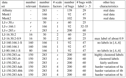
data number number # scale number # bags with other key
set relevant features factors of bags label> .5 characteristics
Affinity - 283 - 139 29 real data
Musk1 - 166 - 92 47 real data
Musk2 - 166 - 102 39 real data
LJ-r.30.s r 30 s 60 25
LJ-r.166.1 r 166 1 92 32-35
LJ-r.283.s r 283 s 200 60
LJ-16.30.2 16 30 2 60 25
LJ-16.30.2-0.9 16 30 2 60 25 max label of about 0.9
LJ-160.166.1-S 160 166 1 92 47 no labels in [.4,.6]
LJ-160.166.1 160 166 1 92 47
LJ-80.166.1-S 80 166 1 92 47 no labels in [.4,.6]
LJ-150.283.sa 150 283 s 200 60 highly clustered labels
LJ-150.283.sb 150 283 s 200 60 clustered labels
LJ-150.283.sc 150 283 s 200 60 fairly uniform
LJ-150.283.4ah 150 283 4 200 60 harder variation of 4a
LJ-150.283.4bh 150 283 4 200 60 harder variation of 4b
LJ-150.283.4ch 150 283 4 200 60 harder variation of 4c
Table 1: Summary of the data set characteristics.
4. Nearest Neighbor Based Approach
One set of approaches we evaluated is based on the nearest neighbor algorithm. In particular, we consider a multiple-instance variant of unweighted k-NN in which the distance between bags Biand
Bjis defined as the minimum Euclidean distance between a point in Biand a point in Bj. Wang and
Zucker (2000) called this distance measure the minimal Hausdorff distance. In the k-NN algorithm, the prediction made for bag B is the average label of the k closest bags.5 The other approach we used is a variation of citation-kNN (Wang and Zucker, 2000). Given a bag B, the C-nearest citers of B include bag Biif and only if B is one of the C-nearest neighbors (under the minimal Hausdorff
distance) of Bi. Note that the number of C-nearest citers is generally not C. Citation-kNN makes
a prediction for bag Bi by taking the average value of the R-nearest neighbors (using the minimal
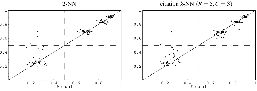
Hausdorff distance)and C-nearest citers. Wang and Zucker found that for the musk data sets the best performance is obtained when R=3 and C=5 and in general recommended having C=R+2. Unless otherwise specified, for citation-kNN we use these values. However, we also did experiments with R=8 and C=10, and since the nearest neighbor information seemed valuable and we wanted to make a fair comparison between 8-NN and citation-kNN. We also performed experiments with R=5 and C=3.
Since the computation of the distance between two points is calculated using all features, when there are many irrelevant features, the distance between two points can be dominated by the irrel-evant features. One way to address this problem is to stretch the axes (shortening the axes corre-sponding to less relevant features and lengthening the axes correcorre-sponding to more relevant features). We refer to s1,...,snas the scale (or relevance) factors where sidefines the relevance of feature i in
computing the target value. Using the artificial data, we compared the results obtained when using (1) the true scale factors (i.e. those that yield theεk values used in generating the data) to rescale
the axes (“true”), (2) when projecting out all features with a scale factor less than 1/2 (“highly rel-evant”), and (3) when projecting out all features with a scale factor of 0 (“relevant”). For both (2) and (3), there is no rescaling of the axes for the features that are used.
We have used a very simple heuristic based on the MULTINST algorithm (Auer, 1997) to es-timate which features are relevant, and then project out those features which we eses-timated to be irrelevant. To estimate whether dimension d is relevant, we project the points onto dimension d and apply a low-pass filter by averaging the values of points nearby in this dimension to eliminate jitter. If the resulting graph has exactly one peak, we estimate that this is a relevant dimension and other-wise we set the scale factor to 0. The results are very preliminary, but in some cases we obtained an improvement to using no scaling.
Observe that both citation-kNN and the k-NN algorithm, when used with minimal Hausdorff metric, are designed for the multiple-instance setting. Not surprisingly, our results demonstrate that both of these k-NN variations significantly outperform the NN-baseline which simply uses the Euclidean distance and ignores the division of the points into bags by just giving each point the label of the bag from which it came.
We now briefly explore the advantages and disadvantages of citation-kNN versus using the k-NN algorithm with the minimal Hausdorff metric. To do this, we first consider the following “idealistic” setting in which there is a very small dense region around the target point for which strong binding (i.e. a label near 1) will occur. Second, assume that there is some distribution
D
over the n-dimensional space with no weight near the target point from which each point from the negative bags are drawn and all but one point from the positive bags are drawn. That is, we assume that with the exception of the one conformation of each drug with strong binding that defines the label, the distribution over the other conformations of drugs that have strong binding are not any different from the conformations taken by drugs that do not bind.6 Since the points are in very high-dimensional space, we assume that any two points drawn fromD
are much further from each other than the diameter of the dense region around the target for which strong binding occurs. Finally, to simplify the analysis, we consider the situation in which the bag size, r, approaches infinity.We also want to bring into our analysis the changes caused by the scale factors being wrong. We make the assumption that if the scale were correct then, with probability 1, a positive bag will have has as its k nearest neighbors other positive bags. To capture the fact that when the scale factors are not correct the dense region of positive points is stretched incorrectly and thus some positive bags are likely to have negative bags as their nearest neighbors, we introduce a parameter 0≤ε≤1 where a positive bag is expected to have k(1−ε)of its k-nearest neighbors be positive bags with the remaining kεneighbors being negative bags. Whenε=0, we model the situation when the scale factors are correct and asεincreases this models increasingly more errors in the estimation of the scale factors.
Next, consider a negative bag. Observe that as the bag size approaches infinity, the nearest neighbor of a negative bag is equally likely to be any of the points that are not in the dense region around the target. Let m+(respectively, m−) be the number of positive bags (respectively, negative bags), let p+=m+/(m++m−) (respectively p−=m−/(m++m−) =1−p+) be the fraction of examples that are positive (respectively, negative), and let r be the size of a bag. Then among the k nearest neighbors of a negative bag, one expects krm−/((r−1)m++rm−) of them to be negative. This follows since there are rm−points from negative bags which are equally likely to be selected among the rm− points from the negative bags and the(r−1)m+ points from the positive bags which are not the point in the bag near the target.7 Thus as r approaches infinity, one expects km−/(m++m−) =k p−=k(1−p+) of the k-nearest neighbors of a negative bag to be negative bags. The remaining k p+ of the k-nearest neighbors of a negative bag will be positive bags. So depending on the fraction of examples which are positive, there can be a very high false positive error rate.
Under the above assumptions, the k-NN algorithm has an accuracy of (1−ε) on the positive bags and an accuracy of p−on the negative bags. Hence the overall accuracy is p+(1−ε)+p2−. So as p+ goes from 0 to 1, the accuracy begins at 1.0 and drops down to a low typically a little less than(1−ε)and then rises back up to 1−εwhen p+reaches 1.
We now consider how the use of citers as done in citation-kNN changes the performance. We assume that k nearest citers are used. If we instead use the k+2 nearest citers as done by Wang and Zucker (2000) then for small k the citers would have slightly more influence in the overall prediction than that given by our analysis here. This would accentuate the differences seen between the two algorithms. When using citers, the problem of misclassifying negative examples is reduced since the citers of a negative bag are very likely to be a negative bag since positive bags are very likely to cite another positive bag. We now compute the expected number of positive and negative citers for both positive and negative bags. From the mp+positive bags, we expect k(1−ε)mp+positive bags to be cited. Dividing these evenly among the mp+positive bags, we expect k(1−ε)positive citers for each positive bag. Similarly, we expect k p− negative citers for each positive bag. Hence for a positive bag the expected accuracy is 2k(1−ε)/(2k(1−ε)+kε+k p−) =2(1−ε)/(2+p−−ε)since this is the sum of the number of citers and neighbors that are positive divided by the total number of neighbors and citers. Similarly, one can compute that the expected accuracy on the negative bags is 2p−/(2p−+p++ε). Thus the overall accuracy would be 2p+(1−ε)/(2+p−−ε) +2p2−/(2p−+ p++ε).
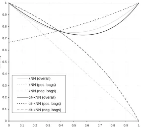
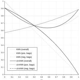
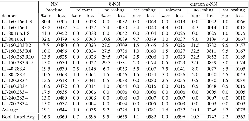
In Figures 1, 2, and 3, we plot these formulas for the accuracy on the positive and negative bags along with the resulting overall accuracy of both k-NN and citation-kNN for values ofεof 0.0, 0.2 and 0.4. From these plots, the following observations can be made. First, whenε=0, for small values for p+ (until approximately 0.4) citation-kNN would be expected to slightly outperform k-NN. For larger values or p+, k-NN has the better performance. Intuitively this occurs because when p+is small then a large fraction of the examples are negative and hence the reduction in the accuracy for positive bags is outweighed by the increase in accuracy for the negative bags. Asεincreases, this relationship changes with k-NN performing better when p+ is small and citation-kNN performing better for larger p+. When p+ is small, k-NN’s performance is fairly insensitive toε since when the scale factors are wrong causing the dense positive region to not appear very dense, the accuracy when predicting the value of negative bags is not affected. However, citation-kNN’s performance
0 0.1 0.2 0.3 0.4 0.5 0.6 0.7 0.8 0.9 1
0 0.1 0.2 0.3 0.4 0.5 0.6 0.7 0.8 0.9 1
p+
accuracy
kNN (overall) kNN (pos. bags) kNN (neg. bags) cit-kNN (overall) cit-kNN (pos. bags) cit-kNN (neg. bags)
Figure 1: Accuracy of k-NN and citation-kNN forε=0.0 for the analytical analysis we performed.
degrades asεincreases since the citers provide much less valuable information. On the other hand, when p+ is larger, citation-kNN performance only decreases a little asεgrows due to the nearest neighbors of the positive bags being more likely to be negative since the citers are still accurate. The accuracy of k-NN drops significantly because it is dominated by the 1−εaccuracy on the positive bags.
The above analysis makes many simplifying assumptions. However, even under these idealistic settings one can clearly see that in some situations k-NN, when using the minimal Hausdorff met-ric (which is quite different from using standard k-NN on the individual points), will outperform citation-kNN while in others citation-kNN will perform best. Although citers were found to im-prove performance for the musk data sets, in general they may not imim-prove performance. Also this analysis considers the accuracy for data with Boolean labels and for which Boolean predictions are made. While, a much more complex analysis would be needed to truly understand the trade-offs between these two approaches in terms of the squared loss, this simple analysis provides some an-alytical grounding to think about the tradeoff between these two approaches which are based upon the nearest neighbor algorithm.
5. Diverse Density Based Approach
0 0.1 0.2 0.3 0.4 0.5 0.6 0.7 0.8 0.9 1
0 0.1 0.2 0.3 0.4 0.5 0.6 0.7 0.8 0.9 1
p+
accuracy
kNN (overall)
kNN (pos. bags)
kNN (neg. bags)
cit-kNN (overall)
cit-kNN (pos. bags)
cit-kNN (neg. bags)
Figure 2: Accuracy of k-NN and citation-kNN forε=0.2 for the analytical analysis we performed.
in feature space. A high diverse density indicates a good candidate for a “true” concept. Let B={hB1,`1i,...,hBi,`ii,...,hBb,`bi}be the training data. Let Bi j denote the jthinstance of bag i,
and Bi jkdenote the feature value of instance Bi j on feature k. The diverse density of possible target
point t is defined as
DD(t) =Pr(t|B) =Pr(B|t)Pr(t)/Pr(B).
We assume uniform priors and so the goal is to search for a t that maximizes Pr(B|t). Assuming the points in B are independent yields
Pr(B|t) =
r
∏
i=1
Pr(Bi|t).
By Bayes’ rule,
Pr(Bi|t) =Pr(t|Bi)Pr(Bi)/Pr(t).
We assume a uniform prior on the targets and that Pr(Bi)is constant with respect to t. Hence the
goal is to maximize ∏bi=1Pr(t|Bi). The key modification required in moving to the real-valued
setting is in estimating Pr(t|Bi). We let
Pr(t|Bi) = (1− |`i−Label(Bi|t)|)/Z
0 0.1 0.2 0.3 0.4 0.5 0.6 0.7 0.8 0.9 1
0 0.1 0.2 0.3 0.4 0.5 0.6 0.7 0.8 0.9 1
p+
accuracy
kNN (overall)
kNN (pos. bags)
kNN (neg. bags)
cit-kNN (overall)
cit-kNN (pos. bags)
cit-kNN (neg. bags)
Figure 3: Accuracy of k-NN and citation-kNN forε=0.4 for the analytical analysis we performed.
We consider two formulas for Label(Bi|t). The first is that of Maron (1999) in which
Label(Bi|t) =max j
( exp(−
n
∑
d=1
(sd(Bi jd−td))2)
)
(2)
where the target is defined by feature values t1,...,tnand scale factors s1,...,sn, and the softmax
is used to approximate the maximum so that it can be differentiated. If each`i∈ {0,1}and we use
Equation (2), then our algorithm reduces to the standard diverse density algorithm. We also tried used the LJ formula by setting Label(Bi|t) =EBi/Emax.
The point t that maximizes∏bi=1Pr(t|Bi)is found using a gradient ascent search over the 2n
di-mensional space defined by t1,...,tn,s1,...,snusing as multiple starting points the features t1,...,tn
from each point in a bag with the maximum label and 0.1 for each si.
6. Empirical Results
For the nearest neighbor algorithms we use leave-one-out cross validation and for diverse density we used 10-fold cross validation.8
NN 8-NN citation k-NN
baseline relevant no scaling est. scaling relevant no scaling est. scaling
data set %err loss %err loss %err loss %err loss %err loss %err loss %err loss
LJ-160.166.1-S 30.4 .0705 0.0 .0028 0.0 .0032 0.0 .0063 0.0 .0013 0.0 .0022 1.0 .0066
LJ-160.166.1 35.8 .0477 5.4 .0027 5.4 .0030 5.4 .0040 4.3 .0011 4.3 .0014 1.0 .0018
LJ-80.166.1-S 41.3 .0952 0.0 .0038 0.0 .0042 0.0 .0104 0.0 .0025 0.0 .0025 1.0 .0075
LJ-80.166.1 32.6 .0479 6.5 .0063 10.8 .0089 9.7 .0079 1.0 .0037 8.6 .0109 4.3 .0067
LJ-150.283.R2 7.5 .0480 0.0 .0023 27.5 .0709 1.5 .0165 3.5 .0026 31.5 .0782 9.5 .0157
LJ-150.283.R4 10.0 .0496 0.0 .0024 27.5 .0736 1.0 .0160 1.5 .0027 32.5 .0811 9.5 .0167
LJ-150.283.R10 13.5 .0525 0.0 .0026 29.5 .0774 2.5 .0206 1.0 .0029 32.5 .0852 7.0 .0185
LJ-150.283.R15 15.0 .0530 0.0 .0027 29.5 .0781 2.0 .0174 0.5 .0029 32.0 .0859 8.0 .0174
LJ-40.283.4 19.5 .0530 2.5 .0146 6.0 .0053 5.5 .0107 7.5 .0141 8.0 .0077 8.5 .0105
LJ-80.283.4 10.5 .0463 1.0 .0064 1.5 .0046 1.5 .0054 3.0 .0056 2.0 .0050 4.5 .0043
LJ-120.283.4 15.5 .0518 0.5 .0041 0.5 .0038 0.0 .0030 2.5 .0055 0.5 .0030 1.5 .0039
LJ-160.283.4 10.5 .0472 0.0 .0014 1.0 .0044 0.0 .0016 0.0 .0016 0.5 .0048 0.5 .0015
LJ-200.283.4 17.5 .0535 0.0 .0006 0.0 .0006 0.0 .0006 0.0 .0006 0.0 .0005 0.0 .0005
LJ-240.283.4 13.0 .0480 0.0 .0006 0.0 .0006 0.0 .0007 0.0 .0007 0.0 .0007 0.0 .0010
LJ-280.283.4 15.0 .0532 0.0 .0004 0.0 .0004 0.0 .0005 0.0 .0003 0.0 .0003 0.0 .0003
Average 19.1 .0544 1.0 .0035 9.2 .0226 1.9 .0081 1.6 .0032 10.1 .0246 3.7 .0075
Bool. Label Avg. 16.9 .0960 0.7 .0596 9.5 .0655 1.1 .0582 0.9 .0596 10.3 .0742 2.2 .0563
Table 2: Overview of nearest neighbor and citation k-NN (for R=3 and C=5) results when using real-valued data. When using the random base the average prediction error was 46.1% and the average squared loss was.1433. The last line of the table shows the average prediction error and squared loss for when the labels are rounded to 0 or 1 (i.e. Boolean labels). For the Boolean setting, the random base had an average prediction error of 46.1% and an average squared loss of.3065.
6.1 Nearest Neighbor Results
We begin with an overview of results using both the nearest neighbor and citation k-NN algorithms when we vary the number of relevant features and whether or not we use a “strong” data set in which there are no examples with labels between 0.36 and 0.77. These results can be found in Table 2. The three columns under both 8-NN and citation k-NN show results for different methods of selecting the scaling factors used for the importance of each feature in the distance computation. The nearest neighbor and citation k-NN algorithms both significantly outperformed both baselines. Between the two baselines, the NN baseline performed significantly better than the baseline obtained by predicting based on the label of a random bag. This relationship occurs in all the data sets and so we only show the NN baseline for the remaining tables. On these data sets, we tested 2-NN, 8-NN,
and citation-kNN (with R=3 and C=5). 8-NN performed approximately 75% better than 2-NN in terms of both the prediction error and squared loss and hence we do not report those results. The performance of 8-NN and citation-kNN are very similar which is very different than what is found when using the musk data sets. For Musk1, 8-NN has error 20.7% whereas citation-kNN has error 10.9%. Similarly, for Musk2, 8-NN has error 27.5% whereas citation-kNN has error 14.7%. Further studies are needed to explain why the results for the musk data sets are different in this respect than for our artificial data sets.
Looking further at the second half of Table 2 it can be seen that the performance dramatically improves as the number of relevant features increases. We believe that the strong performance with respect to the prediction error rate on the musk data sets is partly due to the fact that most of the features are likely to be relevant and that it is a “strong” data set. Finally, in the last two rows we show the average performance when using real values and compare those results to the average performance when using Boolean values (obtained by treating all labels<0.5 as negative and the rest as positive). Not surprisingly, the loss is significantly reduced when using real-valued labels. What is a bit surprising is that the prediction error is sometimes reduced by using the Boolean labels versus the real-valued labels. The reason for this phenomena is that by using labels of 0 or 1 then the predictions tend to be away from 1/2 which increases the loss a lot but helps to keep the prediction on the correct side of the 0.5 threshold.
Next we focus on the effect of varying the number of degrees of relevance. These results can be found in Tables 3– 7. The leftmost column gives the squared loss for the NN baseline. The next two columns show the results when the axes are not re-scaled (i.e. all features are treated as equally relevant). The third column gives the performance when our estimation technique is used to estimate which features are relevant. Then the features estimated to be irrelevant are not used in the distance computation and the rest are treated equally. We then show three columns in which we use knowledge of the trueεvalues to compute the correct scale factors for re-scaling the axes. In the column labeled “use only relevant” we perform the procedure which that estimation technique is trying to do. All of the irrelevant features are not used in the distance computation (and the rest are treated equally). In the column labeled “only use highly relevant” all of the features in which the correct scale factors are at least 1/2 are used. Finally, the column labeled “true scaling” re-scales the axes based on the true scale factors. Thus as we move to the right, we are using more and more detailed information about the true levels of relevance of the features. We include these last three columns to help provide insight into what gains could be made if accurate scale factors could be estimated.
NN no estimated use only use only true baseline scaling scaling relevant highly rel. scaling
LJ-150.283.2a .0956 .0044 .0030 .0032 .0032 .0018
LJ-150.283.4a .0928 .0043 .0033 .0032 .0052 .0022
LJ-150.283.10a .0960 .0056 .0042 .0047 .0032 .0023
LJ-150.283.15a .0967 .0057 .0043 .0048 .0026 .0025
LJ-150.283.4ah .0986 .0071 .0060 .0063 .0075 .0022
LJ-150.283.2b .0945 .0046 .0063 .0064 .0064 .0016
LJ-150.283.4b .0922 .0048 .0067 .0065 .0066 .0038
LJ-150.283.10b .0956 .0070 .0074 .0084 .0058 .0057
LJ-150.283.15b .0963 .0074 .0077 .0088 .0055 .0058
LJ-150.283.4bh .0980 .0098 .0065 .0103 .0095 .0050
LJ-150.283.2c .0374 .0100 .0091 .0080 .0080 .0056
LJ-150.283.4c .0352 .0100 .0072 .0072 .0085 .0067
LJ-150.283.10c .0486 .0136 .0100 .0089 .0086 .0067
LJ-150.283.15c .0506 .0138 .0097 .0089 .0082 .0062
LJ-150.283.4ch .0611 .0161 .0091 .0109 .0102 .0040
Table 3: Performance of 2-NN when varying the number of levels of relevance as measured by the squared loss.
The performance of 2-NN and 8-NN are fairly similar with 8-NN performing slightly better than 2-NN on the easier data sets but with more significant differences on the more complex data sets. Citation k-NN with 3 citers and 5 neighbors outperforms 8-NN. Using 5-citers and 3 neighbors yielded improvements on the easiest “a” data sets but there was a slight degradation in performance on the other data sets. As the data becomes more clustered then the nearest neighbor provides more information and hence the need for citers is reduced. Finally, using 10 citers and 8 neighbors gave the best overall performance.
Next we take a more in-depth look at 2-NN versus citation k-NN with 3 citers and 5 neighbors on the “4ah” data sets. In the plots of Figures 4– 9 we present plots of the predicted label (y-axis) versus the actual label (x-axis). These plots provide more detail than just reporting the squared loss. In each plot we show the 2-NN result on the left and the citation k-NN result on the right. The “4bh” data sets are very similar to the “4ah” data sets and so we don’t show them here. In Figure 10 we look at two plots for the “4ch” data sets to show the different characteristics that these data sets have.
Figure 11 shows the results obtained using Citation-kNN on the Affinity data with Boolean labels (on the left) and with real-valued labels (on the right). In the Affinity set all of the negative labels are clustered near 0.4 and we believe this is part of the reason why the performance is better. Further tests are needed to verify this theory.
NN no estimated use only use only true baseline scaling scaling relevant highly rel. scaling
LJ-150.283.2a .0565 .0036 .0034 .0031 .0031 .0016
LJ-150.283.4a .0554 .0037 .0037 .0033 .0041 .0019
LJ-150.283.10a .0612 .0054 .0053 .0049 .0036 .0019
LJ-150.283.15a .0621 .0056 .0056 .0051 .0026 .0018
LJ-150.283.4ah .0662 .0070 .0077 .0066 .0052 .0019
LJ-150.283.2b .0563 .0049 .0056 .0053 .0053 .0021
LJ-150.283.4b .0555 .0048 .0057 .0056 .0059 .0023
LJ-150.283.10b .0612 .0066 .0074 .0078 .0053 .0024
LJ-150.283.15b .0622 .0067 .0077 .0081 .0042 .0023
LJ-150.283.4bh .0658 .0084 .0095 .0102 .0076 .0019
LJ-150.283.2c .0184 .0090 .0066 .0059 .0059 .0049
LJ-150.283.4c .0187 .0088 .0059 .0063 .0055 .0054
LJ-150.283.10c .0289 .0123 .0078 .0081 .0079 .0044
LJ-150.283.15c .0301 .0124 .0089 .0082 .0080 .0046
LJ-150.283.4ch .0356 .0151 .0092 .0100 .0104 .0050
Table 4: Performance of 8-NN when varying the number of levels of relevance as measured by the squared loss.
2-NN citation k-NN(R=5,C=3)
0.2 0.4 0.6 0.8 1
Actual 0.2
0.4 0.6 0.8 1
P
0.2 0.4 0.6 0.8 1
Actual 0.2
0.4 0.6 0.8 1
P
Figure 4: Predictions on “4ah” data sets for NN baseline. In each of these plots the x-axis corre-sponds to the actual label and the y-axis gives the predicted label.
NN no estimated use only use only true baseline scaling scaling relevant highly rel. scaling
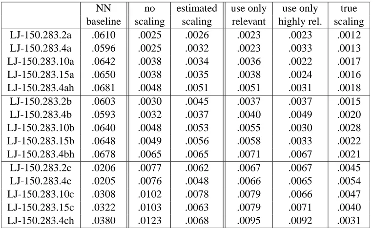
LJ-150.283.2a .0610 .0025 .0026 .0023 .0023 .0012
LJ-150.283.4a .0596 .0025 .0032 .0023 .0033 .0013
LJ-150.283.10a .0642 .0038 .0034 .0036 .0022 .0017
LJ-150.283.15a .0650 .0038 .0035 .0038 .0024 .0016
LJ-150.283.4ah .0681 .0048 .0051 .0051 .0031 .0018
LJ-150.283.2b .0603 .0030 .0045 .0037 .0037 .0015
LJ-150.283.4b .0593 .0032 .0037 .0040 .0049 .0020
LJ-150.283.10b .0640 .0048 .0053 .0055 .0030 .0028
LJ-150.283.15b .0648 .0049 .0056 .0058 .0033 .0022
LJ-150.283.4bh .0678 .0065 .0065 .0071 .0067 .0021
LJ-150.283.2c .0206 .0077 .0062 .0067 .0067 .0045
LJ-150.283.4c .0205 .0076 .0048 .0066 .0065 .0054
LJ-150.283.10c .0308 .0102 .0078 .0079 .0066 .0047
LJ-150.283.15c .0322 .0103 .0063 .0079 .0071 .0040
LJ-150.283.4ch .0380 .0123 .0068 .0095 .0092 .0031
Table 5: Performance of citation k-NN with 3 citers and 5 neighbors when varying the number of levels of relevance as measured by the squared loss.
2-NN citation k-NN(R=5,C=3)
0.2 0.4 0.6 0.8 1
Actual 0.2
0.4 0.6 0.8 1
P
0.2 0.4 0.6 0.8 1
Actual 0.2
0.4 0.6 0.8 1
P
Figure 5: Predictions on “4ah” data sets when no scaling is used (i.e. unweighted distance metric)
6.2 Diverse Density Results
NN no estimated use only use only true baseline scaling scaling relevant highly rel. scaling
LJ-150.283.2a .0651 .0024 .0022 .0022 .0022 .0013
LJ-150.283.4a .0638 .0025 .0031 .0021 .0035 .0014
LJ-150.283.10a .0689 .0033 .0030 .0033 .0024 .0021
LJ-150.283.15a .0699 .0033 .0031 .0033 .0027 .0017
LJ-150.283.4ah .0740 .0040 .0043 .0044 .0030 .0017
LJ-150.283.2b .0645 .0032 .0046 .0040 .0040 .0019
LJ-150.283.4b .0634 .0033 .0044 .0041 .0050 .0025
LJ-150.283.10b .0687 .0049 .0054 .0056 .0032 .0026
LJ-150.283.15b .0696 .0051 .0057 .0058 .0036 .0027
LJ-150.283.4bh .0737 .0067 .0056 .0071 .0060 .0026
LJ-150.283.2c .0241 .0080 .0067 .0065 .0065 .0055
LJ-150.283.4c .0236 .0080 .0049 .0063 .0073 .0055
LJ-150.283.10c .0343 .0105 .0081 .0073 .0066 .0054
LJ-150.283.15c .0357 .0105 .0071 .0073 .0079 .0053
LJ-150.283.4ch .0422 .0125 .0067 .0089 .0092 .0037
Table 6: Performance of citation k-NN with 5 citers and 3 neighbors when varying the number of levels of relevance as measured by the squared loss.
2-NN citation k-NN(R=5,C=3)
0.2 0.4 0.6 0.8 1
Actual 0.2
0.4 0.6 0.8 1
P
0.2 0.4 0.6 0.8 1
Actual 0.2
0.4 0.6 0.8 1
P
Figure 6: Predictions on “4ah” data sets when our estimation method is used to estimate which fea-tures are relevant. Only the feafea-tures estimated to be relevant are used (weighted equally).
NN no estimated use only use only true baseline scaling scaling relevant highly rel. scaling
LJ-150.283.2a .0529 .0026 .0026 .0022 .0022 .0011
LJ-150.283.4a .0521 .0026 .0027 .0023 .0027 .0013
LJ-150.283.10a .0581 .0039 .0037 .0034 .0021 .0015
LJ-150.283.15a .0591 .0040 .0039 .0035 .0017 .0013
LJ-150.283.4ah .0634 .0051 .0051 .0046 .0030 .0013
LJ-150.283.2b .0524 .0030 .0034 .0027 .0027 .0014
LJ-150.283.4b .0520 .0030 .0036 .0029 .0036 .0016
LJ-150.283.10b .0580 .0045 .0048 .0040 .0034 .0016
LJ-150.283.15b .0590 .0046 .0050 .0041 .0028 .0016
LJ-150.283.4bh .0632 .0061 .0058 .0053 .0058 .0016
LJ-150.283.2c .0185 .0086 .0057 .0055 .0055 .0042
LJ-150.283.4c .0187 .0084 .0051 .0057 .0048 .0046
LJ-150.283.10c .0285 .0112 .0062 .0070 .0065 .0033
LJ-150.283.15c .0297 .0113 .0069 .0071 .0062 .0037
LJ-150.283.4ch .0348 .0135 .0065 .0084 .0082 .0036
Table 7: Performance of citation k-NN with 10 citers and 8 neighbors when varying the number of levels of relevance as measured by the squared loss.
2-NN citation k-NN(R=5,C=3)
0.2 0.4 0.6 0.8 1
Actual 0.2
0.4 0.6 0.8 1
P
0.2 0.4 0.6 0.8 1
Actual 0.2
0.4 0.6 0.8 1
P
Figure 7: Predictions on “4ah” data sets when knowledge of the true scale factors are used to only use the truly relevant features (weighted equally).
2-NN citation k-NN(R=5,C=3)
0.2 0.4 0.6 0.8 1
Actual 0.2
0.4 0.6 0.8 1
P
0.2 0.4 0.6 0.8 1
Actual 0.2
0.4 0.6 0.8 1
P
Figure 8: Predictions on “4ah” data sets when knowledge of true scale factors are used to only use the relevant features with scale factors at least 0.5 (weighted equally).
2-NN citation k-NN(R=5,C=3)
0.2 0.4 0.6 0.8 1
Actual 0.2
0.4 0.6 0.8 1
P
0.2 0.4 0.6 0.8 1
Actual 0.2
0.4 0.6 0.8 1
P
Figure 9: Predictions on “4ah” data sets when the true scale factors are used to re-scale the axes.
then the search stops after only a few rounds and the scale factors are not able to adjust. However, when the maximum label is 0.9 there is “more room” for the search procedure to work and hence the results are better.
0.2 0.4 0.6 0.8 1 Actual
0.2 0.4 0.6 0.8 1
P
0.2 0.4 0.6 0.8 1
Actual 0.2
0.4 0.6 0.8 1
P
Figure 10: Predictions on “4ch” data sets made by citation k-NN with 5 neighbors and 3 citers. The plot on the left uses the actual scale factors and the plot on the right uses our estimation procedure.
Boolean labels real-valued labels
0.2 0.4 0.6 0.8 1
Actual 0.2
0.4 0.6 0.8 1
Predicted
0.2 0.4 0.6 0.8 1
Actual 0.2
0.4 0.6 0.8 1
P
Figure 11: Results from using citation-kNN on the Affinity data set.
Diverse Density citation-kNN
data set %err loss %err loss
LJ-160.166.1-S 0.0 .0052 0.0 .0022 LJ-160.166.1 23.9 .0852 4.3 .0014 LJ-80.166.1-S 53.3 .1116 0.0 .0025 LJ-16.30.2-0.9 6.7 .0071 8.3 .0197
LJ-16.30.2 6.7 .0240 16.7 .0260
Affinity 26.8 .0421 14.4 .0124
Table 8: Comparison of results of diverse density (where all scale factors are initially 0.1) and citation-kNN with no scaling when using real-valued labels.
Diverse Density citation-kNN
data set %err loss %err loss
LJ-160.166.1-S 4.3 .0278 0.0 .0463 LJ-160.166.1 12.0 .0904 2.2 .0750 LJ-80.166.1-S 51.1 .1140 0.0 .0444 LJ-16.30.2-0.9 11.7 .0736 5.0 .0359
LJ-16.30.2 13.3 .0731 18.3 .0403
Table 9: Comparison of results of diverse density (where all scale factors are initially 0.1) and citation-kNN with no scaling when using Boolean labels.
7. Concluding Remarks
In this paper we present extensions of nearest neighbor and diverse density algorithms for the real-valued setting. Our initial studies have provided some important insights into these algorithms. The performance of both the nearest neighbor and diverse density algorithms are very sensitive to the number of relevant features. When most of the features are relevant the performance is quite good and degrades as a larger fraction of the features become irrelevant. There is also some dependence on the number of different scale factors but this has a smaller effect on performance than the number of relevant features. (Both of these phenomena can be seen for the nearest neighbor algorithms in the results shown in Table 2.) We believe that good performance has been obtained on the musk data sets partly because a significant fraction of the features are relevant. For 2-NN, 8-NN, and several variations of citation-kNN we showed how performance is affected as we vary the number of relevant features, the degree of relevance, the distributional features of the data, and the learning algorithm.
LJ-16.30.2-T LJ-16.30.2-0.9 LJ-16.30.2
0.2 0.4 0.6 0.8 1
Actual 0.2 0.4 0.6 0.8 1 Predicted
0.2 0.4 0.6 0.8 1
Actual 0.2 0.4 0.6 0.8 1 Predicted
0.2 0.4 0.6 0.8 1
Actual 0.2 0.4 0.6 0.8 1 Predicted
Figure 12: Results obtained when using the diverse density algorithm for real-valued data. In data set LJ-16.30.2-T, all features values including the irrelevant features are selected based on the target point versus the standard method in which the irrelevant features are ran-domly selected.
LJ-160.166.1-S LJ-160.166.1 LJ-80.166.1-S
0.2 0.4 0.6 0.8 1
Actual 0.2 0.4 0.6 0.8 1 Predicted
0.2 0.4 0.6 0.8 1
Actual 0.2 0.4 0.6 0.8 1 Predicted
0.2 0.4 0.6 0.8 1
Actual 0.2 0.4 0.6 0.8 1 Predicted
Figure 13: Results obtained when using the diverse density algorithm for real-valued data.
that these values have basically no correlation to the real values. We believe the reason for this phenomena is that scale factors are found that increase performance for a local optimum in the gradient ascent search. We have provided a heuristic to estimate which features are relevant, but much more research in this direction is needed. Perhaps the diverse density search heuristic could be adapted to accelerate the search and obtain final scale factors that correlate better with the true scale factors. Having artificial data sets in which the true scale factors are known will be very valuable in evaluating the effectiveness of different algorithms to estimate which features are relevant.
Acknowledgments
We would like to acknowledge support for this project from the National Science Foundation (NSF grant CCR-9988314 and an REU supplement). We also thank the anonymous reviewers for their helpful comments, and Craig Codrington for a careful reading of this manuscript in which many typographical corrections and improvements were suggested. Daniel Dooly and Robert Amar per-formed this work while at Washington University. An earlier version of this paper appeared in ICML 2001.
Appendix
Here is the pseudo-code used to generate the artificial data. In this pseudo-codo i is the index for the molecule. Also, this pseudo-code is for the LJ-150.283 data sets. Others were generated in a similar fashion except that the number of attributes (283) and relevant attributes (150) were varied.
The below procedure generates values for index[0],index[1], and index[2]. The method to assign the attribute values to the features that fall in the ranges which end at index[0], index[1], and index[2] is described in the body of the paper. The method described in the paper along with the method used below to define index[0],index[1],index[2]is used to generate the shape of the molecule responsible for the label in the “0.9” data sets in which there is no label with value of 1.0. For the data sets in which there is a label of 1.0, for the case when i=0, a molecule is generated that has the exact target value for each relevant attribute. Finallyrand0andrand1are both a random number generate uniformly from[0,1].
For the "a" data set: if (i<3){
index[0] = 150; index[1] = 150; index[2] = 150; }else if (i<10){
tmp0 = (int)(100+50*rand0);
index[0] = tmp0; index[1] = 150; index[2] = 150; }else if (i<30){
tmp0=(int)(25+5*rand0); tmp1=(int)(125+25*rand1);
index[0] = tmp0; index[1] = tmp1; index[2] = 150; }else if (i<60){
tmp0=(int)(10+5*rand0); tmp1=(int)(60+10*rand1);
index[0] = tmp0; index[1] = tmp1; index[2] = 150; }else if(i<100){
tmp1=(int)(125+25*((rand0+rand1)/2.0));
index[0] = 0; index[1] = 25; index[2] = tmp1; }else if (i<150){
tmp1=(int)(50+100*((rand0+rand1)/2.0)); index[0] = 0; index[1] = 0; index[2] = tmp1; }else{
For the "b" data set: if (i<3){
index[0] = 150; index[1] = 150; index[2] = 150; }else if (i<10){
tmp0=(int)(50+100*rand0);
index[0] = tmp0; index[1] = 150; index[2] = 150; }else if (i<30){
tmp0=(int)(20+10*rand0); tmp1=(int)(100+50*rand1);
index[0] = tmp0; index[1] = tmp1; index[2] = 150; }else if (i<60){
tmp0=(int)(10+5*rand0); tmp1=(int)(60+10*rand1);
index[0] = tmp0; index[1] = tmp1; index[2] = 150; }else if(i<100){
tmp1=(int)(100+50*rand0);
index[0] = 0; index[1] = 25; index[2] = tmp1; }else if (i<150){
tmp1=(int)(50+100*rand1);
index[0] = 0; index[1] = 0; index[2] = tmp1; }else{
index[0] = 0; index[1] = 0; index[2] = 0; }
For the "c" data set: if (i<3) {
index[0] = 50; index[1] = 50; index[2] = 50; }else if (i<10){
tmp0=(int)(20+10*rand0);
index[0] = tmp0; index[1] = 50; index[2] = 50; }else if (i<30){
tmp0=(int)(10+8*rand0); tmp1=(int)(18+10*rand1);
index[0] = tmp0; index[1] = tmp1; index[2] = 50; }else if(i<60){
tmp0=(int)(6+6*rand0); tmp1=(int)(15+10*rand1);
index[0] = 0; index[1] = tmp1; index[2] = 50; }else if (i<100){
tmp0=(int)(10+10*rand0); tmp1=(int)(35+10*rand1);
index[0] = 0; index[1] = tmp0; index[2] = tmp1; }else if (i<150) {
index[0] = 0; index[1] = 0; index[2] = 50; }else{
References
Auer, P. (1997) On learning from mult-instance examples: Empirical evaluation of a theoretical approach. Proceedings 14th International Conference on Machine Learning, (pp. 21–29), San Francisco: Morgan Kaufmann.
Auer, P., Long, P. M. and Srinivasan, A. (1997) Approximating hyper-rectangles: Learning and pseudo-random sets. Proceedings of the Twenty-Ninth Annual ACM Symposium on Theory of Computing (pp. 314–323).
Berry, R.S., Rice, S. A. and Ross, J. (1980). Physical Chemistry, Chapter 10 (Intermolecular Forces). John Wiley & Sons.
Blum, A. and Kalai, A. (1998). A note on learning from multiple-instance examples. Machine Learning, 30, 23–29.
Dietterich, T. G., Lathrop, R. H. and Lozano-P´erez, T. (1997). Solving the multiple-instance prob-lem with axis-parallel rectangles. Artificial Intelligence, 89, 31–71.
Fehr, C., Galindo, J., Haubrichs, R. and and Perret, R. (1989). New aromatic musk odorants: Design and synthesis. Helvetica Chimica Acta, 72, 1537-1553.
Goldman, S.A. and Scott, S.D. (2001). Multiple-Instance Learning of Real-Valued Geometric Pat-terns. To appear in Annals of Mathematics and Artificial Intelligence.
Jain, A.N., Dietterich, T.G., Lathrop, R.H., Chapman, D., Critchlow, R.E., Bauer, B.E., Webster, T.A. and Lozano-P`erez, T. (1994). Compass: A shape-based machine learning tool for drug design. Computer Aided Molecular Design, 8 635–652.
Long, P. M. and Tan, L. (1998) PAC learning axis-aligned rectangles with respect to product distri-butions from multiple-instance examples. Machine Learning, 30, 7–21.
Maron, O. (1998). Learning from Ambiguity. Doctoral dissertation, MIT, AI Technical Report 1639. Maron, O. and Lozano-P´erez, T. (1998). A framework for multiple-instance learning. Neural
Information Processing Systems, 10, MIT Press.
Maron, O. and Ratan, A. (1998). Multiple-instance learning for natural scene classification. Pro-ceedings 15th International Conference on Machine Learning (pp. 341–349). San Francisco: Morgan Kaufmann.
Ray, S. and Page, D. (2001). Multiple instance regression. In Proc. 18th International Conference on Machine Learning, (pp. 425–432). San Francisco: Morgan Kaufmann.
Ruffo, G. (2000). Learning single and multiple instance decision trees for computer security ap-plications. Doctoral dissertation. Department of Computer Science, University of Turin, Torino, Italy.