http://www.sciencepublishinggroup.com/j/ajtas doi: 10.11648/j.ajtas.20190805.14
ISSN: 2326-8999 (Print); ISSN: 2326-9006 (Online)
Analysis of Penalized Regression Methods in a Simple
Linear Model on the High-Dimensional Data
Zari Farhadi
1, Reza Arabi Belaghi
1, Ozlem Gurunlu Alma
2, *1Department of Statistics, University of Tabriz, Tabriz, Iran 2
Department of Statistics, Mughla Sitki Kochman Unv, Mughla, Turkey
Email address:
*
Corresponding author
To cite this article:
Zari Farhadi, Reza Arabi Belaghi, Ozlem Gurunlu Alma. Analysis of Penalized Regression Methods in a Simple Linear Model on the High-Dimensional Data. American Journal of Theoretical and Applied Statistics. Vol. 8, No. 5, 2019, pp. 185-192.
doi: 10.11648/j.ajtas.20190805.14
Received: June 26, 2019; Accepted: August 19, 2019; Published: October 16, 2019
Abstract:
Shrinkage methods for linear regression were developed over the last ten years to reduce the weakness of ordinary least squares (OLS) regression with respect to prediction accuracy. And, high dimensional data are quickly growing in many areas due to the development of technological advances which helps collect data with a large number of variables. In this paper, shrinkage methods were used to evaluate regression coefficients effectively for the high-dimensional multiple regression model, where there were fewer samples than predictors. Also, regularization approaches have become the methods of choice for analyzing such high dimensional data. We used three regulation methods based on penalized regression to select the appropriate model. Lasso, Ridge and Elastic Net have desirable features; they can simultaneously perform the regulation and selection of appropriate predictor variables and estimate their effects. Here, we compared the performance of three regular linear regression methods using cross-validation method to reach the optimal point. Prediction accuracy using the least squares error (MSE) was evaluated. Through conducting a simulation study and studying real data, we found that all three methods are capable to produce appropriate models. The Elastic Net has better prediction accuracy than the rest. However, in the simulation study, the Elastic Net outperformed other two methods and showed a less value in terms of MSE.Keywords:
Shrinkage Estimator, High Dimension, Cross-Validation, Ridge Regression, Elastic Net1. Introduction
With the advancement of technology, data are turning into high-dimensional data that may cause many problems in various research, scientific, medical and engineering fields [10]. Compared to conventional data, this type of data refers to unusual and unstructured data. The analysis of big data requires methods other than the traditional analytical framework [9]. In classical statistical theory, it is assumed that the number of n observations is higher than the number of variables or parameters, but for high-dimensional data the number of variables is greater than the number of observations. The analysis of these data has changed statistical thinking [9].
In many applications, the interested response variable is dependent on a relatively small number of predictors. For
example, in genetic studies using micro arrays, there is myriad predictor gene, but only few of them are the important variables associated with the disease. How to identify "sparse" variables in case of high-dimensional data has become a rudimentary challenge [10].
Hoerl and Kennard introduced ridge regression in 1970 and stated that, despite the correlation between predictor variables, the use of least square cause errors in estimation. He developed ridge regression as an alternative which allows estimations to be done with less variance than the least squares method [11].
(1970) in Ridge's regression research was to introduce this feature. If β has no limitation, it can be very large and extensive. It is therefore they are sensitive to very high variance. To control variance, coefficients can be regulated [5].
Lasso- Least Absolute Shrinkage and Selection Operator- was first proposed by Robert Tibshirani [8] in 1996. Lasso method is a powerful technique that performs two main tasks: regularization and feature selection. In this method, a constraint is put on the sum of the absolute value of model parameters where the sum is less than a fixed value. To do this, a shrinking (regularization) process is applied where the coefficients of the regression variables shrink or some of them reach to zero. During the features selection process, variables that have non-zero coefficients after shrinking process are selected as a part of the model. The purpose of this process is to minimize the prediction error [9].
Zou and Hastie [13] introduced Elastic Net which outperforms Lasso, especially in cases where the number of predictions is significantly larger than the sample size (p >> n), while maintains its sparsity. Elastic net can perform both automatic variable selection and continuous shrinkage simultaneously and select a group of correlated variables. Elastic net can be used as a linear combination of Ridge and Lasso lines. Estimation of elastic net is a two-step method that first defines regression coefficient for each fixed , then conducts a lasso-type shrinkage along the path, which seems to incur a double amount of shrinkage. While double shrinkage does not help to reduce the variances much, it reduces unnecessary values compared to lasso or ridge.
In this paper, we evaluate the performance of three penalized regression methods: Ridge, Lasso, and Elastic Net.
2. The Regularization Models
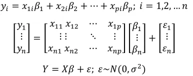
The regression model used to predict the performances of each of the above-mentioned methods are as follows:
= + ; ~ (0, )
where y = (y , y , … , y ) is observation vector, X is n × p Matrix of predictors, β = (β , β , … , β ) is regression coefficients vector and ε is the vector of residual errors with
var(ε) = σ I variance [1].
The least square method provides the estimation of parameters by minimizing the following function:
#$%&'(
), *∑ (,-− )− ∑ /-0 0 1
02 )
3
-2 4 (1)
Usually, the least squares estimate obtained from equation (1) is non-zero, but if p is big, this challenges the interpretation of final model. In fact, if n <p, the estimation of least squares is not unique. Thus, there are different methods that make target function equal to zero. Therefore, it is required to limit or regulate the estimations of coefficients that is called penalty. Penalized regression is used when there are an excessive number of independent variables in the regression or high-dimensional problems (SLS) [8].
2.1. Ridge Regression
Ridge regression [3] is perfect if there are various predictors, all with non-zero coefficients and collect from a normal distribution [6]. In specific, it carry out well with many predictors each having small outcome and prevents coefficients of linear regression models with many correlated predictors from being poorly determined and exhibiting high variance. Ridge regression shrinks the coefficients of correlated predictors equally towards zero.
Equation (2) represents Ridge regression estimator using
ℓ penalized least squares as:
56-789=#$%&'(‖, − ; ‖ + ‖ ‖ (2)
Where ‖, − ; ‖ = ∑ (,3-2 -− ; ) is ℓ -norm loss function, x= is the i-th row of X, ‖ ‖ = ∑102 0 is the ℓ -norm penalty on β and λ ≥ 0 is regulation parameter which regulates penalty (linear shrinkage) by determining the relative importance of the data-dependent error. Since the value λ is depended on the data, cross-validation method can be used [1].
By substituting these values into Equation (2), we have:
#$%&'(
), *∑ (,-− )− ∑ /-0 0 1
02 )
@
-2 4 A. C ∑102 0 ≤ C (3)
Where t is a user-specified parameter.
2.2. Lasso
Lasso is a method that shrinks the loss of absolute error sum of squares and constraints the sum of the absolute value of coefficients. Since the nature of this constraint has a shrinking effect on coefficients and even sets some to zero, it provides proper interpretative regression models automatically [8].
The lasso estimator uses the ℓ penalized least squares basis to obtain a sparse solution to the following optimization problem.
5EFGGH =#$%&'(‖, − ; ‖ + ‖ ‖ (4)
Where ‖ ‖ = ∑102 0 is a norm penalty of ℓ under that expresses the degree of sparsity and ≥ 0 is regulation parameter [1].
Equation (4) can be written as:
#$%&'(
), *∑ (,-− )− ∑ /-0 0 1
02 )
3
-2 4 A. C ∑ I0 0I≤ C (5)
2.3. Elastic Net
Elastic Net is other regularization and variable section method which includes a tuning parameter α ≥ 0 and is the combination of two previous methods (Lasso and Ridge). Elastic Net overcomes the limitations of the Lasso. It deals with the correlation problem of Ridge regression and large selection of variables in the Lasso regression using ℓ and
ℓ penalties. When α = 1, Elastic Net is changed into ridge regression (explained in the previous section). For α ∈ [0,1), the Elastic Net penalty function is singular at zero and it is strictly convex for all α > 0, thus having the characteristics of both the Lasso and Ridge regression. The Lasso penalty is convex but not strictly convex [12].
The Elastic Net uses a combination of ℓ and ℓ penalties and can be defined as:
59EFGP-Q = (1 +RS
@){#$%&'(‖, − ‖ + ‖ ‖ + ‖ ‖ } (6)
On setting α =RRS
VWRS, the estimator of Equation (7) will be similar to the minimizer of:
59EFGP-Q = X1 +RS
@Y {#$%&'(‖, − ‖ + ‖ ‖ + ‖ ‖ } A. C (1 − Z)| | + Z| | ≤ C (7)
Where (1 − Z)‖ ‖ + Z‖ ‖ is the Elastic Net and is the convex combination of Lasso and Ridge penalties [1].
3. Descriptor Data Set
Three states of n and p are investigated. Firstly, the initial data set including n = 35 observations and p = 17 predictions (n > p) are studied. Then, n = 12 observations and p = 17 predictions (n < p) are also studied. Finally, the data set are also calculated when n = p = 17. In this study, the data sets are used from ISLR package on Hitters data available in R software.
3.1. Choosing the Tuning Parameter
The most important point in selecting penalized regression models is choosing a suitable value for the tuning parameters. There are various ways to select the tuning parameter. including:
a. The bootstrap
b.Information criteria like AIC, BIC, RIC c. SURE (Stein's Unbiased Risk Estimate) d.SRM (Structural Risk Minimization) e. Stability-based methods
The most popular one is the cross-validation method and we use it to obtain the tuning parameter. For example, we use a 10-fold cross validation to select the tuning parameter. The intended method includes dividing the data set into 10 identical subsamples i.e. the optimal model is used in 9 subsamples (90 percent of data as training sets) and the evaluation of model performance in the remaining samples (10 percent of data as test set) is studied. Then, this procedure is repeated for each 10 subsamples which are used as validation set once. Finally, a
λ value is selected that has the least mean square error.
In Table 1, the value of λ]=^ and λ _` tuning parameters for each three methods in the three studied states are presented:
Table 1. The value of the tuning parameters for the three methods n = 35, 17, 12 and p = 17.
a > b a = b a < b
cdea cfgh cdea cfgh cdea cfgh
ridge 3104.275 7870.469 264162.4 56568.99 4429.444 8495.276
lasso 46.0975 154.5005 51.85615 165.9017 82.99969 109.7207
elastic 101.1839 256.5381 90.20366 250.9971 22.46051 41.11932
In the Lasso and Ridge regression, the value of λ]=^ in low-dimentional data (( > J) is less than the one in the high-dimentional data (( < J), but λ _`, shows that the standard deviation error has a lower value in the high-dimension. In the elastic net, both values of λ are reduced in
all three states.
Since the constraints applied to the parameters in the Lasso are higher than the elastic net and ridge, the value of λ for the Lasso in all three states ( > J, ( = J and ( < J will be lower than the elastic net and ridge.
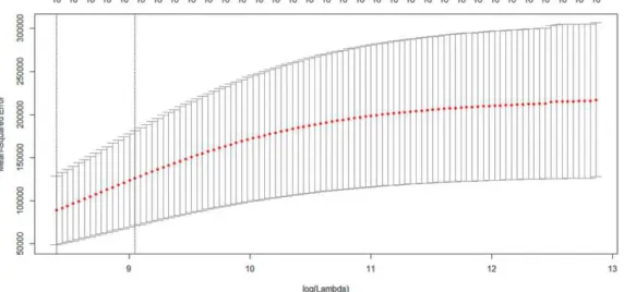
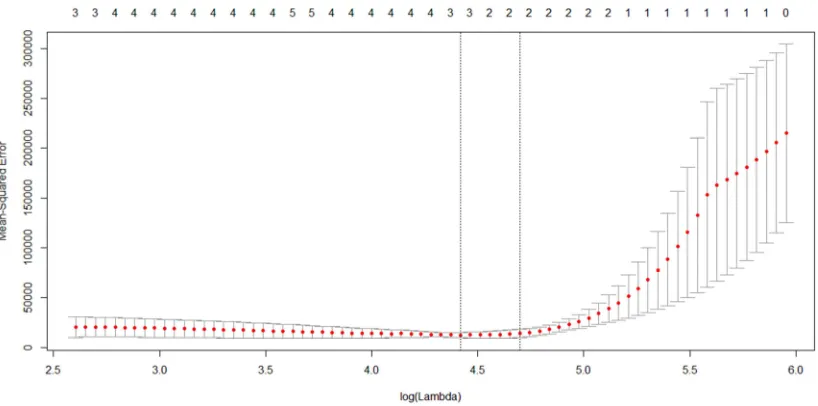
Figure 2. Crass-validation plot of high dimensional data (p=17, n=12)–Lasso.
Figure 3. Crass-validation plot of high dimensional data (p=17, n=12)-Elastic net.
In Figures 1, 2, 3 the red dots are the cross validation error and the top and down lines are the standard deviation. The left vertical dashed line refers to the candidate associated with the minimum MSE, and the right vertical dashed line refers to the largest candidate which is 1 standard deviation away from the minimum MSE. Since λ]=^ had the least
squares mean of the cross validation error, we used this value of to fit the model.
3.2. Fitting and Analyzing Models
Prior to evaluation of each method, at first the data are divided into training and test sets. Training set is defined as a subset of our initial observations used for modeling. In contrast, test set is used as a means for validation and performance evaluation of model resulted from training set. In this way, usually a model in the training set is trained and then model prediction accuracy in the test set model is used to assess model fitting. We divided the data set into 50:50. All results obtained from regression models of Ridge, Lasso
and Elastic Net were calculated by glmnet at R [6]. To investigate optimization fully, 10-fold cross-validation (CV) at Glmnet was used.
4. Results and Discussion
We described several penalized linear regression methods. In this section, we carried out experiments to test the performance of three methods. Penalized methods can bring down the model prediction error to zero by reducing the regression coefficients and lowering the estimates. In all three cases, the data set were divided into training and test sets. The division based on random sample was conducted, in which all models focused only on training set and then they were evaluated on the test set. The values of tuning parameter were also selected according to the explanation presented in sub-section (2.2) through 10-fold cross-validation.
AtBat is 6.095562e-02 and by increasing dimension (( < J) its value were reduced to 0.046772123, which means that values are close to zero.
In all three states, Ridge regression didn’t perform any variable selection and all variables were present in the model
with values close to zero (but not exactly zero).
Table 2 indicates 10 variables selected from 17 covariate variables by Ridge regression and the coefficients estimated from actual data.
Table 2. The estimated coefficients for ridge regression when n = 35, 17, 12 and p = 17.
Covariate a > b a = b a < b
Estimate Estimate Estimate
AtBat 6.095562e-02 0.05210685 0.046772123
Hits 1.957214e-01 0.158989686 0.129869441
HmRun 7.746080e-01 0.604271053 0.677242729
Runs 2.784005e-01 0.263803187 0.201909315
RBI 3.246204e-01 0.287511662 0.322156616
Walks 3.691845e-01 0.491997136 0.459408811
CRuns 3.990050e-02 0.034330322 0.032617473
CAtBat 5.161903e-03 0.004682497 0.005135992
CHits 1.724367e-02 0.015920369 0.017781588
CHmRun 1.458783e-01 0.116790172 0.101384765
Table 3 indicates the variables selected in the lasso model as well as the estimated values for all three states. In J > (,
J = ( and ( > J, Lasso method selects 4, 3 and 3 variables from 17 variables, respectively. Other variables became exactly zero in all three states.
Table 3. The estimated coefficients for lasso regression when n = 35, 17, 12 and p = 17.
a > b a = b a < b
Covariate Estimate Covariate Estimate Covariate Estimate
AtBat 0.3183589 AtBat 0.03368616 Walks 0.34407434
Years 9.197508 Hits 0.14660423 Years 3.49588665
CWalks 0.6141448 CWalks 0.75911681 CAtBat 0.01610091
CWalks 0.54286127
The estimated values for the variables selected in final model are different. The Lasso regression method selected different variables for different states and n & p. The CWalks variable is selected for all three states but its value in the low dimension (( > J) is 0.6141448 and in the high-dimension is 0.54286127. As increasing dimension, the value of the variable decreases and approaches to zero. In cases where the variable
is not suitable for the model, it is exactly equal to zero.
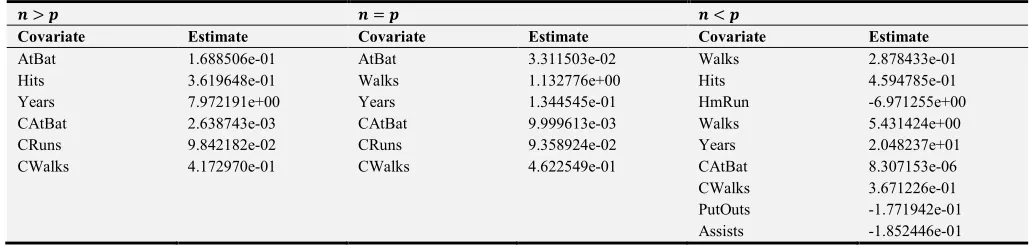
Table 4 indicates the variables selected in Elastic Net as well as the estimated value for all three states. In J > (, J =
( and ( > J, elastic net method selects 9, 6 and 6 variables from 17 variables, respectively. Other variables became exactly zero in all three states.
Table 4. The estimated coefficients for elastic net when n = 35, 17, 12 and p = 17 and α=0.5.
a > b a = b a < b
Covariate Estimate Covariate Estimate Covariate Estimate
AtBat 1.688506e-01 AtBat 3.311503e-02 Walks 2.878433e-01
Hits 3.619648e-01 Walks 1.132776e+00 Hits 4.594785e-01
Years 7.972191e+00 Years 1.344545e-01 HmRun -6.971255e+00
CAtBat 2.638743e-03 CAtBat 9.999613e-03 Walks 5.431424e+00
CRuns 9.842182e-02 CRuns 9.358924e-02 Years 2.048237e+01
CWalks 4.172970e-01 CWalks 4.622549e-01 CAtBat 8.307153e-06
CWalks 3.671226e-01
PutOuts -1.771942e-01
Assists -1.852446e-01
With increasing dimension In the Elastic Net regression, more variables are selected to be in the model because the Elastic Net is group selection, and the obtained values are less or negative, so it had better estimation in the model. Although 9 variables were selected for the model (( < J), but it would be a good fit. The negative values include PutOuts, Assists and HmRun.
According to above tables and obtained results, since
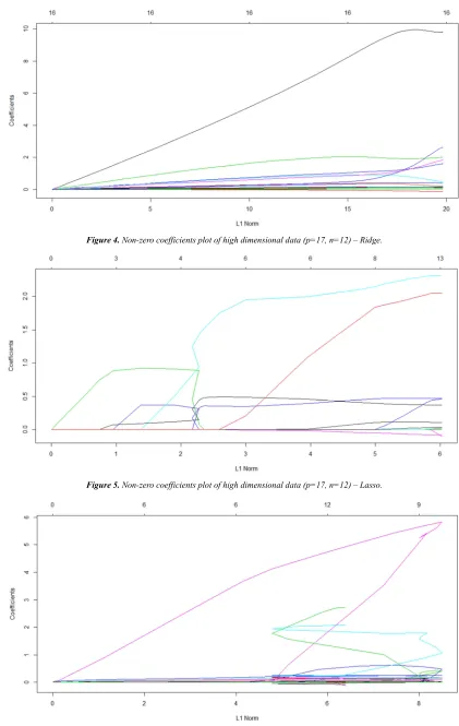
Figure 4. Non-zero coefficients plot of high dimensional data (p=17, n=12) – Ridge.
Figure 5. Non-zero coefficients plot of high dimensional data (p=17, n=12) – Lasso.
Figures 4, 5, 6 shows the regression coefficients of the Ridge, Lasso, Elastic Net. As we can see in the figure, the black color variable in the Ridge regression, the red and cyan color variables in the Lasso regression, and the pink color variable in the Elastic Net regression have the largest effect on the response variable. They are the first variables to enter the model and the subsequent variables with different effects enter the model. Finally, the coefficients of ineffective variables in the model become zero.
5. Simulation Study
Using Monte Carlo simulations, we want to obtain the prediction accuracy of penalized regression methods: Lasso, Ridge and Elastic Net. To do this simulation, the preliminary data from a normal distribution are generated randomly and then the results obtained from these methods are calculated by 500 replications. In this simulation, X =
(x , … , x ) matrix is generated from normal distribution (mean= 2 and variance=0.25) which has been done on the simple linear regression model:
,-= /- + / - + ⋯ + /1- 1; ' = 1,2, … (
l,⋮ ,@
n = l / /⋮ ⋮ ⋯ /⋱ ⋮1 /@ /@ ⋯ /@1
n l ⋮
@
n + l ⋮
@
n
= + ; ~ (0, )
Where regression coefficients are = (2, … 2pqr
G2s , 0, … 01tG2pqr) ;.
The ε values are generated from normal distribution with zero mean and variance of 0.25.
5.1. Case Where p > n
In this state, we confront high-dimensional data, thus the penalized regression methods namely Lasso, Ridge and Elastic net are used. Number of observations and predictors is n = 12 and p = 17, respectively. Based on previous section and the analysis of actual data in Ridge regression, here Ridge regression didn’t perform any variable selection and none of the coefficients became zero. However, Lasso and Elastic Net performed variable selection.
According to Table 5 Lasso and Elastic Net selected 5 variables for the model, but the mean square error in Elastic Net was estimated to be lower than that of Lasso and Ridge.
Table 5. λ and MSE for each of Ridge, Lasso and Elastic net methods with σ = 0.5.
Variables Selection cdea MSE
ridge 546.3457 20.07218 all
lasso 546.155 0.15546 5
elastic 545.9098 0.1308232 5
5.2. Case Where p = n
In this state, the number of observations and predictors is n=17 and p = 17, respectively. Ridge regression did not
perform any type of variable selection and none of coefficients became zero, but Lasso and Elastic Net performed variable selection.
According to Table 6, Lasso and Elastic Net (with σ =
0.5) select 2 and 4 variables, respectively. However, the mean square error is less than that of Lasso and Ridge.
Table 6. λ and MSE for each of Ridge, Lasso and Elastic net methods with σ = 0.5.
Variables Selection cdea MSE
ridge 2831.925 401.4436 all
lasso 2836.371 3.108232 2
elastic 2836.326 6.216464 4
5.3. Case Where p<n
In this state, the number of observations and predictors is n= 35 and p = 17, respectively. Ridge regression did not perform any type of variable selection and none of coefficients became zero, but Lasso and Elastic Net performed variable selection.
According to Table 7, Lasso and Elastic Net (with σ =
0.5) select 11 and 10 variables, respectively. However, the mean square error is less than that of Lasso and Ridge.
Table 7. λ and MSE for each of Ridge, Lasso and Elastic net methods with σ = 0.5.
Variables Selection cdea MSE
ridge 547.309 25.1206 all
lasso 547.671 0.08419426 2
elastic 547.1962 0.2225997 4
From the simulation results, we observed that Lasso had the higher sparsity and less variable selection than the Elastic net in all three states n and p. The parameters were selected with 10-fold cross validation, while having the same level of performance. Although Lasso had less variable selection than Elastic net, but the MSE of Elastic net was less than Lasso in all three states.
The dataset is obtained from the MASS, R package being analysed for the statistical inference purposes such as variable selection, hypothesis tests and the covariance test by some researchers including [7]. The results obtained for the penalized regression performance of the methods, the variable selection was similar to the one that was obtained in our study. In addition to accuracy of the performance of the methods and variable selection, we used the MSE to the accuracy of the penalized regression.
6. Conclusion
data analysis are summarised below:
The Elastic net performance was better than two other methods and had less MSE compared to other methods. In comparison between the Lasso and Ridge, although the Lasso performed the variable selection, it had more MSE compared to the Ridge. When the standard deviation is 0.5, the variable selection of Lasso is better than other methods, and less variables are in the model.
The Ridge regression tends to select all variables. In this case, it may select a number of nuisance covariates but with a low value and near zero.
The simulation results shows that the Lasso performs better than Elastic net in low-dimensional situations of variable selection but in prediction accuracy, MSE of Elastic net is better than Lasso. When the dimension of p increases, the prediction and variable selection of the elastic net is as good as the Lasso. These results are still valid for the different standard deviations.
In real data, although the Elastic net selects the highest number of variables compared to Lasso in all three states and since the Elastic net performs group selection and the estimated coefficients are less than that of Lasso, therefore it had better performance.
References
[1] Doreswamy, Chanabasayya. M. Vastrad. (2013). "Performance Analysis Of Regularized Linear Regression Models For Oxazolines And Oxazoles Derivitive Descriptor Dataset," International Journal of Computational Science and Information Technology (IJCSITY) Vol. 1, No. 4. 10.5121/ijcsity.2013.1408.
[2] Fan. J, Li. R (2001). "Variable selection via nonconcave penalized likelihood and its oracleproperties," Journal of the American Statistical Association 96: 1348-1360.
[3] Hoerl. A. E , Kennard. R. W (1970) . " Ridge regression: Biased estimation for nonorthogonal problems," Technometrics. 12 (1 ) 55–67.
[4] Hastie. T, Tibshirani. R, and Friedman, J (2001). The Elements of Statistical Learning; Data Mining, Inference and Prediction. New York, Springer .
[5] James. G, Witten. D, Hastie. T, R. Tibshirani. (2013). An Introduction to Statistical Learning with Applications in R. Springer New York Heidelberg Dordrecht London.
[6] Jerome. Friedman, Trevor Hastie (2009). "Regularization Paths for Generalized Linear Models via Coordinate Descent", www.jstatsoft.org/v33/i01/paper.
[7] Qiu. D, (2017). An Applied Analysis of High-Dimensional Logistic Regression. simon fraser niversity.
[8] Tibshirani. R, (1996). "Regression shrinkage and selection via the LASSO," Journal of the Royal Statistical Society. Series B (Methodological) . 267-288 .
[9] Tibshirani. R , Hastie. T , Wainwright. M ., (2015). Statistical Learning with Sparsity The Lasso and Generalizations . Chapman and hall book
[10] Yuzbasi. B, Arashi. M, Ahmed. S. E (2017). "Big Data Analysis Using Shrinkage Strategies," arXiv: 1704.05074v1 [stat.ME] 17 Apr 2017.
[11] Zhang. F, (2011) . Cross-Valitation and regression analiysis in high dimentional sparse linear models. Stanford University. [12] Zhao. P , Yu. B, (2006) . " On model selection consistency
of lasso," Journal of Machine Learning Research 7 (11) 2541– 2563 .
[13] Zou. H, and Hastie. T (2005). "Regularization and variable selection via the elastic net," J. Roy.Stat.Soc.B 67, 301–320 . [14] Zou. H (2006). "The adaptive lasso and its oracle properties.",