Max Planck Institute for Demographic Research Konrad-Zuse Str. 1, D-18057 Rostock·GERMANY www.demographic-research.org
DEMOGRAPHIC RESEARCH
VOLUME 27, ARTICLE 26, PAGES 743-774
PUBLISHED 12 DECEMBER 2012
http://www.demographic-research.org/Volumes/Vol27/26/ DOI: 10.4054/DemRes.2012.27.26
Research Article
Estimates of age-specific reductions in HIV
prevalence in Uganda: Bayesian melding
es-timation and probabilistic population forecast
with an HIV-enabled cohort component
projec-tion model
Samuel J. Clark
Jason R. Thomas
Le Bao
c
2012 Samuel J. Clark, Jason R. Thomas & Le Bao.
2 Background 746
3 Methods & data 748
3.1 Model 748
3.2 Data 751
3.3 Estimation 751
3.4 Calibration & validation 755
4 Results 756
4.1 Parameter estimates: Maximum likelihood and Bayesian Melding 756
4.2 Model fit 760
4.3 Model validation: Calibration and predictive performance for Tanzania 760
4.4 Conclusions 765
5 Discussion 766
5.1 Summary 766
5.2 Recommendations 767
5.3 Ideas for future work 767
6 Attributions & acknowledgements 768
Estimates of age-specific reductions in HIV prevalence in Uganda:
Bayesian melding estimation and probabilistic population forecast
with an HIV-enabled cohort component projection model
Samuel J. Clark1
Jason R. Thomas2
Le Bao3
Abstract
BACKGROUND
Much of our knowledge of the epidemiology and demography of HIV epidemics in Africa is derived from models fit to sparse, non-representative data. These often average over age and other important dimensions, rarely quantify uncertainty, and typically do not impose consistency on the epidemiology and the demography of the population.
OBJECTIVE
This work conducts an empirical investigation of the history of the HIV epidemic in Uganda and Tanzania through the late 1990s, focusing on sex-age-specific incidence, uses those results to produce probabilistic forecasts of HIV prevalence ten years later, and compares those to measures of HIV prevalence at the later time to describe the sex-age pattern of changes in prevalence over the intervening period.
METHODS
We adapt an epidemographic model of a population affected by HIV so that its param-eters can be estimated using both the Bayesian melding with IMIS estimation method and maximum likelihood methods. Using the Bayesian version of the model we produce probabilistic forecasts of the population with HIV.
1Department of Sociology, University of Washington, Seattle, WA, USA; Institute of Behavioral Science (IBS),
University of Colorado at Boulder, CO, USA; MRC/Wits Rural Public Health and Health Transitions Research Unit (Agincourt), School of Public Health, Faculty of Health Sciences, University of the Witwatersrand, Johan-nesburg, South Africa. E-mail: [email protected].
RESULTS
We produce estimates of sex-age-specific HIV incidence in Uganda and Tanzania in the late 1990s, produce probabilistic forecasts of the HIV epidemics in Uganda and Tanza-nia during the early 2000s, describe the sex-age pattern of changes in HIV prevalence in Uganda during the early 2000s, and compare the performance and results of the Bayesian and maximum likelihood estimation procedures.
CONCLUSIONS
We demonstrate that: (1) it is possible to model HIV epidemics in Africa taking account of sex and age, (2) there are important advantages to the Bayesian estimation method, including rigorous quantification of uncertainty and the ability to make probabilistic fore-casts, and (3) that there were important age-specific changes in HIV incidence in Uganda during the early 2000s.
1.
Introduction
This work makes two main contributions. The first is an empirical investigation of the history of the HIV epidemic in East Africa. We replicate the work of Heuveline (2003) to estimate sex-age-specific HIV incidence and prevalence in Tanzania and Uganda in the mid-to-late 1990s using our modified version of his HIV-enabled cohort component model of population projection (HCCMPP). Then assuming no change in incidence, we make probabilistic forecasts of those HIV-infected populations and compare them with the empirical estimates from the HIV/AIDS Indicator and Demographic and Health Surveys about ten years later. The second contribution is an adaptation and implementation of the Bayesian melding with IMIS estimation procedure (Poole and Raftery 2000; Raftery and Bao 2010) to work with the HCCMPP. This Bayesian method has important advantages compared to the maximum likelihood approach used by both Heuveline and ourselves in previous work (Thomas and Clark 2011), including the ability to produce probability dis-tributions of the estimated parameters and model outputs which can be used for inference and projection.
transmission would give us the ability to design effective prevention interventions that target specific mechanisms, situations and people.
It follows then that the most valuable indicator of an HIV epidemic is incidence, the ratio of new cases to those at risk of infection (Hallett, White, and Garnett 2007; Bongaarts et al. 2008). Beyond an understanding of the dynamics of the epidemic as a whole, and in order to design and monitor well-targeted, effective and affordable interventions, it is necessary to refine measures of incidence by at least sex and age. The problem is that HIV incidence is extremely difficult and expensive to measure because it involves long-term follow up of a large number4of HIV negative people (see for example: Mbulaiteye et al. 2002; Wambura et al. 2007). There is a promising test for recency of HIV infection being developed and tested, but so far it is difficult to calibrate the results accurately (Parekh et al. 2004; McDougal et al. 2006; McWalter and Welte 2009, 2010). This leaves only one widely applicable option for learning about HIV incidence: mathematical modeling.
Mathematical and computational models of HIV epidemics (see, for example: An-derson, 1988; Hallett et al., 2006; Cassels, Clark, and Morris, 2008; Hallet et al., 2008a, 2008b; Granich et al., 2009) represent populations and the mechanisms that transmit the HIV from one (type of) person to another. Essentially they perform either or both of two tasks: to estimate parameter values or to project the population forward in time in order to make predictions or investigate different scenarios. ‘Parameters’ in this sense are vari-ables whose values govern the behavior of the model; incidence (or something closely related) is often a variable in these models. Used in estimation mode, the objective is to find values of the parameters that produce model outputs that match a set of empirical values. Because HIV prevalence is comparatively easy and cheap to measure, models are often fit or estimated to match prevalence. In projection mode the model outputs them-selves are the quantities of interest.
We use a mathematical model of a population with HIV to do both estimation and projection. First we estimate the model parameters necessary for the modeled popula-tion to closely match the HIV prevalence in a variety of study populapopula-tions in Tanzania, Uganda and Burundi (East Africa) in the early-to-mid 1990s. This provides us with the trend and age-pattern of HIV incidence from the beginning of the epidemic up to then that are necessary to create the age-patterns of prevalence observed in each study popula-tion. We then move to projection mode and hold HIV incidence constant in each sex-age group and project the populations of Tanzania and Uganda forward in time until we have new representative measures of HIV prevalence from the HIV/AIDS Indicator and Demo-graphic and Health Surveys, and at that time we compare our projected HIV prevalence to the estimates from the surveys. HIV prevalence is determined by both incidence and
4‘Large’ because HIV infection is a rare event which necessitates a large number of observations to accumulate
survival of the infected population. Since we have no reason to believe that mortality has increased (which would reduce HIV prevalence), declines in HIV prevalence are most likely attributable to declines in HIV incidence.5
Estimates and outputs from models like ours often appear as single numbers without corresponding measures of uncertainty or precision, or if they do have these, they are constructed in an ad hoc fashion. We address this problem by employing the Bayesian melding with IMIS method (Poole and Raftery 2000; Raftery and Bao 2010) which has the ability to properly quantify uncertainty in the estimated parameters and all of the model outputs, including HIV incidence, prevalence, age structures, etc. We use the estimated probability distributions of parameters and model outputs to confirm that significant, age-specific changes occurred in HIV prevalence and incidence in Uganda during the late 1990s.
2.
Background
The most important indicator of an HIV epidemic is incidence, the rate at which unin-fected members of the population become inunin-fected. The logistic and economic difficul-ties of measuring and tracking HIV incidence motivates the use of a modeling approach to study changes and variation in HIV incidence. Thus, we focus our attention here on the implementation of new infections in the HCCMPP and how this relates to the more recent empirical record. Palloni (1996) points out that in a demographic model with HIV/AIDS the force of infection that produces the current level of prevalence should depend on the past level of prevalence. This endogeneity of HIV incidence is not modeled directly in the HCCMPP; instead, a simple approximation is used to provide a plausible trend in HIV incidence. Heuveline (2003) adopted a gamma curve to determine the incidence trend, a strategy also used in previous models of HIV/AIDS epidemics (e.g., Chin and Lwanga 1991; Salomon and Murray 2001). Additional parameters are included in the HCCMPP to allow the risk of infection to vary by age, sex, and location, but the underlying trend is the same. In other words, the levels are estimated and the pattern over time is fixed.
While the fixed gamma curve used by Heuveline (2003) may provide a plausible course of development for an HIV epidemic, there has been little (if any) validation of this assumption. In the face of such model uncertainty the usual practice is to turn to the empirical record for guidance. In the present case, however, the available evidence
5Changes in prevalence may also arise from longer survival times resulting from increases in antiretroviral
is fairly limited, as there are few studies that provide information on the trends of HIV incidence in sub-Saharan Africa. Among the exceptions is Mbulaiteye et al. (2002) who tracked HIV incidence in a cohort study carried out in Masaka, Uganda from 1989 to 1999, and found evidence of a decline over that period. However, a study by Kamali et al. (2000) in the same area produced estimates of incidence by sex and age that illustrated how difficult it is to identify trends and differences, given the large amount of uncertainty around the point estimates when disaggregating the population by sex and age. In an open-cohort study carried out at a demographic surveillance system in rural Tanzania, Wambura et al. (2007) collected data on HIV incidence by village type, sex and age with serosurveys conducted in 1994-1995, 1996-1997, 1999-2000, and 2003-2004.6 The three point estimates of HIV incidence for the intervals between the serosurveys suggested dif-ferences in the trends for men and women in roadside villages, as well as between women living in remote rural villages and those living in roadside villages. Among men living in roadside villages, there was a significant increase in the crude incidence rate from the first to the second estimate, while the third point estimate did not differ from the second. A similar trend was found for both men and women living in remote villages, but the level of incidence was significantly lower than that of men in roadside villages for each time period. The trend among women in the roadside villages differed significantly in each time period with an increase followed by a decline in crude incidence. Wambura et al. (2007) also explored HIV incidence trends by broad age groups for men and women in different locations. Although the uncertainty around the point estimates makes it difficult to draw conclusions, the results do motivate the hypothesis that the incidence trends may differ by age, sex, and location.
In addition to direct measures of HIV incidence, there are other sources that provide information about the trends over time. One suggested option is to use HIV prevalence among women aged 15-24 years who attend antenatal clinics (UNAIDS 2009b). The underlying logic is that these young women have only been exposed to the risk of infection via heterosexual transmission for a short period of time, and thus those who are HIV positive are likely to have been infected fairly recently, with a very small percentage dying from AIDS. While this metric may serve as a useful means for monitoring the epidemic, it provides little information about HIV incidence at older ages (see also Wawer et al. 1997; Ghys, Kufa, and George 2006; ˙Zaba, Boerma, and White 2000). Another potentially helpful source of information includes the hypotheses explored with other epidemiological and demographic models of HIV/AIDS. For example, Gregson et al. (1997) describe the predictions of a model that fit the so-called HIV-1 hypothesis, which posits a pattern of sexual behavior in rural areas where men are typically infected first,
6There were around 2,700 men and 3,300 women tested in each serosurvey Also, Wambura et al. (2007)
perhaps while working in an urban center or town, and then infect their female partners. This pattern of sexual mixing may result in different trends in HIV incidence between men and women, or differences between urban and rural areas. Results from other models suggest that the peak in HIV incidence occurs earlier than what is produced from the gamma curve used in the HCCMPP (Stoneburner et al. 1996; Salomon and Murray 2001). These various sources of information concerning the trends in HIV incidence in sub-Saharan Africa motivate our attempt to explore new specifications of the HCCMPP. Ef-forts to this end will be useful in helping to identify useful sources of variation in the risk of infection, which will in turn help to formulate successful plans for interventions and treatment.
3.
Methods & data
3.1 Model
The HCCMPP is a multistate projection model, where the duration of HIV infection serves as the state variable. It is a simple case in that individuals are only able to move from shorter duration states to longer durations states. More general multistate models allow individuals to make transitions between states in either direction, e.g., from married to divorced and from divorced to married. Multistate models are used to study various demographic processes, and there is a large body of research on the properties and ap-plication of multistate models in demography, as well as other fields such as ecology and economics (for more details, see Schoen 1975; Palloni 2001; Keyfitz and Caswell 2005). A key feature of the multistate approach in the present context is that the vital demo-graphic rates depend on the state that the individual currently occupies. In other words, this model allows us to model the association between HIV and fertility, and HIV and mortality.
We have created a Leslie matrix representation of this model that allows us to run the model easily and allow some additional formal manipulation (Thomas and Clark 2011). We start with a base population count by sex and age, a set of underlying mortality and fertility rates, all from the United Nations (UN), and a set of parameters for the HIV inci-dence profile, and we multiply the column vector containing our population by the Leslie matrix. We divide both time and age into five-year periods, so one multiplication moves the population forward in time and age by five years. To go twenty years forward we mul-tiply the population vector times the four Leslie matrices that represent the corresponding four five-year periods. The result is a new column vector for each sex containing the age-and HIV status-specific counts of the population twenty years in the future. From this we can calculate HIV prevalence by dividing the total HIV+ population count in a given sex-age group by the total population count in that same sex-age group.
If the starting population, vital rate schedules and HIV incidence parameters are fixed, the HCCMPP can be used in the traditional way to project an HIV-infected population for-ward in time. Alternatively, the HCCMPP can be used to estimate the values of unknown parameters. When used to estimate, the general idea is to vary the unknown parameters until a set of values are found that create a population that matches some set of criteria.
To estimate the HIV incidence parameters, we start with a reasonable base popula-tion and vital rates for the early 1980s (from the UN) and project the populapopula-tion forward ten to fifteen years until the mid 1990s when HIV prevalence measures began to become available (for small populations within Burundi, Tanzania, and Uganda). We then calcu-late the predicted HIV prevalence from the model and compare it to what was actually measured, and we adjust the incidence parameters until we have a close match to sex- and age-specific prevalence.
We have two methods for doing this: a maximum likelihood approach analogous to Heuveline (2003) (see also Thomas and Clark 2011) and the new Bayesian melding with IMIS technique described below in Section 3.3. Using either method we identify the most likely set of HIV incidence parameter values that, together with our assumptions about the base population and vital rates, produce the sex-age-specific HIV prevalence observed in the mid 1990s (or something very similar), and, additionally, measures of uncertainty around those point estimates. The Bayesian approach is particularly useful in that the parameters can be directly interpreted in a probabilistic framework.
predic-tions using the predictive (posterior) distribution of parameter values from the Bayesian estimation method, which yields a distribution of forecasts of the population at some time in the future, and from this distribution we can make probabilistic statements about how likely a given future population is. The result is that the most likely sets of parameter values translate into the most likely set of populations (net of assumptions about trends in parameter values over the projection period).
Our extensions and assessment of the model are based primarily on HIV infection, and thus we focus our attention on the model parameters related to incidence. Consider HIV-negative women in the five-year age groupaat time t1 in a population located in regionr. In the HCCMPP, the proportion of these women who are alive and HIV-positive five years later at timet2is denoted byif,a,t1,rand can be decomposed as
if,a,t1,r = 1−exp{−Γt2−t1Hrjf,a}, (1)
where subscriptf refers to females,Γt2−t1 captures the trend in HIV incidence between times t1 and t2, Hr is a population-specific parameter that determines the size of the
epidemic in regionr, and jf,a is the age-specific parameter for females that measures
incidence relative to women aged 25-29 years for whom the value is fixed at one (hereafter age-specific relative incidence ratio). The corresponding model input for males,im,a,t1,r has the same decomposition, with women aged 25-29 years again serving as the reference group. This decomposition allows the level of HIV incidence to vary by age and sex, as well as across populations in different locations, but the general shape of the trend through time will be the same. The value for the trend in HIV incidence between timest1andt2
is calculated from the gamma distribution as follows
Γt2−t1 =
Z t2
t1
xα−1e−x/β
(α−1)!βα dx, (2)
whereαandβ are parameters taking only positive values. The parametersjf,a,jm,a,
andHr are estimated using data compiled by Heuveline (2003), but the time trend is
fixed and determined by Equation 2 withα= 5andβ = 3. It should also be noted that an initial yeart0needs to be chosen for when the country-specific epidemic began. This year is assumed to be the date when HIV prevalence reached 1% in the general population, and the corresponding values for the countries in our analysis are taken from the United Nations (1998).
jf,25−29 = 1 andjm,25−29 = 1 ). The second strategy is to include an additional
parameter for each of the first four projection periods and to estimate them in conjunction with the other HCCMPP parameters. Again, we explore two specifications that include a single trend shared by women and men as well as sex-specific trends.
Forecasts of HIV prevalence are made using each of these specifications for incidence, and the corresponding predictive performance is assessed by comparing the forecasts to the observed levels of HIV prevalence in the HIV/AIDS Indicator and Demographic and Health Surveys for Tanzania and Uganda.
3.2 Data
Three compilations of data are used in this analysis, the first of which is taken from Heuve-line (2003) who reviewed the epidemiological literature and compiled data on HIV-related outcomes from populations located in East Africa.7 For the current analysis, we use only those data from Burundi, Tanzania, and Uganda to limit the geographic heterogeneity across the local epidemics. The types of outcomes include: HIV test results in a general-population sample; HIV test results in an antenatal clinic (ANC) patient sample; HIV test results in all or a sample of births from HIV+ mothers; HIV test results during a follow-up of an HIV- sample; and survival during a follow-follow-up of HIV+ individuals. These data, which are used to estimate the HCCMPP parameters, were all collected before 1998 with the majority collected during the 1990s and a few from the late 1980s. The outcomes are differentiated by age and sex, and were collected in rural, semi-urban or urban loca-tions. After calibrating the model with the data collected before 1998, we then use the HCCMPP to make forecasts of sex-age-specific HIV prevalence in Tanzania and Uganda, and compare the forecasts to the levels observed in the HIV/AIDS Indicator Surveys and Demographic and Health Surveys collected in 2004 and 2007 for Tanzania, and in 2004 for Uganda (neither source of data is available for Burundi). The third compilation of data is taken from the United Nations global demographic estimates (2007) , which provides the basic model inputs needed to make the forecasts. The HCCMPP requires an initial age distribution for women and men as well as sex-age-specific rates of fertility and mortality for the uninfected populations in each country over time. All of these model inputs are treated as fixed (i.e. not estimated) in our analysis.
3.3 Estimation
Maximum Likelihood. We implement a standard maximum likelihood estimation
pro-cedure described in full elsewhere (Thomas and Clark 2011). This propro-cedure produces
7The specific locations are Fort Portal, Uganda; Gulu, Uganda; Masaka, Uganda; Mara, Tanzania; Mwanza,
point estimates for each of the model parameters and standard 95% confidence intervals, but does not provide a statistically sound method for making probabilistic projections.
Bayesian Melding. In the Bayesian framework, parameters are treated as random
vari-ables. Prior beliefs about the parameters are quantified in the form of a joint probability densityp(θ), whereθis a vector of parameters for which we will make inference. The datayare brought in by specifying a likelihoodL(y|θ), which is the probability of the ob-served data for a given value of the parameters. Using Bayes’ Theorem and the marginal density of the datap(y), we can update our prior beliefs to obtain the posterior distribution
p(θ|y) = L(y|θ)p(θ)
p(y)
∝ L(y|θ)p(θ), (3)
which is used to make inferences aboutθ.8
Bayesian melding (Poole and Raftery 2000) was designed for problems in which a deterministic model, such as HCCMPP, is used in the likelihood function. LetM repre-sent the model which transforms a set of parameter inputsθinto a set of model outputs
φ=M(θ). As described above, the Bayesian approach requires a prior density for the model inputsp(θ)and a likelihood for the outputs and the dataL(M(θ)). These two sources of information are combined to produce the following posterior distribution for the model inputs
p(θ|y)∝ L(y|M(θ))p(θ).
Inference is performed by sampling fromp(θ|y)and summarizing the resulting pos-terior sample. Furthermore, we can run HCCMPP for each set of inputs in the pospos-terior sample to obtain a posterior sample of the model outputsp(φ|y). Sex-age-specific HIV prevalence is the model output that interests us because we can use it to assess fore-casts. Note that the posterior sample reflects the distribution of model outputs, and thus the quantiles of the posterior sample can be used to make probabilistic statements about the values of the model outputs. This feature of the Bayesian framework is used to as-sess probabilistic forecasts of HIV prevalence by comparing these predictive intervals to observed data.
Bayesian Melding Estimation. In our implementation of Bayesian melding with the
HCCMPP we specify independent uniform priors that are relatively uninformative and thereby place most of the influence with the observed data. We use a beta-binomial likeli-hood to allow for heterogeneity across the different types of data and geographic regions
8Equation 3 arises from the fact thatp(y)does not depend onθ, so the posterior distribution only needs to be
from which they are collected. The beta-binomial distribution is a mixture of binomial distributionsn∼binomial(N, π), with the mean of the binomials following a beta dis-tributionN π∼beta(a, b). We adopt the re-parameterizationπ∼beta(µ, M)of the beta distribution used by Grassly et al. (2004), whereµ=a/(a+b)andM =a+b. The extra variation in the beta-binomial distribution (relative to the binomial) is determined byM, and the mean and variance ofnareN πand{1 + (1 +N)/(M+ 1)}π(1−π)/N, respec-tively. In our application theM parameter is estimated along with the other HCCMPP parameters. The likelihoods for each age, sex, and location are treated as independent and multiplied together to produce a total likelihood.
With the HCCMPP it is effectively impossible to derive the analytic form of the pos-terior distribution because of the complexity of the model. We address this in the standard way by drawing a sample from the posterior distribution and carrying out inference for the model parameters by summarizing the posterior sample. The posterior distribution is estimated by resampling from an initial sample drawn from the importance sampling dis-tribution using weights that identify sample members that have relatively high posterior probabilities. A transparent way to implement this approach is the sampling importance resampling (SIR) algorithm suggested by Rubin (1987, 1988) which uses the likelihood function to form the resampling weights. In this case the prior distribution serves as the importance sampling distribution. Bayesian melding has been successfully implemented with the SIR algorithm in the past (see for example Poole and Raftery 2000; Alkema, Raftery, and Clark 2007), but with HCCMPP the SIR approach did not work. Because the HCCMPP has so many parameters, samples from the prior distribution failed to cover im-portant regions of the posterior distribution, resulting in a poor approximation. A similar problem often occurs if the posterior distribution is multimodal or concentrated in curved manifolds (Raftery and Bao 2010).
A more efficient approach is incremental mixture importance sampling (IMIS) which was originally introduced by Steele, Raftery, and Emond (2003); Steele, Raftery, and Ed-monds (2006) and further developed for posterior distributions of continuous parameters by Raftery and Bao (2010). IMIS is an iterative technique that builds up an importance sampling distribution by adding new points in areas of high posterior probability at each step, based on the idea of defensive mixture distributions developed by Hesterberg (1995). This feature of IMIS ensures that the target distribution (the posterior in our case) is ad-equately covered by the importance sampling distribution, resulting in much greater ef-ficiency than SIR. The following steps outline the IMIS algorithm we use to implement Bayesian melding. We refer to this version of the algorithm as IMIS-optbecause it in-cludes steps that require the use of a function optimizer.9
9In our work with the HCCMPP, we use theoptimroutine in theRprograming language (R Foundation for
1. Begin by drawingB0 =d∗1,000 inputsθ1, . . . , θB0 from the prior distribution p(θ), whered is the dimension ofθ. Calculate the importance weights
wi(0) ∝ Li
PB0
i=1Li
whereLi is the likelihood for theith input.
2. Use the input with the maximum weight as the starting value for an optimization routine that maximizes the log likelihood using 100 function evaluations. If the local optimum has a likelihood larger than any other input from the prior, then save the local optimum,θopt1 , and calculate the inverse of the Hessian matrix,Σopt1 . If the Hessian does not yield a positive definite covariance matrix, then use the matrix of first derivatives of the likelihood times the prior (evaluated at the local optimum) to create a new information matrix by adding it to the precision matrix of the prior distribution, and using the inverse of this new matrix as the covariance matrix. 3. For i = 2:D exclude the starting points and the fraction of inputs D1 that have the
smallest Mahalonobis distance toθopt(i−1). Of the remaining inputs, choose the one with the largest weight as the new starting point for obtainingθopti . The extent to which the parameter space is searched is partially determined by the parameter D. Larger values of D indicate a more thorough search of different areas of the param-eter space for local maxima. In our work, we use a value of 10 for the paramparam-eter D.
4. For each saved local optimum, indexed by s, sampleB = 400new inputs, Hs,
from a multivariate Gaussian distribution with centerθopts and covariance matrix Σopts . This step is included to help ensure that new areas of the parameter space are
explored for points with high posterior probabilities.
5. Fork= 1,2, . . .repeat the following steps until a stopping criterion is satisfied. (a) Form the posterior sampling weights
w(ik) ∝ Lip(θi)
q(k)(θ
i)
whereq(k)(θ) = B0
Nkp+
B
Nk
PD∗+k−1
s=1 Hs,Nkis the total number of inputs
at stagek, andD∗ is the number of saved local optima.
(b) Take the input with the maximum weight,θk, as the center of a multivariate
Gaussian distribution,HD∗+k. Use thed∗100inputs with the smallest
dis-tance, with respect to the covariance of the prior distribution, from the mean to calculate the weighted covariance matrix,Σ(k), with weights that are pro-portional to the average of the importance weights and N1
(c) If the expected number of unique points
ˆ
Q(w) =
Nk
X
i=1
(1−(1−wi)M)
is greater thanM ∗(1−1
e), then stop iterating and re-sampleM inputs with
replacement fromθ1, . . . , θNk with weightsw1, . . . , wNk. In our application to HCCMPP, we set M = 3,000 which requires the expected number of unique points to be 1,896.
The first step in the IMIS-opt algorithm is essentially the same as the SIR algorithm, except that with the latter approach the resampling is done with weights proportional to wi(0). The additional optimization steps (2 - 4) in the IMIS-opt algorithm seek to cover areas in the posterior sampling space that have high posterior probability (relative to the prior). Given several local optima, the algorithm then proceeds by adding new components to the sampling function that are centered around the inputs with the largest weights, with the local neighborhoods providing the covariance information.
3.4 Calibration & validation
4.
Results
4.1 Parameter estimates: Maximum likelihood and Bayesian Melding
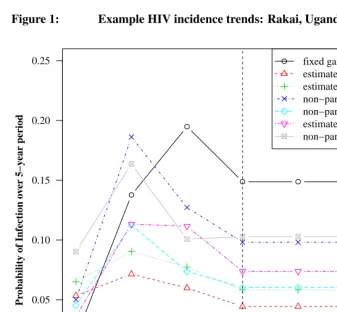
The different trends in HIV incidence used with the HCCMPP to forecast HIV prevalence are shown in Figure 1. Each trend in the plot shows the estimated probabilities of infection over a five-year period for the reference group in Rakai, Uganda (only the posterior means are shown for the estimated trends). For the models where the incidence trend is the same for women and men, only the estimated probabilities for women aged 25-29 are shown.10 In our specifications where the trend is sex-specific, separate trends are shown in the plot corresponding to the sex-specific reference group aged 25-29. The vertical line indicates the last period for which we use data to estimate the model parameters. HIV incidence is assumed to stabilize during this time period, 15–19 years into the epidemic, and the corresponding level of incidence is used to forecast subsequent levels of HIV prevalence. The most striking feature in Figure 1 is how the trend from the fixed gamma curve, which was used in the original analysis (Heuveline 2003), reaches a level that is much higher than the estimated trends during the period 15–19 years into the epidemic. Con-versely, when the trend in HIV incidence is estimated, the level of incidence is higher during the initial period of the epidemic and the peak occurs earlier than the trend from the fixed gamma curve. A second finding is that when separate curves are estimated for men and women, the trends appear to be different, for both the gamma and non-parametric specifications. Among those aged 25–29, estimated incidence based on the non-parametric trend is higher for men during the first five years of the epidemic, with a cross-over in the subsequent projection period, and convergence during the period 15–19 years into the epidemic. This cross-over of the incidence trends for men and women is consistent with the HIV-1 hypothesis described by Gregson et al. (1997), which posits a pattern of HIV transmission in rural areas where men are typically infected first, perhaps while working in an urban center or town, and then infect their female partners at a later point in time. The sex-specific trends estimated using gamma curves, however, suggest that the trend for men and women follow the same pattern and that only the levels are different. A final note is that these differences and cross-overs are only suggestive since there is uncertainty around the point estimates shown in Figure 1.
10In the models where a single HIV incidence trend is used, the shape of the curve will be exactly the same for
Figure 1: Example HIV incidence trends: Rakai, Uganda
●
●
●
● ● ● ●
0.00 0.05 0.10 0.15 0.20 0.25
Years into the Epidemic
Pr
obability of Infection o
v
er 5−y
ear period
0−4 yrs 5−9 yrs 10−14 yrs 15−19 yrs 20−24 yrs 25−29 yrs 30−34 yrs
Estimation Forecast
● fixed gamma
estimated gamma estimated gamma − women non−parametric − women non−parametric
estimated gamma − men non−parametric − men
Notes: The level of incidence corresponds to the sex-specific age group 25-29 years when separate trends are used for women and men, and for women aged 25-29 years when a single trend is used for both groups. Values to the left of the vertical line are used to estimate the HCCMPP parameters, and values to the right are used to make forecasts to compare with data from the DHS surveys.
of Figure 2, show that the risk of infection increases significantly from the 15–19 age group to the 20–24 age group, with the latter experiencing the highest level of incidence. The risk of infection then declines until reaching a fairly stable level after age 35. There are also very few differences between the ML and BM estimates for men, shown in the bottom panel of Figure 2. With either approach, the estimated risk of infection for men is relatively low among those aged 15-19 and clearly increases among the next two older age groups. Uncertainty makes it difficult to identify differences in the risk of infection among men between the ages of 25 and 49, but the ML and BM results seem to suggest that men in their fifties experience a lower risk of infection than men aged 25-34. For both women and men, the ML and BM intervals around the point estimates increase with age, which is expected given the increasingly smaller number of observations at older ages.
Bayesian melding (BM) has been used in previous analyses involving deterministic models of population dynamics and HIV/AIDS that include less than five parameter in-puts (Poole and Raftery 2000; Alkema, Raftery, and Clark 2007). A key finding in this paper is the successful implementation of BM in a relatively high dimensional parameter space using the incremental mixture importance sampling (IMIS) algorithm introduced by Raftery and Bao (2010). We are able to perform statistical inference and to make prob-abilistic projections using models that range from the simplest with 29 parameters up to the most complicated with 36 parameters. The IMIS algorithm proved to be much more efficient than the sampling importance resampling (SIR) technique (Rubin 1987, 1988) that has been used in previous work to implement BM (e.g., Poole and Raftery 2000; Alkema, Raftery, and Clark 2007).11
11Posterior samples of size 3,000 typically include less than 100 unique points when SIR is used to implement
Figure 2: Estimated age schedules of HIV incidence
0.0 0.5 1.0 1.5
Age Group
Ratio to W
omen Aged 25−29
a. Women
15−19 20−24 25−29 30−34 35−39 40−44 45−49 50−54 55−59
● ●
●
●
● ●
● ● ●
● Maximum Likelihood Estimate
Bayesian Melding Estimate
0.0 0.5 1.0 1.5
Age Group
Ratio to W
omen Aged 25−29
b. Men
15−19 20−24 25−29 30−34 35−39 40−44 45−49 50−54 55−59
● ●
● ●
● ●
● ●
●
4.2 Model fit
Having been able to successfully implement BM with various specifications of the model, we are left with the task of choosing among the different models that are distinguished by the trend in HIV incidence. Palloni (1996) pointed out that in a demographic model with HIV/AIDS the force of infection that produces the current level of prevalence should depend on the past level of prevalence, and thus the trend in HIV incidence is endogenous. To make this problem tractable with HCCMPP, Heuveline (2003) assumes an incidence trend based on a gamma curve, a strategy also used in previous models of HIV/AIDS epidemics (e.g., Chin and Lwanga 1991; Salomon and Murray 2001), and treats it as a fixed model input. While the gamma curve may yield a plausible trend, there is at least some uncertainty around this part of the model. In our analysis, we relax the assumption of a fixed gamma curve by estimating the trend in HIV incidence and allowing it to vary by sex and in functional form (see Section 3 for more details about the implementation and estimation). The estimated trends are discussed in the previous section, and here we focus on the comparison of the following five models included in the analysis: (i) fixed gamma curve, (ii) estimated gamma curve, (iii) sex-specific estimated gamma curves, (iv) non-parametric curve, and (v) sex-specific non-non-parametric curves. Given the seemingly large differences between the trends shown in Figure 1, it is natural to be concerned with the relative merit of each model. One standard criterion is how closely each model fits the data. A simple metric for assessing model fit is the sum of squared residuals. According to this measure, there are only slight differences across all of the models with the values ranging from a high of 0.225 for the HCCMPP with the fixed gamma curve to a low of 0.201 for the model with the sex-specific non-parametric trends. An alternative measure for comparing models is Bayes factor (Jeffreys 1939; Kass and Raftery 1995), which is easily calculated from the IMIS approach taken here (Raftery and Bao 2010). The model comparisons based on Bayes factor, with equal prior probabilities given to each model, favor the HCCMPP with the fixed gamma curve over all of the other models, but the evidence is fairly weak since all of the values for the Bayes factors are less than 1.1 – generally, values greater than 3 indicate important differences between the models being compared (Raftery 1995). Although the evidence is weak, it is interesting to note that the Bayesian model comparison favors the simplest model with the fixed gamma curve, which is also the model that is the best at predicting future observations – another important criterion for evaluating the relative merit of different models.
4.3 Model validation: Calibration and predictive performance for Tanzania
Tan-zania, Uganda and Burundi in the mid 1990s. There was little change in the prevalence of HIV in Tanzania from the mid 1990s until the mid 2000s (Asamoah-Odei, Calleja, and Boerma 2004; UNAIDS 2009a), and consequently, if we use our estimated parameter values from the mid 1990s, we should be able to forecast the sex-age distribution of HIV prevalence in the mid 2000s accurately and with reasonable confidence.
Sex-age-specific HIV prevalence measured by the HIV/AIDS Indicator and Demo-graphic and Health Surveys in Tanzania in 2004 and 2007 serve as the targets for our forecast. To produce the forecast we use the best-fitting fixed gamma trend in overall HIV incidence (see Figure 1 for the gamma trends in HIV incidence) and hold it con-stant from year fifteen of each projection (roughly the year 2000 in calendar time). We use our estimated distributions of HIV incidence by sex and age with no modifications for the duration of the forecast. The distribution of forecasted values of HIV prevalence is generated by making multiple draws from the estimated joint parameter distribution and projecting the population forward for each of those with a constant overall incidence trend; see Figure 1. The result is a sex-age-specific distribution of HIV prevalence val-ues at various times in the 2000s that we can use to compare with the empirical valval-ues measured by the surveys.
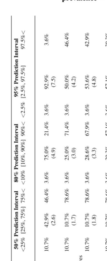
To assess the accuracy and calibration of the forecast, we take the predicted distri-butions for sex-age-specific HIV prevalence for Tanzania12and calculate the quantiles of the 50%, 80%, and 95% credible intervals and compare these to the corresponding ob-servations from the HIV/AIDS Indicator and Demographic and Health Surveys. Table 1 displays these ‘coverage’ results. There is one row for each of the overall HIV incidence trends that we tried and three sets of columns for the 50%, 80% and 95% credible inter-vals. Each of these contains the percent of the empirical observations that fall below the lower limit, within the central interval and above the upper limit. Reading the first row of the table, we find that 11% of the observations fall below the25thpercentile, 43% fall
between the25thand75thpercentiles and 46% above the75thpercentile, etc.
The forecast using the fixed gamma for the overall trend in HIV incidence clearly pro-duces the best calibrated results (the observed coverage comes closest to what we expect), and the calibration is acceptable. 92.9% of observations fall within the 95% credible in-terval with an even 3.6% below and above. Calibration deteriorates slightly as the credible intervals shrink, and there is a slight tendency to understate prevalence, as indicated by the fact that more observations fall above the prediction intervals than expected. Alto-gether the calibration results for Tanzania indicate that the model is reasonably accurate and represents uncertainty in a way that corresponds to empirical observation.
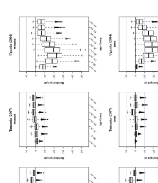
Figure 3 displays the the forecast errors for Tanzania 2004 and 2007 and Uganda
12These predicted distributions are specific to the years when the AIDS Indicator and Demographic and Health
2004, again using the best-fit fixed gamma trend in overall HIV prevalence with a con-stant value for years after 2000. Each plot contains the distribution of forecast errors by age group summarized with a boxplot. If the forecasts were well-calibrated these boxplots would describe compact distributions centered at zero. Each forecast error is the residual between the observed and forecast values (observed – forecast). The distributions arise because there is a distribution of predicted values for each sex-age category. Our fore-casts take into account uncertainty in HIV incidence but not underlying vital rates, and consequently we expect that uncertainty will be slightly underestimated.
Tanzania. Our earlier assessment suggests that the forecasts of the observed levels of
HIV prevalence in Tanzania are reasonable. This is reflected in the left two columns of plots in Figure 3, in which the boxplot for every age group is centered near zero with comparatively short tails. The only systematic deviations from zero are in the age range 30–44 for women and ages 40–44 (2004) and 35–39 (2007) for men. For those ages the forecast appears to be slightly too low. Overall the forecast errors for Tanzania are small – a few percentage points – and the error distributions contain small variation and are centered close to zero.
Uganda.The forecast errors for Uganda (rightmost column of plots in Figure 3) clearly
Figure 3: HIV prevalence forecast error distributions ● ●● ● ●●● ● ●●●● ●●● ● ●●● ● ● ●●●●●●●●●● ● ●●●●● ●●● ● ●● ● ● ●●● ● ●● ●● ● ●● ●● ●● ●●●●●●●● ● ●● ● ● ●● ●● ● ● ●●●● ● ●●●● ●● ●●●●●● ● ● ●● ●●●●●●●●●● ●●●●●●●● ● ● ● ● ●●●●●●● ● ●●● ● ● ●● ●●●● ● ● ● ●●●● ●● ●●●●● ● ●● ● ●● ●●●●● ●●●●●●●●●● ●●● ●●●● ● ● ●● ● ●●● ● ● ● ● ●●●● ● ● ●●● ●●● ● ●●●●●●●● ● ●● ● ●●●●● ● ●●● ●●● ● ●●●● ●●●● ●●●●●● ●●●●● ● ● ●● ● ●●●● ● ● ●● ● ● ●● ● ●●●●● ● ● ● ●● ●●● ● ● ● ● ●● ● ● ●● ● ● ●●● ●● ●● ●● ●● ●●● ●● ● ● ●●●● ● ●●●●●●●●●●●●●●●●● ● ●● ● ●● ●● ●● ● ●●●●●● ●●●● ●●●●●● ● ●●● ●● ●● ●● ●●●● ●●●●●● ● ● ● ● ● ● ●●●●●● ● ●●●● ● ● ● ●●● ● ● ●● ●● ●● ● ●●● ● ● ●● ●● ●●●●● ●●● ● ●● ● −50 −40 −30 −20 −10 0 10 T anzania (2004) w omen Age Gr oup
Residual (pct pt)
15−19 20−4 25−29 30−34 35−39 40−44 45−49 ● ●● ● ●●● ● ●● ●● ● ● ●●● ●● ● ● ● ●●●●●●● ●●● ●● ●●●● ●●● ●● ● ●●●●●● ●●●●●●●●●● ● ●●●●●●●●● ● ● ● ●● ● ●● ● ● ●●●● ● ●●●● ●● ● ● ●●●● ● ● ●● ●●●●● ●●●●●●●●● ●●●● ● ● ● ● ● ●●●● ●●● ● ● ● ●● ● ● ● ● ● ●●● ● ● ●● ●● ●●●●●●● ● ●●● ● ●● ●●●●●●●●●●●●●● ●●● ● ●● ●●●●●●●● ●●● ● ●●●●●● ● ●●●● ●● ●●● ● ●● ●●●●●●● ●●●●●●●●●●●●●●● ● ●●●●●●●● ●●● ● ●●● ●● ●● ●●● ● ●●●●●●●● ●●● ●●● ●●●●● ● ●●● ●●●●●● ● ● ●●● ● ● ●● ● ● ●●● ●● ●● ●● ●● ●● ● ●●● ● ●●● ● ●●●●●●●●●●●●●●●●● ● ●●● ●● ●● ●● ● ●● ● ●●●●●● ●●●●●● ● ●●●● ●●●●●●●● ● ●●●● ●●●● ●● ● ●●●● ●●●● ●●● ● ● ● ●●● ●● ●● ●●●● ● ●●●● ●●●●●●● ● ●●●●●●● ● −50 −40 −30 −20 −10 0 10 T anzania (2007) w omen Age Gr oup
Residual (pct pt)
15−19 20−4 25−29 30−34 35−39 40−44 45−49 ●●●● ●● ● ●●●● ● ● ● ● ● ● ● ● ● ● ●● ● ● ● ●● ●●●●●●● ●●●●● ● ● ● ●●●●●●●●● ● ●●●● ● ●●●●●●●●●●●●●● ●● ● ● ● ●● ● ●● ●● ●● ● ●● ● ●● ●●●●● ●●●●●● ●●●● ●● −50 −40 −30 −20 −10 0 10 Uganda (2004) w omen Age Gr oup
Residual (pct pt)
15−19 20−4 25−29 30−34 35−39 40−44 45−49 50−54 55−59 ●●●● ● ●● ●●● ●●●●●●●●●●●●●●●●●●●●●●●●● ●●● ● ●●●●●●●●●●● ●●●●●●●●●●●●●●●● ●●●●●● ●●●●●●●●●●●●●●●●●●●●●●● ● ● ● ● ●● ● ●●● ●● ●●● ● ● ● ● ● ● ● ●● ●●●●●● ●●● ●● ●●●●● ●● ● ● ●● ●●●● ● ● ●● ● ● ●● ●● ●● ● ● ● ● ●● ●● ●●● ● ●● ● ● ●● ●● ● ● ●●●●● ●●● ●● ● ●●● ●●●●●●●● ● ● ●● ● ● ● ● ●● ● ●● ●●●●●● ● ●●●●● ● ● ● ●●● ●●● ● ● ●● ● ●● ●● ●●●● ●●●●●● ● ● ●● ● ●●●●●●●●●●● ●●●● ●●●● ●● ●●●●● ●● ● ● ● ● ● ● ● ● ●● ● ●● ●●● ●●●● ●●●●●● ●●● ●●● ●●● ●●●●●● ● ●●●●●● ● ● ●●● ●●● ● ●●● ● ● ●●● ●●●● ●●● ●● ●● ●●●● ● ●● ● ●● ●●●● ●●●● ● ● ● ●●● −50 −40 −30 −20 −10 0 10 T anzania (2004) men Age Gr oup
Residual (pct pt)
15−19 20−4 25−29 30−34 35−39 40−44 45−49 ●●● ● ●● ●●● ●●●●●●●●●●●●●●●●●●●● ●●● ●●●●●●●●●●● ●●●●●●●●●●●●●●●● ● ●●●● ●●●●●●●●●●●●●●●●●●●●●● ● ● ● ● ●● ● ●●● ● ●● ●● ● ● ● ● ● ● ● ●●● ●●●● ●● ●●●●●●● ●● ● ●● ●● ●●●●● ● ●●● ● ●● ●● ●● ● ●● ● ● ● ● ●● ●● ●● ● ●● ● ● ●● ●● ●● ●●● ● ● ●● ●●●●●●● ●●● ●●●●●●● ● ● ● ● ● ● ● ● ●●● ●●●●● ● ●● ●●●● ●● ● ● ●● ●●● ● ● ●● ● ●● ●● ●●● ●●● ●●●● ● ●●●●●● ●●●●●● ●●●●●● ●● ●●● ●● ● ●● ●●● ● ● ● ● ●●● ●●● ● ● ● ●● ●● ●●●●●●●●●●● ●● ● ●●● ●●●● ● ●● ●●●●●● ● ● ●●● ●●●●● ● ●● ● ● ●●●●● ● ●●●●●● ●● ●●●●●●● ●●●● ●●●● ●●●● ● ● ●● ●● −50 −40 −30 −20 −10 0 10 T anzania (2007) men Age Gr oup
Residual (pct pt)
15−19 20−4 25−29 30−34 35−39 40−44 45−49 ●● ●● ● ●●●● ● ● ●●● ●● ●●●●●● ● ●● ● ● ● ●● ● ●●● ● ● ●● ●● ● ● ● ●●● ●●●●●●● ●●●● ●●●●● ● ● ●●● ● ●●●●●● ● ● ● ● ●●● ● ● ● ● ● ● ●● ● ● ●●● ●●●●● ●● ●●● ● ● ●●●●● ● ●●● ●●●●●● ●●● ● ●●●●●●●●● ●●● ●● ●●● ● ● ● ●●● ●●● ●● ●● ●●●●● ● −50 −40 −30 −20 −10 0 10 Uganda (2004) men Age Gr oup
Residual (pct pt)
For Ugandan men the situation is similar, but the magnitude of the errors is slightly less and the age-pattern is different. The trough for men is wider covering about ages 30– 44, but not quite as low, reaching a minimum of approximately –19%. The trough also begins to develop at older ages, only showing strong deviation from zero in the 20–24 age group. Similar to women, the99thpercentile of the error distributions does not include
zero until age 35. The age-pattern of deviations in the male errors indicate a reduction in incidence over a broad range of ages from roughly 20–29 to 40–49, with the largest reductions over roughly ages 20–44.
4.4 Conclusions
Using some of the early measures of HIV prevalence from community-based studies in Tanzania, Uganda and Burundi during the early to mid 1990s, we estimate the age profile of HIV incidence that is consistent with underlying vital rates and the observed age pattern of HIV prevalence. We apply the new Bayesian melding with IMIS estimation procedure to ‘fit’ the HIV enabled cohort component model of population projection created by Heuveline (2003). Our results corroborate both his and our own earlier work using a maximum likelihood estimation procedure. The age profile of incidence is younger and more focused for women with peaks in the 20-24 year age group for women and 25-29 year age group for men.
The Bayesian estimation framework provides an advantage compared to maximum likelihood techniques because it enables us to quantify uncertainty in estimated parame-ter values in a statistically valid way that can be inparame-terpreted and manipulated in a fully probabilistic framework. Most important to us, however, is the opportunity to produce probabilistic projections – true forecasts – of the HIV-affected populations. This allows us to validate our model in one more way by comparing (probabilistic) forecasts of HIV prevalence with empirical measures of prevalence in Tanzania. There was little change in HIV incidence in Tanzania between the mid 1990s and early 2000s, and we are able to predict, with reasonably calibrated accuracy, age-specific HIV prevalence in Tanzania in the early 2000s by forecasting forward with no change in our estimated HIV incidence pattern.
We use one further advantage of the Bayesian framework to compare models with different specifications of the trend in HIV incidence. The Bayesian framework allows us to use Bayes factors to compare the models and determine that the simple fixed gamma curve originally specified by Heuveline produces better forecasts compared to a variety of more flexible specifications with more parameters – the Bayes factor takes into ac-count the number of parameters, effectively penalizing models with larger numbers of parameters (degrees of freedom).
the age-pattern of reductions in prevalence resulting from the well-documented declines in HIV incidence that took place in Uganda between the early 1990s and mid 2000s. This age pattern of change in HIV prevalence reflects the earlier and younger changes in HIV incidence that were required to reduce the HIV+ fraction of the population.
5.
Discussion
5.1 Summary
This paper makes two main contributions, the first is to validate the HCCMPP developed by Heuveline (2003). We find that the model can produce accurate forecasts of age- and sex-specific HIV prevalence in Tanzania, and that an assumption of a stabilized trend in HIV incidence provides estimates of the extent of the decline in the risk of HIV infection in Uganda. In order to produce accurate forecasts with the HCCMPP for other countries in sub-Saharan Africa, the model may require new modifications to capture the geographic heterogeneity in the HIV epidemics across this region. Other potential sources of vari-ability not captured by the model are the uncertainty around the start date of the epidemic and around vital rates. Including these as estimated model inputs may be useful in terms of improving the predictive performance of HCCMPP and applying it to other countries. Despite these issues, it is impressive how well the model does when considering the dif-ferences between the data used to calibrate it (i.e. estimate the HCCMPP parameters) and the data used to validate the model forecasts. The former were collected from relatively small community-based studies while the latter were collected from nationally represen-tative samples.
The second contribution is to use a new Bayesian estimation technique designed for deterministic models. We have shown that the IMIS algorithm (Raftery and Bao 2010) can be used successfully to implement the Bayesian melding estimation approach with the 30+ parameter HCCMPP model. This suggests that the approach could be used more generally to enable demographers to quantify, in a statistically rigorous way, the uncertainty around both parameter estimates and model outputs in many of the deterministic models they use. With respect to the CCMPP (HIV-enabled or not), the ability to quantify uncertainty around demographic projections is useful in a fundamental sense. This allows decision-makers to define the probability of extreme outcomes, with respect to the levels of HIV prevalence and incidence, and make informed cost-benefit and risk tolerance decisions in a valid probabilistic framework. Furthermore, probabilistic projections produced using a CCMPP-type model and Bayesian melding with IMIS can be used to validate the model by comparing forecasts to observed values. The Bayesian framework can also be used to compare competing model specifications using Bayes factors.
they mature by using data to estimate the trends in HIV incidence. Our results suggest that the gamma curve used by Heuveline (2003) in the original work with HCCMPP provides the best predictive performance of sex-age-specific HIV prevalence in Tanzania.
5.2 Recommendations
1. Because HIV incidence is such an important indicator of an HIV epidemic, and because it is so difficult to measure HIV incidence empirically, epidemiologists, demographers and statisticians should prioritize further development of mathemat-ical models and statistmathemat-ical procedures that allow us to estimate HIV incidence with uncertainty. To be of practical use to decision makers in the small areas where interventions are implemented and evaluated, these techniques should attempt to provide estimates of incidence by time, sex and age.
2. Given the success of Bayesian melding with IMIS applied to the 30+ parameter HCCMPP and the inherent advantages of the Bayesian framework, epidemiologists and demographers should consider applying this and similar procedures to other models and estimation procedures common to their disciplines.
3. We have successfully produced probabilistic forecasts of HIV epidemics taking into account uncertainty in HIV incidence. Using a similar Bayesian framework, future work on both HCCMPP and regular non-HIV CCMPP should incorporate uncertainty in vital rates and migration to produce probabilistic forecasts that take into account all major sources of uncertainty.
4. The Bayesian framework gives us the ability to conduct Bayesian model compar-ison using Bayes factors. This ability should be used to investigate the effects of interventions by comparing models that do and do not model the intervention. Bayesian model comparison will tell us if the intervention model fits the data bet-ter than the non-inbet-tervention model, and if so, the paramebet-ter estimates and model outputs will tell us what the effects are and how effective the intervention is.
5.3 Ideas for future work
pop-ulation, this share of the infected population should experience improved survival and fertility prospects, and a diminished likelihood of infecting others, relative to those who are HIV+ but not receiving ART. Additional modifications could include the ability to model potential interventions related to male circumcision and microbicides (McNeil Jr. 2010). Building in these features would make the HCCMPP more realistic, and poten-tially improve the model’s prospects for successfully monitoring and forecasting HIV epidemics. However, in order to add these new features, the overall model would have to be made simpler to require fewer parameters, in order to ensure that the whole thing remains identifiable and tractable enough to estimate. This could be done by modeling existing parameters and defining (a smaller number of) new hyper parameters to govern those models and/or by collapsing across age groups in which there is little meaningful variation.
6.
Attributions & acknowledgements
Jason R. Thomas conducted the bulk of the analysis for this project, wrote and ran all of theRcode and wrote the first draft of the manuscript. Samuel Clark conceived and supervised this project and wrote the final manuscript. With Adrian Raftery, Le Bao refined the IMIS method and wrote the original IMIS code that was adapted for use in this project, and Le Bao contributed significantly to the adaptation of his IMIS code for use in this project. All authors have read and approved this manuscript.
This project was supported by a seed grant from the Center for Statistics and the Social Sciences (CSSS), University of Washington and by grants K01 HD057246, R01 HD054511, and R24 HD047873 from the National Institute of Child Health and Human Development (NICHD) of the National Institutes of Health (NIH), as well as grant num-bers T32 AG00129 and P30 AG17266 from the National Institute of Aging. The content of the work presented here is solely the responsibility of the authors and does not neces-sarily represent the official views of the the NIH. The authors are very grateful to Patrick Heuveline for his correspondence and for making his work available. We also thank Adrian Raftery, Leontine Alkema, Jennifer Chunn, Greg Mathews, David Sharrow, and Mark Wheldon for invaluable discussion during the preparation of this work. The second author would also like to thank colleagues at the Africa Centre for Health and Popula-tion Studies, University of KwaZulu-Natal, South Africa for their hospitality and useful comments on an early version of this work.
References
Alkema, L., Raftery, A.E., and Clark, S.J. (2007). Probabilistic Projections of HIV prevalence using Bayesian Melding. Annals of Applied Statistics 1(1): 229–248. doi:10.1214/07-AOAS111.
Anderson, R.M. (1988). The role of mathematical models in the study of HIV transmis-sion and the epidemiology of AIDS. JAIDS Journal of Acquired Immune Deficiency Syndromes1(3): 241–256.
Asamoah-Odei, E., Calleja, J.M.G., and Boerma, J.T. (2004). HIV prevalence and trends in sub-Saharan Africa: No decline and large subregional differences. The Lancet
364(9428): 35–40. doi:10.1016/S0140-6736(04)16587-2.
Bongaarts, J., Buettner, T., Heilig, G., and Pelletier, F. (2008). Has the HIV epidemic peaked? Population and Development Review34(2): 199–244. doi:10.1111/j.1728-4457.2008.00217.x.
Bowley, A.L. (1924). Births and population in Great Britain.Economic Journal34(134): 188–192.doi:10.2307/2223159.
Cannan, E. (1895). The probability of a cessation of the growth of population in England and Wales during the next century. Economic Journal 5(20): 505–515. doi:10.2307/2956626.
Cassels, S., Clark, S.J., and Morris, M. (2008). Mathematical models for HIV transmission dynamics: Tools for social and behavioral science re-search. JAIDS Journal of Acquired Immune Deficiency Syndromes 47: 34–39. doi:10.1097/QAI.0b013e3181605da3.
Chin, J. and Lwanga, S.K. (1991). Estimation and projection of adult AIDS cases: A simple epidemiological model.Bulletin of the World Health Organization69(4): 399– 406.
Granich, R.M., Gilks, C.F., Dye, C., De Cock, K.M., and Williams, B.G. (2009). Uni-versal voluntary HIV testing with immediate antiretroviral therapy as a strategy for elimination of HIV transmission: A mathematical model. The Lancet373(9657): 48– 57.doi:10.1016/S0140-6736(08)61697-9.
Grassly, N.C., Morgan, M., Walker, N., Garnett, G., Stanecki, K.A., Stover, J., Brown, T., and Ghys, P.D. (2004). Uncertainty in estimates of HIV/AIDS: The estimation and application of plausibility bounds.Sexually Transmitted Infections80(1): i31–i38. doi:10.1136/sti.2004.010637.
Gregson, S., Anderson, R.M., Ndlovu, J., Zhuwau, T., and Chandiwana, S.K. (1997). Recent upturn in mortality in rural Zimbabwe: Evidence for an early demographic impact of HIV-1 infection.AIDS11(10): 1269–1280.
Hallett, T.B., Aberle-Grasse, J., Bello, G., Boulos, L.M., Cayemittes, M.P.A., Cheluget, B., Chipeta, J., Dorrington, R., Dube, S., Ekra, A.K., Garcia-Calleja, J.M., Garnett, G.P., Greby, S., Gregson, S., Grove, J.T., Hader, S., Hanson, J., Hladik, W., Ismail, S., Kassim, S., Kirungi, W., Kouassi, L., Mahomva, A., Marum, L., Maurice, C., Nolan, M., Rehle, T., Stover, J., and Walker, N. (2006). Declines in HIV preva-lence can be associated with changing sexual behaviour in Uganda, urban Kenya, Zimbabwe, and urban Haiti. Sexually Transmitted Infections 82(suppl 1): i1–i18. doi:10.1136/sti.2005.016014.
Hallett, T.B., Singh, K., Smith, J.A., White, R.G., Abu-Raddad, L.J., and Garnett, G.P. (2008). Understanding the impact of male circumcision interventions on the spread of HIV in southern Africa.PLoS One3(5): e2212. doi:10.1371/journal.pone.0002212. Hallett, T.B., White, P.J., and Garnett, G.P. (2007). Appropriate evaluation of HIV
preven-tion intervenpreven-tions: From experiment to full-scale implementapreven-tion.Sexually transmitted infections83(suppl 1): i55–i60.doi:10.1136/sti.2006.023663.
Hallett, T., ˙Zaba, B., Todd, J., Lopman, B., Mwita, W., Biraro, S., Gregson, S., Boerma, J., on behalf of the ALPHA Network. (2008). Estimating incidence from preva-lence in generalised HIV epidemics: Methods and validation. PLoS Med 5(4): e80. doi:10.1371/journal.pmed.0050080.
Hesterberg, T. (1995). Weighted average importance sampling and defensive mixture distributions.Technometrics37(2): 185–194. doi:10.2307/1269620.
Heuveline, P. (2003). HIV and population dynamics: A general model and maximum-likelihood standards for East Africa. Demography 40(2): 217–245. doi:10.1353/dem.2003.0013.
Kamali, A., Carpenter, L.M., Whitworth, J.A.G., Pool, R., Ruberantwari, A., and Ojwiya, A. (2000). Seven-year trends in HIV-1 infection rates, and changes in sexual beav-iour, among adults in rural Uganda. AIDS14(4): 427–434. doi:10.1097/00002030-200003100-00017.
Kass, R.E. and Raftery, A.E. (1995). Bayes factors. Journal of the American Statistical Association90(430): 773–795.doi:10.2307/2291091.
Keyfitz, N. and Caswell, H. (2005). Applied Mathematical Demograph. New York: Springer, third edition ed.
Leslie, P.H. (1945). On the use of matrices in certain population mathematics.Biometrika
33(3): 183–212. doi:10.2307/2332297.
Mbulaiteye, S.M., Mahe, C., Whitworth, J.A.G., Ruberantwari, A., Nakiyingi, J.S., Ojwiya, A., and Kamali, A. (2002). Declining HIV-1 incidence and associated preva-lence over 10 years in a rural population in south-west Uganda: A cohort study. The Lancet360: 41–46.doi:10.1016/S0140-6736(02)09331-5.
McDougal, J.S., Parekh, B.S., Peterson, M.L., Branson, B.M., Dobbs, T., Ackers, M., and Gurwith, M. (2006). Comparison of HIV type 1 incidence observed during longitudinal follow-up with incidence estimated by cross-sectional analysis using the BED capture enzyme immunoassay. AIDS Research and Human Retroviruses 22(10): 945–952. doi:10.1089/aid.2006.22.945.
McNeil Jr., D.G. (2010). African studies give women hope in HIV fight.New York Times
(July 19).
McWalter, T.A. and Welte, A. (2009). A comparison of biomarker based incidence esti-mators. PLoS One4(10): e7368.doi:10.1371/journal.pone.0007368.
McWalter, T.A. and Welte, A. (2010). Relating recent infection prevalence to incidence with a sub-population of assay non-progressors. Journal of mathematical biology
60(5): 687–710. doi:10.1007/s00285-009-0282-7.
Palloni, A. (1996). The demography of HIV/AIDS. Population Index62(4): 601–652. doi:10.2307/3646371.
Parekh, B.S., Kennedy, M.S., Dobbs, T., Pau, C.P., Byers, R., Green, T., Hu, D.J., Vanich-seni, S., Young, N.L., Choopanya, K., Mastro, T.D., and McDougal, J.S. (2004). Quan-titative detection of increasing HIV type 1 antibodies after seroconversion: A simple assay for detecting recent HIV infection and estimating incidence.AIDS Research and Human Retroviruses18(4): 295–307.doi:10.1089/088922202753472874.
Pearl, R. and Reed, L.J. (1920). On the rate of growth of the population of the United States since 1790 and its mathematical representation. Proceedings of the National Academy of Science6(6): 275–288.doi:10.1073/pnas.6.6.275.
Poole, D. and Raftery, A.E. (2000). Inference for deterministic simulation models: The Bayesian Melding approach.Journal of the American Statistical Association95(452): 1244–1255.doi:10.2307/2669764.
Pritchett, H.S. (1891). A formula for predicting the population of the United States. Publi-cations of the American Statistical Association2(14): 278–286.doi:10.2307/2276575. R Foundation for Statistical Computing (2010). The R Project for Statistical Comput-ing. [electronic resource]. R Foundation for Statistical ComputComput-ing. Http://www.R-project.org.
Raftery, A.E. (1995). Bayesian model selection in social research.Sociological Method-ology25: 111–163.doi:10.2307/271063.
Raftery, A.E. and Bao, L. (2010). Estimating and projecting trends in HIV/AIDS gen-eralized epidemics using incremental mixture importance sampling.Biometrics66(4): 1162–1173.doi:10.1111/j.1541-0420.2010.01399.x.
Rubin, D.B. (1988). Using the sir algorithm to simulate posterior distributions. In: Bernardo, J., Degroot, D., Degroot, M., Lindley, D., and Smith, A. (eds.).Bayesian Statistics 3. Oxford: Oxford University Press: 395–402.
Rubin, D.B. (1987). A noniterative sampling/importance resampling alternative to the data augmentation algorithm for creating a few imputation when fractions of missing information are modest: The SIR algorithm.Journal of the American Statistical Asso-ciation82(398): 543–546.doi:10.2307/2289460.
Salomon, J.A. and Murray, C.J.L. (2001). Modelling HIV/AIDS epidemics in sub-Saharan Africa using seroprevalence data from antenatal clinics.Bulletin of the World Health Organization79(7): 596–607.