University of New Orleans University of New Orleans
ScholarWorks@UNO
ScholarWorks@UNO
University of New Orleans Theses and
Dissertations Dissertations and Theses
5-22-2006
Reducing the Hot Spot Effect in Wireless Sensor Networks with
Reducing the Hot Spot Effect in Wireless Sensor Networks with
the Use of Mobile Data Sink
the Use of Mobile Data Sink
Yacine Chikhi
University of New Orleans
Follow this and additional works at: https://scholarworks.uno.edu/td
Recommended Citation Recommended Citation
Chikhi, Yacine, "Reducing the Hot Spot Effect in Wireless Sensor Networks with the Use of Mobile Data Sink" (2006). University of New Orleans Theses and Dissertations. 365.
https://scholarworks.uno.edu/td/365
REDUCING THE HOT SPOT EFFECT IN WIRELESS SENSOR
NETWORKS WITH THE USE OF MOBILE DATA SINK
A Thesis
Submitted to the Graduate Faculty of the
University of New Orleans
in partial fulfillment of the
requirements for the degree of
Master of Science
in
Computer Science
by
Yacine Chikhi
B.S Pierre & Marie Curie University Paris, 2004
Acknowledgements
I would like to express my appreciation to my advisor, Dr. Jing Deng. I want to sincerely
thank him for his support, constant availability and pertinent advices. He, the first, introduced me
to Wireless Sensor Networks and encouraged me in pursuing this thesis research and I am deeply
grateful for that.
I would also like to thank the two members of my committee: Dr Vassil Roussev and Dr
Yixin Chen. I had the chance to attend classes offered by these excellent teachers and being
exposed to their excellence and their competence in Computer Science makes me feel honored
and flattered to have them on my thesis committee. I must mention their tremendous kindness,
their availability and constant support with their students in general, and myself in particular.
In addition, I would like to thank the rest of the CS faculty members, since I have always been
very satisfied with the level of knowledge and pedagogy offered by the teachers of our
department. A special thanks to Venkata for his eternal availability and smile.
On a personal note, I would like to thank my brother Jalil for always being my model and
source of inspiration and my sister Nedjma and her family for their unconditional love and
support.
Maya, I love you and nothing that I have accomplished or will accomplish is possible without
knowing that you are by my side.
I shall cloture these acknowledgements by thanking the most important person in my life: my
mother Fettouma. This work as well as any other success in my life is dedicated to you. Every
Table of Contents
Table of Figures ... iv
Table of Tables ... iv
Abstract ... v
Chapter I: Introduction... 1
I.1 Background ... 1
I.2 The Hot Spot Effect ... 4
I.3 Thesis Organization... 7
Chapter II: Related Work... 8
Chapter III: Details of the Mobile Data Sink Scheme... 11
III.1 Assumptions ... 11
III.2 Path Establishment for Data Sink Motion... 12
III.3 Cost & Overhead ... 23
Chapter IV: Performance Evaluation... 26
IV.1 Methodology... 26
IV.2 1D Network ... 27
IV.3 2D Network – Assumptions ... 29
IV.4 Results... 31
Chapter V: Conclusion... 41
Chapter VI: Future Work... 42
References... 44
Table of Figures
Figure 1: Data transmission pattern in a Wireless Sensor Network ...12
Figure 2: Importance of sink mobility in breaking the transmission tree structure and relieving the Hot Spot nodes in a simplified network...13
Figure 3: TRV assignment for Hot Spot nodes after time T_obs ...17
Figure 4: Determination of the sink's circular motion around the initial position...19
Figure 5: determination of the position of the mobile sink between two sub-trees...21
Figure 6: Path determination for data sink motion based on TRV of Hot Spot sensors and their geographical positions ...22
Figure 7: Impact of high traffic rate and high node density regions on the optimal data sink position within 1D network ...28
Figure 8: Comparative network lifetimes for fixed sink network and network implementing the Mobile Data Sink scheme with variable node density and data traffic rate...32
Figure 9: Comparative standard variance of traffic rate among nodes for both fixed and mobile data sink schemes...33
Figure 10: Comparative average distribution of energy consumption among network nodes for fixed and mobile data sink schemes...34
Figure 11: Comparative throughputs in standard variance of node traffic rate and network lifetime for Mobile sink and Energy Balanced Propagation schemes ...36
Figure 12: Comparative throughputs in network lifetime and standard variance of node traffic rate for Mobile sink scheme and fixed data sink using the Energy Map scheme...39
Abstract
The Hot Spot effect is an issue that reduces the network lifetime considerably. The network
on the field forms a tree structure in which the sink represents the root and the furthest nodes in
the perimeter represent the leaves. Each node collects information from the environment and
transmits data packets to a “reachable” node towards the sink in a multi-hop fashion. The closest
nodes to the sink not only transmit their own packets but also the packets that they receive from
“lower” nodes and therefore exhaust their energy reserves and die faster than the rest of the
network sensors.
We propose a technique to allow the data sink to identify nodes severely suffering from the
Hot Spot effect and to move beyond these nodes. We will explore the best trajectory that the data
sink should follow. Performance results are presented to support our claim of superiority for our
I Introduction:
I.1 Background:
Recent researches in wireless communications and digital electronics have allowed the
development of low-cost and low-power multifunctional sensor nodes. Those devices are small
in size and communicate in short distances.
The sensors, which role consists of sensing, processing data partially, and communicating
components, leverage the idea of sensor networks based on collaborative effort of a large number
of nodes to collect and process data.
Sensor networks represent a significant improvement over traditional sensors, which are
deployed in the following two ways:
Firstly, sensors can be positioned far from the actual phenomenon, i.e., something known by
sense perception. In this approach, large sensors that use some complex techniques to distinguish
the targets from environmental noise are required.
Secondly, several sensors that perform only sensing can be deployed. The positions of the
sensors and communications topology are carefully engineered. They transmit time series of the
sensed phenomenon to the central nodes where computations are performed and data are fused.
A sensor network is composed of a large number of sensor nodes, which are densely deployed
either inside the phenomenon or very close to it.
The position of sensor nodes does not need to be engineered or pre-determined. This allows
random deployment in inaccessible terrains or disaster relief operations. Sensors can be literally
dropped within the targeted field. On the other hand, this also means that sensor network
Another unique feature of sensor networks is the cooperative effort of sensor nodes. Sensor
nodes are fitted with an on-board processor. Instead of sending the raw data to the nodes
responsible for the fusion, sensor nodes use their processing abilities to locally carry out simple
computations and transmit only the required and partially processed data.
The above described features ensure a wide range of applications for sensor networks. Some
of the application areas are health, military, and security.
Sensor networks can also be used to detect foreign chemical agents in the air and the water.
They can help to identify the type, concentration, and location of pollutants. In essence, sensor
networks will provide the end user with intelligence and a better understanding of the
environment.
We envision that, in future, wireless sensor networks will be an integral part of our lives,
more so than the present-day personal computers.
Realization of these and other sensor network applications require wireless ad hoc networking
techniques. Although many protocols and algorithms have been proposed for traditional wireless
ad hoc networks, they are not well suited for the unique features and application requirements of
sensor networks. To illustrate this point, the differences between sensor networks and ad hoc
networks are outlined below:
• The number of sensor nodes in a sensor network can be several orders of magnitude higher
than the nodes in an ad hoc network.
• Sensor nodes are densely deployed.
• Sensor nodes are prone to failures.
• Sensor nodes mainly use broadcast communication paradigm whereas most ad hoc networks
are based on point-to-point communications.
• Sensor nodes are limited in power, computational capacities, and memory.
• Sensor nodes may not have global identification (ID) because of the large amount of
overhead and large number of sensors.
Since a large number of sensor nodes are densely deployed, neighbor nodes may be very close
to each other. Hence, multi hop communication in sensor networks is expected to consume less
power than the traditional single hop communication. Furthermore, the transmission power
levels can be kept low, which is highly desired in covert operations.
Multi hop communication can also effectively overcome some of the signal propagation
effects experienced in long-distance wireless communication.
Sensor networks may consist of many different types of sensors such as seismic, low
sampling rate magnetic, thermal, visual, infrared, acoustic and radar, which are able to monitor a
wide variety of ambient conditions that include the following: temperature, humidity, vehicular
movement, lightning condition, pressure, soil makeup, noise levels, the presence or absence of
certain kinds of objects, mechanical stress levels on attached objects, and the current
characteristics such as speed, direction, and size of an object.
Sensor nodes can be used for continuous sensing, event detection, event ID, location sensing,
and local control of actuators. The concept of micro-sensing and wireless connection of these
nodes promises many new application areas. We categorize the applications into military,
environment, health, home and other commercial areas. It is possible to expand this classification
One of the most important constraints on sensor nodes is the low power consumption
requirement.
Sensor nodes carry limited, generally irreplaceable, power sources. Therefore, while
traditional networks aim to achieve high quality of service provisions, sensor network protocols
must focus primarily on power conservation. They must have inbuilt trade-off mechanisms that
give the end user the option of prolonging network lifetime at the cost of lower throughput or
higher transmission delay.
I.2 The Hot Spot Effect:
Many researchers are currently engaged in developing schemes that fulfill these requirements.
Actually, most of the latest studies mainly focus on different algorithms, transmission
protocols and aggregation techniques to save power and extend the network lifetime.
This work falls under the same purpose, treating specifically a critical aspect of a multi-hop
network lifetime: the Hot Spot effect.
The Hot Spot effect is a major issue affecting network lifetime, often causing the collapse of
the system when there are still energy resources within a large group of its nodes.
The network topology varies depending on the purpose it serves and the field dispositions it
needs to adapt to. Sometimes many data sinks are needed to collect information from sensors that
are widely spread, but most wireless sensor networks are composed of sensing nodes and a
unique, fixed, central data sink that collects the information from those nodes in a multi-hop
transmission fashion.
The Hot Spot effect is created by the traffic pattern established among the network nodes.
Once that node receives those information packets, it forms new packets that include both
received data and information sensed and pre-processed by the node itself. Then, using the same
transmission pattern it transmits to the next node.
Based on this transmission pattern, the closest nodes to the data sink will generally have more
packets to (re)transmit to that sink, and will run out of energy earliest. When these nodes run out
of energy, holes may be created in the network in critical areas of the system: the node layer the
surrounds the sink and forwards network data to it. These holes may lead to collapse of network
functionalities since farther sensors might not be able to transmit to the data sink anymore.
Intermediate sensors are not only needed to sense and process field information but fulfilling
their “router” role is as much crucial.
A major trade-off in a tree-based transmission structure is the uneven energy consumption
among sensors. The Hot Spot nodes (the ones in the Hot Spot region) exhaust their resources
faster and cause the collapse of the system while other, farther nodes might still have enough
energy to sense, process and transmit information. Optimizing the energy consumption
distribution is a major key in extending the network lifetime.
In this work, we try to mitigate the adverse impact of the Hot Spot effect on the network
lifetime. Since this effect is based on the fact that a node has many packets from “lower” nodes
to transmit, we propose a technique to move the data sink in order to reduce the transmission
load of these nodes. Our goal is to balance the energy consumption among nodes to a certain
level and prolong the network lifetime.
Talking about a mobile data sink involves naturally changing the transmission tree structure
In this work, we demonstrate the performance gain of allowing the data sink to move to
certain locations. In that matter it is important to build a realistic 2-D model with a widely used
data transmission scheme. For that model we must determine the optimal lifetime when using a
fixed sink and then apply our scheme for performance evaluation.
The modeling process is first implemented through a simplified D model. Our
1-demensional network is not meant to represent any real-life application but serves the purpose of
modeling the energy consumption pattern and establishing an energy consumption formula, used
throughout this work.
The determination of the optimal fixed sink position is necessary, not only to allow the
estimation of the optimal network lifetime, but to determine the path of our mobile data sink as
well. A general formula to estimate the sink’s optimal position will be presented in this work in
that matter.
In our discussions, we consider several real-world applications: some regions of the network
might have a higher node density than others and that might (should) affect the optimal position
of the sink. Some regions might also collect more information and therefore will have a higher
traffic rate towards the sink, and we shall see that it affects the optimal position of the data sink
as well.
We will demonstrate that the challenges of designing a mobile data sink technique lie in
establishing the path that the data sink shall take and determining the time period that needs to be
spent in each position. Such time spans should be estimated according to the traffic pattern
The sink needs to move towards the regions that have a high traffic rate to relief them from
their load without “neglecting” regions of lower priority. The time span in each region is a key in
determining the degree of assistance that the data sink motion provides to each area.
Plus, the sink should be able to give a “directional importance” to the traffic rate that it
receives, and that should help it to evolve within the network. Data sink being larger devices than
the regular sensors, they might be equipped with a GPS system, allowing them to identify and
transmit their exact position, along with a directional antenna that is used not only to collect
information but also recognize the direction of the transmitting source. With these two important
features, the data sink has a precise knowledge of the traffic pattern surrounding it.
This work proposes a mobile data sink scheme that relieves the Hot Spot nodes from their
transmission load, balances to a certain extent the energy consumption among sensors in order to
extend the network lifetime.
I.3 Thesis Organization:
The remainder of this thesis is structured as follows: in Chapter II, we review the related
work: what has been proposed in a matter of extending the network lifetime in general. We
present our technique and discussions in Chapter III. Performance evaluations are presented in
Chapter IV, stressing the enhancement that a mobile data sink brings compared to a fixed data
sink. In Chapter V, we summarize the work. Finally, Chapter VI proposes ideas, possible future
II Related Work:
Energy saving is a major research topic for Wireless Sensor Networks and many interesting
studies have been proposed over the years to extend those networks’ lifetime. Several latest
studies focused on actual transmission protocols, information aggregation techniques, and
transmission tree restructuring to increase the network lifetime [1,3,5,9]. Nevertheless, the
concept of a mobile data sink has not been widely considered.
The reason is related to the difficulty of controlling a mobile data sink. As mentioned in our
introduction, sensors are often placed in inhospitable environment with geographical topologies
that do not allow easy access to the network devices. We argue that our mobile scheme
determination is computable by a sensor device and therefore doesn’t require any human
assistance while evolving around the studied field.
Nevertheless, few researches based their work on networks with mobile data sinks, although
not stressing the importance of the sink mobility in reducing the Hot Spot Effect.
The SEAD protocol [6] for instance has been established to take advantage of the mobile data
sink technique to reduce the energy consumption while restructuring the transmission tree. It
considers low-density networks with multiple data sinks without taking advantage of those
devices’ motion to reduce the Hot Spot Effect. Instead, it emphasizes efficient transmission path
establishment.
SEAD proves that multiple transmission tree restructuring can be less expensive energy-wise
than direct diffusion and multicast transmission protocols, both very used in Wireless Sensor
the system topology constantly. We will demonstrate that the trade-off of that process confirms
what SEAD indicated in that matter in IV.3.
The relatively short average lifetime of a sensor is a major concern in this type of networks.
Efficient energy-saving dissemination protocols, such as SEAD, are crucial since the
transmission-tree of the system needs to be constantly rebuilt.
Thus, research [5] considers a shortest path transmission scheme that increases significantly
the network lifetime compared to a basic multi-hop transmission scheme with a fixed data sink.
We shall see in Chapter IV that we propose a variant of that multi-hop approach based on an
important assumption: all nodes are informed of the data sink position at all time.
As seen in [5,7,8], the data sink can be a powerful device equipped with a GPS, a directional
transmission/reception antenna and a powerful energy reserve; in our case the data sink is able
to broadcast its position to all its sub-nodes in order for them to forward their packets to it.
Broadcasting packets in a Wireless Sensor network is a common procedure, but our scheme
only requires this operation from the sink.
Research [4] proposes an energy balanced propagation scheme to normalize the consumption
among all nodes, which reduces significantly the Hot Spot effect. The scheme is based on a
probabilistic approach determining if a sensor node should transmit to the next 1-hop away
sensor towards the sink or increase its transmission range instead and transmit directly to the
sink. The decision is made based on the energy level of the transmitting node’s neighbors.
In our performance evaluation, we will compare our scheme’s throughput to the one obtained
Our transmission pattern is based on a multi-hop transmission as it has been assessed in
several other research projects [1,3,10] and is detailed in Chapter IV.
Unlike conventional wireless ad hoc networks, a wireless sensor network potentially
comprises of hundreds to thousands of nodes [8]. The sensors have to operate in noisy
environments and, in order to achieve good sensing resolution, higher densities are required.
Therefore, in a sensor network, scalability and optimal energy usage are crucial factors.
Energy maps have been proposed in that matter. Sensors keep track of the energy level of all
their 1-hop away neighbors and decide what the most appropriate node to transmit to is, based on
that knowledge.
The energy map technique is widely used [11] and allows a considerable network lifetime
extension compared to a “basic” scheme where the sensor only transmits to the closest node in
range towards the sink.
Our scheme uses a hybrid energy-map technique since each sensor has knowledge of the
energy level of all 1-hop away neighbors but transmits to the closest in range towards the sink
persistently until that node fails (see III).
This approach keeps the number of tree restructuring down compared to a regular technique
where each node tries to balance its packet distribution among its neighbors.
We will explore trade-offs between the two energy map variants as well in Chapter IV.
III Details of the Mobile Data Sink scheme:
III.1 Assumptions:
Wireless sensor networks vary in their topology, density, and transmission protocols
depending on the field that they are sensing and the level of data generation that is expected from
them.
We present our assumptions of the network that we studied as followed:
●The number of sensors in a network can easily reach hundreds to thousands. Our work
maintains a reasonable node density within the proposed network: average of 1 node per
meter square.
●Our network relies on a unique data sink to collect data from all sensors in the network.
Transmissions towards the sink are made in a multi-hop fashion unless the data sink is in the
range of the transmitting node;
●Depending on the studied phenomenon, nodes can either generate data when sensing an
important event, or sending updates periodically towards the sink. In this work, every sensor
node generates a fixed rate sensing results and these results need to be delivered to the unique
data sink of the network;
●We assume that the data sink has certain mobility capability while all other nodes are
fixed. In common sensor networks, the sensors might have a very restrained mobility due to
independent field factors, but their mobility is often neglected since it has no effect on the
system transmission structure and the energy dissipation caused by the displacement is
minimal compared to the cost of a single packet transmission. Therefore, we will not consider
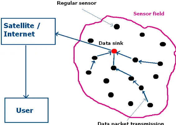
●The data sink is the only device equipped with a GPS and a powerful transmitting
antenna. Therefore, it is responsible for partially processing all sensed data and forwarding it
to a satellite/user for final analysis. Regular sensor nodes only have limited knowledge of the
network. They only have directional information of the location of their 1-hop away
neighbors [8]. They do not use multicast in that matter but node-to-node transmission.
Figure 1: Data transmission pattern in a Wireless Sensor Network
III.2 Path Establishment for Data Sink Motion:
III.2.1 Motivation:
If the sink wants to move and break the tree structure of the network to reduce the Hot Spot
effect, it should pass the position of the overloaded node and sit between its position and the rest
of the lower nodes in that high density region. Nevertheless, doing so will only extend the
The data sink needs to go in a position deep enough within the region itself to change the
sub-tree transmission structure and balance the energy consumption within its nodes.
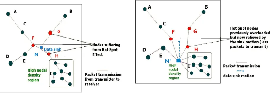
Figure 2 shows an illustration of how the sink’s mobility changes the transmission tree
structure and balances the energy consumption among nodes in a simple network.
Figure 2: Importance of sink mobility in breaking the transmission tree structure and relieving the Hot Spot nodes in a simplified network
Table I illustrates the redistribution of transmission loads among the nodes, before and after
the sink motion. The numbers have been normalized against the traffic rate of each sensor. Here
we assume that all nodes transmit 1 data packet per second. The load is then given in packets
received from lower nodes per second plus one packet transmitted by the node itself.
Nodes A B C D E F G H I
Load before motion 1 1 2 1 2 5 2 9 2
Load after motion 1 1 2 1 2 3 2 3 5
The three Hot Spot nodes in this case (F, G, H) receive respectively packets from (4, 1, 8)
sub-nodes. After the sink motion, the load is brought down to (2, 1, 2) for those same nodes
while the most “loaded” node within the new structure (I) only has to carry information from
four sub-nodes.
In this simple model we underline clearly the double challenge of the sink mobility: relieving
the Hot Spot nodes and balancing the average energy consumption among network sensors.
The average number of packet transmission for 3 Hot Spot Nodes goes from 4.33
packet/second to 1.66 packet/second while that same average for 13 sub-nodes from 1.69
packet/second to 1.92 packet/second. The difference might not seem significant for a single
transmission but can increase the system throughput consequently on a network lifetime basis.
This redistribution of the retransmission load among network nodes is responsible for
extending the network lifetime.
III.2.2 Methodology:
The above scheme works only in networks where one node suffers from the hot-spot issue. In
a real-world application, having the sink moving towards the Hot Spot node position to “relief” it
and break the Hot Spot structure might overlook the other regions of the network and ends up
harming the network lifetime more than extending it.
Therefore, we made the following observation: the sink must not stay still in a single
location to relief a region but must keep moving from region to region in a round-robin
fashion balancing the energy consumption among all regions.
That will force a constant transmission tree reconstruction and the overload in this case needs
The challenge consists in building an efficient timed path determination algorithm to optimize
the balancing of energy consumption among regions. Thus, the data sink finds its trajectory with
the help of the following two pieces of information:
●the traffic rate received from each Hot Spot node, reflecting to a certain extent the number
of sub-nodes transmitting through this sensor. The following deduction is acceptable for the
sink when all nodes transmit periodically with a similar transmission rate. In that case the data
sink can associate a priority level to each traffic rate that it gets from the nodes surrounding it
; and
●the geographical location of the nodes in the neighborhood that suffer from the hot-spot
problem. As mentioned earlier, the data sink is equipped with a directional
reception/transmission antenna that allows it to determine the exact geographical location
from where the traffic rate is generated.
Our scheme consists in three major steps: Observation time and TRV assignment, positioning
assessment, and time spans assessment.
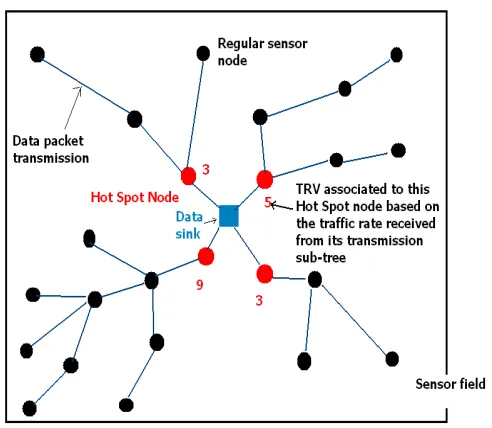
Step 1: The data sink associates a region with each node transmitting to it directly (Hot Spot
node). It assigns the packet rate that it receives from this node as that node’s “Traffic Rate
Value” or TRV. When deciding its motion trajectory, the data sink give priority to those nodes
with high TRV, since the TRV represents the node density of the sub-region transmitting through
the Hot Spot node.
have received data packets from the sensors located at the very extremity of their transmission
sub-tree. Those data packets need to be forwarded from lower to upper node towards the Hot
Spot node, and finally to the sink. Thus, it takes a time period for all Hot Spot nodes to transmit
at their full traffic rate capacity. If the sink needs to assign TRV based on those traffic rates it has
to wait a certain time before doing so. This is called Observation Period (T_obs).
In a network where all nodes transmit data packets periodically as the one we are studying,
the determination of T_obs becomes trivial: the data sink must keep track of traffic rates received
from each 1-hop away node. Then, it considers T_obs as over when all those nodes transmit at a
regular rate for consecutive instances. To avoid any discrepancy due to the noise/packet collision
in the field, the data sink can impose a threshold to reach for consecutive transmission rates per
Hot Spot node before considering T-obs over.
Once T_obs passed, the data sink assigns TRV to all Hot Spot nodes based on the last traffic
rate recorded.
In our model, we set the TRV of a Hot Spot node to the traffic rate that it transmits to the data
sink. (Note that other criteria are also possible, such as residual energy, a combination of traffic
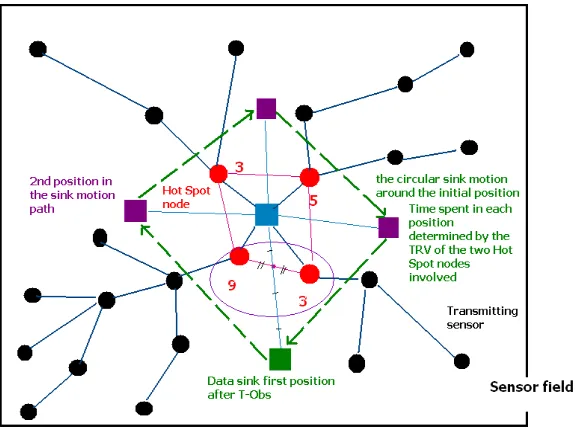
Figure 3: TRV assignment for Hot Spot nodes after time T_obs
Step 2: After the Observation Period, the data sink must assess the succession of positions
that it will evolve to, based on the TRV of each Hot Spot node. Three concerns are raised:
•What is the first position it should move to?
•What order/direction should it take?
•How does it determine the exact spatial position it should move to at each
displacement on the path?
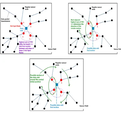
First position: the sink, could pick the Hot Spot node with the highest TRV and move to a
certain extent within that node’s transmission sub-tree. Instead, the sink rather moves in a
location between the two sub-trees of the two nodes with the highest sum of TRV. This motion
forces a more efficient system tree restructuring relieving two Hot Spot nodes instead of one in
one motion. More displacement patterns are applicable (see Chapter VI). If there is more than
Position ordering: once the first position is determined (exact spatial location will be detailed
in the next paragraph), the sink must evolve around the network in an organized fashion, feasible
in a real-world application. The sink must not be expected to jump from one extremity of the
network to the other. That is why ordering the successive positions of the path can not be
achieved by a descending ordering of TRV.
We opted for a circular motion around the network’s center since it is the position where the
sink is placed generally when initially disposing the nodes in the field [7].
The second position on the path is determined by the highest sum of TRV of the Hot Spot
nodes that are already involved in the first position determination. Following the same pattern,
the sink places the rest of the nodes in a geographical, circular order and moves periodically
between two consecutive sub-trees, producing a smooth circular motion around the center.
The only knowledge the sink has of the geographical topology of the sub-trees can be induced
from the spatial location of their respective roots: the Hot Spot nodes. Using the directional
reception antenna, the sink has the ability to list the Hot Spot nodes in a circular order after
determining the first position as the starting point and the second position assessing the rotation
Figure 4: Determination of the sink's circular motion around the initial center position.
Note: In most wireless sensor networks the sink is initially placed in an approximate central
position within the sensor field. The initial position of the sink in our mobile scheme will be set
to the center of the network for the duration of the Observation period. That allows the sink to
have a better assessment of the network traffic pattern [9] before doing its first motion. The
central position is also the sink’s optimal position when it is fixed over a large dense sensor
OSP =(∑(P(x)*T(x))/∑(T))
Where the summation is for all nodes in the network, P(x) represents the location of node x,
and T(x) represents the traffic generation of node x.
Exact spatial sink positioning: The exact positioning of the sink between two regions is
important: the length of the sink’s displacement in that area will determine the extent of the
transmission tree reconstruction. If the distance is insignificant, the Hot Spot node problem is
only pushed to the next sub-node(s) in the tree. If great enough, the transmission topology
changes (see Figure 2).
The exact position between two regions is determined as follows:
a/ We find the center position C(xc,yc) between the two Hot Spot nodes n1(x1,y1), n2(x2,y2)
that are roots of the two concerned sub-trees.
b/ We draw a line from the initial data sink position to that center position C. The distance
between the initial sink position Co(xo,yo) and C is D.
c/ On the same direction of the line drawn we shall place the sink’s new position on a distance
(2*D) from the center of the two Hot Spot nodes in position New(X,Y).
xc = (x1 + x2) / 2 , yc = (y1 + y2) / 2
X = (3 * xc) – (2 * xo)
Y = (3 * yc) – (2 * yo)
‘New’ will be one of the positions of the sink in its motion path when relieving these two
Figure 5: determination of the exact position of the mobile sink between two sub-trees
The sink has no means in figuring out the exact layout of the sub-trees within the sensor field.
Nevertheless, for a high density network (over 5 sensors/meter square) this algorithm seems to
determine an acceptable positioning of the sink at an approximate equal distance from the two
sub-trees involved and provides efficient restructuring of the traffic pattern in that area as it will
be illustrated in our performance evaluation (Chapter IV).
Step 3: The displacement of the data sink between system transmission sub-trees must
provide fairness in balancing the energy consumption among them. When assessing a position
between two sub-trees it also needs to assess a time span for that position. It assesses the time
that needs to be spent in each position based on the traffic rate that it receives from each Hot
Spot node. Therefore, the time span is relative to the TRV associated to those two sub-trees root.
The sink moves in-between the two sub-trees (R1, R2) and stay in that position for a time
T (R1,R2) = k * (TRV(R1) + TRV(R2))
Where T(R1,R2) is the time spent between region1 (R1) and region2 (R2), TRV (R1) is the
TRV associated with the Hot Spot node that is the root of the sub-tree R1 and k is the loitering
constant set to 0.01 in this work.
For each in-between region the sink estimates the time to spend still in that area based on this
formula.
In these three steps, (1) the sink has established a traffic pattern for the network and assigned
a value for each Hot Spot node representing the traffic volume that it receives from its sub-tree;
(2) the sink has assessed ordered positions between each pair of those sub-trees; (3) the sink has
assessed the time spans for each position based on the sub-trees traffic rate.
Figure 6 illustrates the determination of the sink’s motion path in the mobile data sink scheme
based on the Hot Spot nodes’ TRV and their geographical locations in the sensor field:
III.3 Cost & Overhead:
Our main concern with this new technique is the computation cost for restructuring the
transmission tree and adapting the forwarding of the information according to the spatial
evolution of the sink.
Many schemes that consider sink mobility, including SEAD [6], force the mobile data sink to
always communicate with an “access sensor” or “gate”: the sink knows the its gate’s spatial
position, transmits its changing position and gets all data packets from the sensor field through
that gate. This gives us a better understanding of why sink mobility in those schemes is not
meant to decrease the Hot Spot effect, since the gates are Hot Spot nodes.
Our approach is based on an important fact: the data sink is equipped with much greater
energy resources and transmission capacity than the rest of the network sensors. Therefore, our
scheme takes full advantage of that inequality: it relies heavily on the sink ability to inform the
sensors about every displacement and help them assess the most appropriate neighbor to transmit
to.
Second important fact: packet reception cost is several orders less energy-costly than a packet
transmission. In our scheme, the sink broadcasts its new position and by doing so the node can
always determine to which neighbor node it shall transmit just as if the data sink was in fixed
position. The sensor having spatial information about all its 1-hop away neighbors, the
directional transmission is computable by a majority of sensor models.
We argue that such a technique does not increase the transmission overhead. This is mainly
because such broadcast takes place in a fixed sink network as well: the sensors being by design
the data sink is mobile or not. Transmitting nodes need to adapt constantly to the collapse of their
neighbors when forwarding their information towards the sink.
For example, our scheme may then be combined to the one proposed by Li and Halpern [5] so
that each node always determines the minimum energy path towards the sink once it
acknowledges its position. This approach is based on “echo packets” that the data sink sends
towards the data sink through all possible paths and the cost of each path is recorded as the
packet is forwarded from lower to upper node in the tree. The sink eventually receives the packet
and sends a packet back informing the transmitting node of the optimal path. The process needs
to be redone periodically because of all the sensors that collapsed between two “echoes”. In our
case, the time span could be set to the time-spans spent in each new sink position within its
motion path .We leave this as our future work.
Note that our scheme does not require the knowledge of an energy map for all nodes as it has
been proposed in the past [11]: a transmitting node always transmit to the same 1-hop away
neighbor towards the sink until that nodes die. Then, it finds the next best placed neighbor to
transmit to. The transmitting nodes within the network are not responsible for balancing the
energy consumption among neighbors. The sink in motion is the only factor in balancing the
energy usage.
Maintaining an energy map is very costly because it requires many transmissions/receptions
between neighbor nodes to keep the maps accurate. It can become a significant negative factor
whenever the network density is increased.
In our technique, nodes in their transmitted packets won’t have to forward information about
transmission but becomes significant when considering the totality of transmissions over a
network lifetime.
The extra computation cost at the data sink is limited. Note that this is also related to the
Loitering Constant.
The only energy that needs to be considered as additional for a mobile scheme is the one that
the data sink itself uses to move around the network but as assumed above it can be considered
as a larger device with “unlimited energy resources”; the nodes will also use extra energy
receiving “location packets” from the sink (for every new position it takes) and will use energy
computing those information, but both of those costs can be neglected compared to the one of
IV Performance Evaluation:
IV.1 Methodology:
Before we can implement our mobile data sink scheme, we need to create an accurate
wireless sensor network model to be able to compare throughputs. The model needs to be as
close to real life applications as possible. We must be able to determine the optimal sink position
for any network topology and also determine a thorough multi-hop packet transmission among
nodes.
An energy consumption model is needed to determine the energy ratio deducted from the
node’s reserves after each transmission (E {trans}).
The energy consumption model for a packet transmission is the following:
E_{trans} = D^w + k
where D is the distance between the source and the immediate receiver, k is the constant
energy consumption (set to 10 in this work), unrelated to distance, and w is the path loss
exponent (assumed to be 2 in this work)
If node P transmits N number of data packets to node Q, the energy consumption for packet
transmissions from the power resources of node P are N * E {trans}.
Energy consumption for packet reception being several orders of magnitude smaller than the
one for a packet transmission [8], it will not be taken into consideration in this work.
IV.2 1D network:
We investigate a 1-dimensional network of 1000 meters containing N=100 nodes, which are
distributed on a line. All nodes have the same initial battery level, 10^5, except the data sink that
has unlimited resources. The transmission range of each sensor is set to 20 meters. In the
transmissions, we choose a multi-hop transmission where each node transmits to the closest node
“alive” towards the sink.
The data sink is moved along that network. For each position, we estimate the network
lifetime considering heterogeneous traffic pattern in the network: high node density regions and
high traffic rate regions.
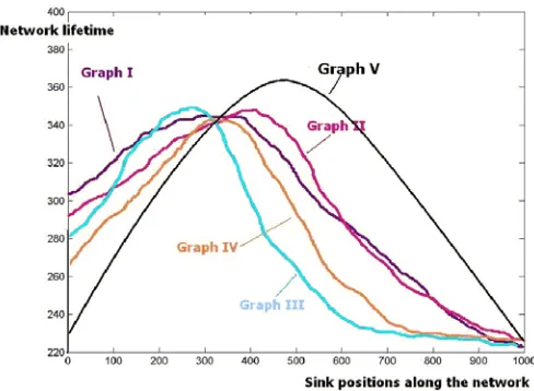
Figure 7 provides an illustration of the optimal sink position determination considering those
features in a 1-D network. The network lifetime as a function of the data sink's location is shown.
Graph I represents the network lifetimes according to the sink position when 30% of the nodes
are located within the area [200,300] of the network (the rest of the nodes are placed in the other
regions randomly). Graph II represents the network lifetimes according to the sink position when
all nodes within the area [200,300] have twice the transmission rate of the rest of the nodes of the
network (all nodes in that case are evenly spread along the linear network). Graph III is similar to
Graph I but 50% of the nodes are within [200,300]. Graph IV is similar to Graph II but the nodes
in [200,300] transmit 4 times the number of packets the nodes in other regions of the network do.
Graph V finally represents the base case: nodes evenly distributed along the network with equal
Figure 7: Impact of high traffic rate and high node density regions on the optimal data sink position within 1D network
Obviously, the optimal data sink in both cases shifted from its central position (Graph V)
towards the high traffic rate region (338 for Graph I, 442 for Graph II, 282 for Graph III, 347 for
Graph IV).
Interestingly, the optimal sink location “reacts” similarly to high traffic rate regions and high
node density regions since a node transmitting twice more packets than another node could be
thought of as two nodes in the same location transmitting the same number of packets as all other
nodes.
After comparing the values of the network lifetime for a large set of traffic patterns,
alternating equivalent increment in traffic rates and node density within the same regions (as
illustrated in Figure 7), the following induction could be stated: we consider heterogeneity of
IV.3 2D network - Assumptions: Our 2-D network model is designed as follows:
•Network is a 100x100 array containing 100 nodes: 1 node per meter square (our
network node density is conform to usual wireless sensor network high node densities as
seen in [7,8]).
•The network is considered “dead” when 40% of the nodes have exhausted their
batteries. This percentage is acceptable [7] since most researches consider that a network
is in the “high collapse risk level” when more than a third of its sensors have exhausted
their power resources.
•All nodes have similar transmission rates and a 10^5 energy unit initial battery level,
the energy consumption for each packet transmission being the one proposed above (E
{trans}).
•All nodes use a hybrid energy map: instead of keeping track of the energy level of
each 1-hop way sensor and dispensing energy resources maintaining that energy map, the
transmitter only keeps track of the ability of its neighbors to retransmit a single packet.
This relies on the action on the receiver side: when a sensor transmits packets from a
lower to an upper node in the tree structure, it informs the lower node when reaching a
“danger state”. When that state is reached, the “router node” will not have the necessary
energy resources to retransmit packets in the future and will probably send an extra
information packet of its own before collapsing. The lower node being informed of that
will not lose energy transmitting towards that node and transmits instead to the next
Thus, multiple unnecessary transmissions to a “dead node” are avoided and a level of
energy awareness among 1-hop away nodes is instated without excessive
energy-informative data sent back and forth.
•Multi-hop packet transmission: each node has a 20 length unit transmission range and
transmits its packets to the closest node within that range that is closer to the sink, if that
node is still “alive”. The neighbor node must be 1-hop away from the transmitter on an
established path towards the sink. Initial path establishment from node to sink will not be
detailed in this work since it is based on the same approach as any basic wireless sensor
network.
If no such neighbor node exists, the transmitter keeps increasing its range until it can
reach, but will exhaust more energy doing that [7] since its energy consumption per
transmission is proportional to the distance to the receiving node/sink.
Notes:
•The Hot Spot node never being farther than 20 length units from the sink’s initial
position (because of restraints on their transmission range) mathematically the data sink
in determining its motion path will never surpass the network limits. In fact, it hardly
ever exceeds the 60 length unit displacement. In WSN, the transmission range hardly
exceeds a tenth of the network’s radius. Our scheme implies then that the sink
displacement never exceeds a third of the network’s radius, which reflects the “real life”
realism of the scheme that we are proposing: not expecting from the data sink to reach the
•In this work, we neglect the time for the mobile data sink moves from one location to
another location. While such movement isn't instantaneous, we argue that the data
transmission periods are usually higher than the time needed to complete the movement.
IV.4 Results:
All our simulations have been run on Matlab 6.5, and our data set consists of 100 different
network topologies generated by our program.
IV.4.1 Mobile vs. Fixed Data Sink:
The energy transmission analytical formula helped determine the optimal sink position in a
2-D network relying on the knowledge of the geographical location of the nodes and their traffic
rates. We estimated the average lifetime of the network over the data set using each network’s
optimal, fixed sinkposition. The average lifetime was equal to 140.65 time units.
Afterwards, we ran the same number of tests over the same set applying the mobile sink
algorithm and the average network lifetime was equal to 187.75 time units. The lifetime
extension is equal to 33.48%.
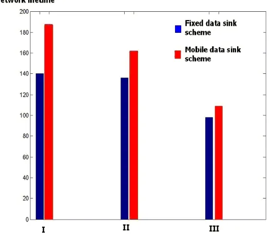
Figure 8 presents the comparative throughputs for fixed and mobile data sink schemes. Plot I
represents the network lifetime considering our 2D network model; plot II represents the network
lifetime when the number of nodes is multiplied by 1.5 (150 nodes); plot III represents the
network lifetime when the node traffic rate is doubled.
The results clearly show that the mobile data sink approach outperforms a network with a
explained as follows: when the node density is too large, there are many nodes suffering the hot
spot effect and it is difficult for the mobile data sink to cover all such nodes.
Figure 8: Comparative network lifetimes for fixed sink network and network implementing the Mobile Data Sink scheme with variable node density and data traffic rate
Our second goal was to have a better distribution of the energy consumption among the
network nodes.
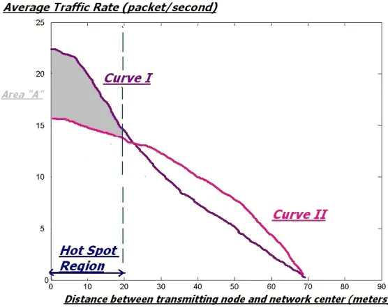
Figure 9 displays the standard variance of the traffic rates of all nodes within distance d of the
network center. The variance is estimated over the average transmission rate per node over each
node’s lifetime. The results were measured prior to any node dies.
Curve I represents the standard variance of the transmission traffic rates among nodes when
Figure 9: Comparative standard variance of traffic rate among nodes for both fixed and mobile data sink schemes.
Over a hundred different network topologies, the average global traffic rate within the Hot
Spot region nodes for a fixed sink scheme was 171 packet/second, while the average for a mobile
data sink scheme was 121 packets/second. The traffic rate decrease within the Hot Spot area is
equal to 41.32%. That difference is represented by area A in Figure 9.
Meanwhile, the traffic rate among the rest of the nodes, excluding the leaves of the
transmission tree, is greater by 41.32% when using the mobile sink scheme, but that traffic
increase is distributed among a larger number of nodes. In fact, the average traffic rate for
regular nodes is 8.3 packet/second for a mobile sink scheme while it equals 5.2 packet/second for
a fixed scheme. This explicitly demonstrates the better distribution of energy consumption
among the network nodes and the reduction of the Hot Spot effect on the network.
the data sink position at the moment of their “death”. Note that these curves only represent the
40% of nodes that died causing the network collapse.
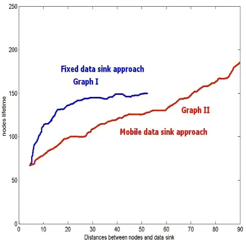
Figure 10: Comparative average distribution of energy consumption among network nodes for fixed and mobile data sink schemes.
By comparing the two curves, we see clearly that graph II representing the mobile data sink
approach extends further and has a smoother slope than graph I, representing the fixed data sink
approach. Three points can be made in that matter:
First, the maximum value of graph II (approx. 180 time units) is greater than the one for graph
I (approx. 142 time units), and that tells us explicitly that the network has a longer lifetime
using a mobile data sink: the last node to die (after what the network collapses) has a greater
lifetime value for Graph II, and that node’s lifetime is equal to the network lifetime since after its
Second, the slope of graph I (fixed sink) is greater than graph II, which can be explained by
the fact that the closest nodes to the sink in a fixed sink approach die very quickly while the ones
just a little further die considerably slower (which reflects a bad distribution of the energy
consumption in that area); while the slope for a mobile data sink is smaller which tells us that the
nodes that are very close to the sink die almost at the same time as the ones much farther from it,
and that is what we wanted in a matter of normalized distribution of the energy consumption
over the network nodes.
Third, graph II spreads larger than graph I, which finally tells us that some of the nodes that
are much farther from the data sink have also exhausted their energy resources while the
shortness of graph I tells us that most of the nodes involved in the “heavy” packet transmissions
(fastest to die) are the ones closest to the data sink (direct illustration of the Hot Spot effect). We
can get from that a second proof of the normalization of the energy consumption among nodes
and the fact that more nodes within the network are involved in the retransmissions when
applying a mobile data sink approach.
IV.4.2 Mobile Data Sink scheme vs. Energy Balanced Propagation scheme [4]:
We propose to compare throughputs between our Mobile scheme and the Energy Balanced
Propagation scheme [4]. The test will be run on a set of 100 different network topologies.
The Energy Balanced Propagation scheme serves the same purpose as our work: normalize
the power consumption among all nodes to extend the network lifetime. It is based on a
probabilistic approach determining if a sensor node should transmit to a neighbor sensor towards
forwarding. The transmission decisions over a node lifetime help reduce the packet forwarding
among neighbor sensors and decrease consequently the Hot Spot effect, based on the heavy
forwarding towards the sink.
We compared our scheme to [4] and Figure 11 displays the comparative results:
Figure 11: Comparative throughputs in standard variance of node traffic rate and network lifetime for Mobile sink and Energy Balanced Propagation schemes.
The first figure (left) compares standard variance of node traffic rate against distance between
transmitting node and sink for the two schemes. Curve I stands for the Mobile Data sink scheme
while Curve II represents the standard variance for the Energy Balanced Propagation scheme.
When comparing the slope of the curves we can induce that the Energy Balanced Propagation
algorithm leads to a more efficient normalization of the traffic rate, and therefore a more efficient
normalization of the energy consumption among the network sensors than the Mobile Data Sink
scheme.
It also reduces more efficiently the Hot Spot effect within the network since the average
scheme by -2.3 packets/second (11.3 packets/second for balanced scheme vs. 13.6
packets/second for mobile sink scheme).
On the other hand, when comparing average network lifetimes for the two approaches we can
notice on the second figure (right) that the Mobile Data Sink is more efficient than the balanced
scheme.
Result (I) is obtained from simulations on our 2D model. Result (II) is obtained when
increasing the number of sensors by 1.5. Result (III) is obtained when doubling the node traffic
rate.
In all scenarios our scheme leads to a longer network lifetime and outperforms the balanced
approach respectively by 5%, 13% and 36%.
The important gap in lifetime extension when increasing the traffic rate for the sensors can be
explained by the fact that nodes in the balanced scheme exhaust an important amount of energy
when they decide to transmit directly to the data sink instead of a neighbor sensor. The energy
transmission cost being related to the distance between transmitter and receiver (see IV.1), the
high number of packets to transmit at a high cost reduces severely the average node lifetime and
therefore the network lifetime as well.
We can now make the following observation: normalizing the traffic rate among nodes
implies extending the network lifetime only if the average energy consumption per transmission
is kept equal or smaller than its initial value.
In this comparative case, the balanced scheme leads to a more balanced traffic pattern among
sensors and a more efficient reduction of Hot Spot effect, but their average energy consumption
Note: The probability pattern used when making the transmission decision for the Energy
Balanced Propagation scheme has been simplified from its original version but does not affect
the scheme throughput in any ways. Comparative results to our basic fixed sink network’s
throughput confirm it.
IV.4.3 Mobile Sink scheme using Hybrid Energy Map vs. Fixed Sink scheme using Node
Energy Map [11]:
In research [11] is detailed the use of an energy map scheme. According to the scheme, all
nodes use a list of energy level of their 1-hop away neighbor sensors and maintain that energy
map through several energy-related communications. Whenever a node needs to transmit a data
packet it consults its energy map to decide which the appropriate neighbor to transmit to is. It
balances the number of packets it sends to all neighbors so that the forwarding load is shared
when packets are going from the bottom to top of the transmission tree.
Our scheme uses a variant of the Energy Map scheme that we call Hybrid Energy Map: the
transmitter only keeps track of the ability of its neighbors to retransmit a single packet (see IV.3
for details).
The variation proposed in our scheme aims to reduce the unnecessary energy consumption
when sending a high number of informative packets about power levels among neighbor nodes.
Our scheme affords not using a regular energy map because the normalization of energy
consumption among network sensors is based on the sink motion and not on the Energy Map
scheme. The Hybrid model allows the transmitting node the minimum necessary information
To prove the sufficiency of our Hybrid energy map for the Mobile Sink algorithm and its
superiority to a regular wireless sensor network using an Energy Map algorithm we compare
throughputs of both implementations over a set of 100 different network topologies.
Figure 12: Comparative throughputs in network lifetime and standard variance of node traffic rate for Mobile sink scheme and fixed data sink using the Energy Map scheme.
From the figure on the left we notice that the Mobile scheme offers longer lifetime to the
network than a network with a fixed sink using the map. For our 2D model (I) it outperforms the
map scheme by 4%; for the 2D network with 150 sensors (II) it outperforms significantly the
map scheme by 17%; for the 2D model with a doubled initial node traffic rate (III) it outperforms
the map scheme by 4% as well.
The difference of efficiency between the two schemes is high for high node density networks
because it implies more proximity among sensors, which leads to a high ratio of neighborhood
among nodes. Therefore it requires a high traffic rate among those neighbors just to maintain the
energy maps and the power consumption for those transmissions reduces consequently the
On the other hand, the Hybrid approach does not imply an important increase in the “energy
map maintenance traffic” since the ratio of transmission per new node in the region is equal to an
extra informative transmission to the lower nodes in the tree when that node can not forward
their packets anymore.
The energy saving using the Hybrid scheme becomes crucial whenever the network node
density is increased and the network is already using a scheme to balance the energy
consumption among the sensors.
From the second figure (right) we can finally conclude that using the energy map does not
efficiently reduce the Hot Spot effect in the network in comparison to our Mobile data sink
scheme. The average traffic rate in the Hot Spot region is 156 packets/second for the Energy
Map scheme while equal to 121 packets/second for our Mobile Sink scheme.
The Map usage helps balance the packet distribution among neighbors, but in a tree structure
the number of neighbors decreases gradually when narrowing towards the root and ultimately all
packets will still be transmitted through the Hot Spot nodes. The slight decrease in the Hot Spot
effect is then due to the possibility of sensors having more than one Hot spot node within their
V Conclusion:
We have proposed a mobile data sink technique to extend the network lifetime.
The mobile data sink is designed to move towards the high node density and traffic regions
and to relieve the nodes that are responsible for forwarding the information from those regions to
the sink. The determination of the sink’s timed motion path has been detailed thoroughly and the
purpose of each displacement feature has been given. The round-robin motion among the
overloaded traffic regions of the network balances the power consumption among the network
sensors and ultimately extends the network lifetime.
Throughout extensive simulations, we have shown that our scheme extends the network
lifetime by more than a third, compared to a fixed data sink approach. We have also proposed
comparative throughputs with networks using an Energy Balanced Propagation scheme and
networks using an Energy Map.
The performance gain has been shown to be achieved through balancing the traffic rates of all
nodes in the hot spot region without increasing the average energy consumption per
transmission. Also, using a Hybrid Energy Map that allows a transmitting node partial
knowledge of the energy pattern surrounding it proved to be sufficient to outperform a basic
network with a fixed data sink using an energy map.
Finally, the efficiency of our scheme in comparison to the two mentioned above has been
proven when altering the network node density and the sensors’ initial traffic rate and produced
VI Future Work
Through our model we tried to come as close as possible to a real-world situation.
Nevertheless, the breadth in wireless sensor network topologies and traffic patterns leaves room
for many possible improvements to our scheme.
The multitude of parameters that need to be considered when implementing the Mobile Data
Sink scheme allow further research to optimize the path determination during the motion.
For instance, when the data sink is in the idle time determining the positions it must take and
the time period it must spend in each of these positions, it will not adapt to the network evolving
topology once it leaves that initial central position. Although the constant transmission tree
restructuring might change the traffic pattern after the first motions of the sink.
One could explore how much the network lifetime can be extended if the data sink could
adapt at each step: decide to reduce the time spent within a high density region or even skip that
position because a farther region might have a higher priority within the updated pattern.
More parameter values can be shifted in order to reach a longer network lifetime:
•the exact spatial positioning of the sink during the motion can be modified to allow
the sink to go farther (or not) inside the Hot Spot regions;
•The time span in each region can be proportional to the residual energy resources of
the neighbor nodes. If our scheme is combined to an Energy Map (non Hybrid) scheme,
the time slot determination might be more efficient.
It would be also interesting to evaluate the trade-off of the scheme for an entire mobile
network where mobility is considered for regular nodes as well, as it might be the case in
wireless sensor networks. May be in that case our technique could be introduced in a multi-sink
Other combined schemes can be considered: using an Energy Map in our Mobile Data Sink so
that the energy consumption normalization is factor of the sink mobility and the sensors’ local
power knowledge.
Finally, the throughput of the scheme could be tested on a network with multiple data sinks
Reference
s
[1]J.-H. Chang and L. Tassiulas, “Routing for maximum system lifetime in wireless ad-hoc
networks,” in Proceedings of 37-th Annual Allerton Conference on Communication, Control,
and Computing, Monticello, IL, Sept. 1999.
[2] Stefano Chessa1 and Paolo Santi2, ”Crash Faults Identification in Wireless Sensor
Networks”, Dipartimento di Informatica, Univ. of Pisa, Italy; Istituto di Matematica
Computazionale del CNR, Pisa, Italy, 2002.
[3] Konstantinos Kalpakis, Koustuv Dasgupta, and Parag Namjoshi “Efficient Algorithms for
Maximum Lifetime Data Gathering and Aggregation in Wireless Sensor Networks1;2”
[4] Charilaos Efthymiou Computer Technology Institute University of Patras, Sotiris
Nikoletseas; Computer Technology Institute University of Patras, Jose Rolim University of
Geneva, “Energy Balanced Data Propagation inWireless Sensor Networks”, 2002.
[5] Li Li Joseph Y. Halpern, Dept. of Computer Science Cornell University,
“Minimum-Energy Mobile Wireless Networks Revisited”
[6] Hyung Seok Kim School of Electrical Engineering. Seoul National University, Tarek F.
of Electrical Engineering, Seoul National University, “Minimum Energy Asynchronous
Dissemination to Mobile Sinks in Wireless Sensor Networks”
[7] I.F. Akyildiz, W. Su, Y. Sankarasubramaniam, E. Cayirci, Broadband and Wireless
Networking Laboratory, School of Electrical and Computer Engineering, Georgia Institute of
Technology, “Wireless sensor networks: a survey”
[8] Ian F. Akyildiz, Weilian Su, Yogesh Sankarasubramaniam, and Erdal Cayirci, Georgia
Institute of Technology, “A survey on sensor networks”, 2002
[9] Katayoun Sohrabi, Jay Gao, Vishal Ailawadhi and Gregory J Pottie, Electrical
Engineering Department UCLA, “Protocols for Self-Organization of a Wireless Sensor
Network”, 2002
[10] Jae-Hwan Chang and Leandros Tassiulas, Department of Electrical and Computer
Engineering & Institute for Systems Research, University of Maryland at College Park, “Energy
Conserving Routing in Wireless Ad-hoc Networks”
[11] Raquel A. F. Mini , Badri Nath , Antonio A. F. Loureiro, Department of Computer
Science Federal University of Minas Gerais, Department of Computer Science – Rutgers
University, “Prediction-based Approaches to Construct the Energy Map for Wireless Sensor
Vita
Yacine Chikhi was born in Algiers, Algeria in 1982. He grew up in Algeria and studied in Arabic
until passing his Baccalaureat (High school final test) in June 1999. He then moved to live in
Paris, France and got admitted in the DEUG MIAS program at Pierre & Marie Curie University.
He earned his “Licence d’Informatique” (3rd year diploma in computer science) and was
accepted in an international exchange program with the University of New Orleans to complete
his bachelor degree. After graduating from his French university, Yacine was accepted in the
Master program in Computer Science of UNO in January 2004. He defended his thesis in April
2006 and decided to apply for the Master program of the National Superior School of