Volume 32 - Article 24 | Pages 723–774

(1)

DEMOGRAPHIC RESEARCH

VOLUME 32, ARTICLE 24, PAGES 723

−

774 PUBLISHED 13 MARCH 2015

http://www.demographic-research.org/Volumes/Vol32/24/ DOI: 10.4054/DemRes.2015.32.24

Research Article

Quality of demographic data in GGS Wave 1

Jorik Vergauwen

Jonas Wood

David De Wachter

Karel Neels

This publication is part of the Special Collection on “Data Quality Issues in the First Wave of the Generations and Gender Survey,” organized by Guest Editors Aart C. Liefbroer and Joop Hox.

©2015 Vergauwen, Wood, De Wachter & Neels .

This open-access work is published under the terms of the Creative Commons Attribution NonCommercial License 2.0 Germany, which permits use, reproduction & distribution in any medium for non-commercial purposes, provided the original author(s) and source are given credit.

(2)

1 Introduction 724

2 Theoretical framework: the total survey error approach 726 2.1 Issues related to selecting respondents 727

2.1.1 Sampling error 727

2.1.2 Coverage error 727

2.1.3 Nonresponse at the unit level 728 2.2 Issues related to response accuracy 730

2.2.1 Item nonresponse error 730

2.2.2 Measurement error due to the respondent 732 2.2.3 Measurement error due to the interviewer 733

2.3 Survey administration issues 734

2.3.1 Mode effects 734

2.3.2 Post-survey error 734

2.3.3 Comparability effects 734

2.4 Assessing total survey error 735

3 Data & methods 736

3.1 Harmonized data files 737

3.2 Retrospective estimation of age-specific rates 739 3.3 Period total female first-marriage rate and period total fertility rate 741 3.4 Period mean age at female first marriage and period mean age at

childbearing

741

3.5 Cohort total female first-marriage rate and cohort total fertility rate 742 3.6 Cohort mean age at female first marriage and cohort mean age at

childbearing

742

3.7 Indicators of survey error 743

4 Results 743

4.1 Cohort total female first marriage rate and mean age at female first marriage

744

4.2 Period total female first-marriage rate and mean age at female first marriage

748

4.3 Cohort total fertility rate and mean age at childbearing 753 4.4 Period total fertility rate and mean age at childbearing 758

5 Discussion and conclusion 762

5.1 Main findings 762

5.2 Potential sources of survey error in GGSWave 1 763 5.3 Challenges for future research 765

6 Acknowledgements 765

(3)

Quality of demographic data in GGS Wave 1

Jorik Vergauwen1

Jonas Wood2

David De Wachter3

Karel Neels4

Abstract

BACKGROUND

A key feature of the Generations & Gender Programme (GGP) is that longitudinal micro-data from the Generations and Gender Surveys (GGS) can be combined with indicators from the Contextual Database (CDB) that provide information on the macro-level context in which people live. This allows researchers to consider the impact of socio-cultural, economic, and policy contexts on changing demographic behaviour since the 1970s. The validity of longitudinal analyses combining individual-level and contextual data depends, however, on whether the micro-data give a correct account of demographic trends after 1970.

OBJECTIVE

This article provides information on the quality of retrospective longitudinal data on first marriage and fertility in the first wave of the GGS.

METHODS

Using the union and fertility histories recorded in the GGS, we compare period indicators of women’s nuptiality and fertility behaviour for the period 1970–2005 and cohort indicators of nuptiality and fertility for women born after 1925 to population statistics.

1_{Corresponding author. University of Antwerp, Belgium. E-Mail: [email protected].} 2_{University of Antwerp, Belgium.}

3

University of Antwerp, Belgium.

(4)

RESULTS

Results suggest that, in general, period indicators estimated retrospectively from the GGS are fairly accurate from the 1970s onwards, allowing exceptions for specific indicators in specific countries. Cohort indicators, however, were found to be less accurate for cohorts born before 1945, suggesting caution when using the GGS to study patterns of union and family formation in these older cohorts.

CONCLUSIONS

The assessment of the validity of demographic data in the GGS provides country-specific information on time periods and birth cohorts for which GGS estimates deviate from population statistics. Researchers may use this information to decide on the observation period or cohorts to include in their analysis, or use the results as a starting point for a more detailed analysis of item nonresponse in union and fertility histories, which may further improve the quality of GGS estimates, particularly for these earlier periods and older birth cohorts.

COMMENTS

Detailed country-specific results are included in an appendix to this paper, available for download from the additional material section.

1. Introduction

In 2000 the Population Activity Unit (PAU) of the United Nations Economic Commission for Europe (UNECE) launched the Generations and Gender Programme (GGP) to enhance understanding of the causes and consequences of demographic change in developed countries (Vikat et al. 2007). International comparability is a key feature of the GGP and several, mainly European, countries have become highly committed to the implementation of the programme. The GGP consists of two pillars. The first pillar is a set of Generations and Gender Surveys (GGS)5. The GGS is a panel survey that collects longitudinal micro-level data on a representative sample of non-institutionalized residents aged 18 to 79 years in each of the participating countries. The first wave of the GGS collects detailed data on partnership histories and (non-)resident children, making it possible to reconstruct changes in union formation and fertility in recent decades and link these to covariates at the individual, household, and contextual levels. To overcome the limitations associated with the retrospective design of the Fertility and Family Surveys (FFS) – the immediate predecessor of the GGP – the GGS

(5)

combines elements of a retrospective setup with a prospective panel design (Vikat et al. 2007). The prospective design makes it possible to assess the impact of characteristics recorded in each wave (e.g., values and intentions) on subsequent behaviours, thus contributing to an enhanced understanding of the dynamic nature of demographic behaviour and the life-course. The Contextual Database (CDB)6 (see the contribution of Caporali et al. in this special volume) is the second main pillar of the GGP and provides aggregate indicators at the meso (regional) and macro (national) levels. The CDB contains 200 indicators organized around 16 domains, covering both quantitative and qualitative information at the aggregate level for each of the participating countries, mostly from the 1970s onwards (Spielauer 2007). The possibility of combining longitudinal micro-level data from the GGS with contextual data from the CDB using multilevel (hazard) models allows for the assessment of the effect of various contexts (e.g., cultural, policy, and economic) on changing demographic and social behaviours (Simard and Franklin 2005; Vikat et al. 2007).

The contextual indicators in the CDB are generally population statistics drawn from different standardized national and international sources (e.g., vital statistics). As a result, the validity of analyses that combine contextual indicators with longitudinal micro-level data critically depends on the quality of the retrospective data on union formation and fertility collected in the GGS. To the extent that partnership and fertility histories provide a biased account of past trends, this may also yield biased estimates of the effect of various contextual factors on demographic behaviour. This also applies to explanatory analyses using GGS micro-data to examine associations between individual-level predictors and partnership and fertility histories. In this paper we use the total survey error approach to discuss potential sources of error in surveys such as the GGS, with a specific focus on bias in retrospectively collected event-histories (Blossfeld and Rohwer 2002; Blossfeld, Golsch, and Rohwer 2007; Weisberg 2009). In line with the GGS sample design guidelines, the paper subsequently aims to assess the joint effect of different sources of error on the validity of demographic data in the GGS by comparing indicators of first marriage and fertility estimated retrospectively from the GGS to population statistics (i.e., time-series drawn from vital registration, census, and register data).

(6)

2. Theoretical framework: the total survey error approach

Retrospective surveys have become the main source of data on partnership and childbearing histories (Beckett et al. 2001; Murphy 2009; Kreyenfeld et al. 2010). We use the total survey error approach to classify sources of error in surveys (Weisberg 2009; Groves and Lyber 2010). In this approach the term ‘error’ refers to the difference between the value obtained from a survey and the true value, usually the true value for the larger population of interest (Weisberg 2009). A characteristic feature of demographic surveys is that the true value for the population (at least for a number of characteristics) is frequently available from population statistics. Although population statistics can be subject to error and have been shown7 to be biased in specific cases (e.g., Velkoff and Miller 1995; Morgan et al. 1999; Aleshina and Redmond 2005), we will consider them as a standard against which the total survey error in the Generations and Gender Surveys can be measured. We consider GGS estimates valid if they reflect the population value without systematic bias (Weisberg 2009).

Differences between population statistics and demographic indicators calculated retrospectively from the GGS may result from different sources of error, which can be classified into three larger types. Section 2.1 discusses the first type of error, which concerns issues related to selecting respondents for a survey. This includes sampling error, coverage error, and error associated with nonresponse at the unit level. Section 2.2 discusses the second type of error, which concerns issues related to response accuracy. This section distinguishes between nonresponse error at the item level, measurement error due to respondents, and measurement error due to interviewers. Finally, section 2.3 discusses the third type of error, which concerns various issues related to survey administration, including post-survey error, mode effects, and comparability effects (Weisberg 2009).

(7)

2.1 Issues related to selecting respondents

2.1.1 Sampling error

Sampling error is the error that occurs when a sample is surveyed rather than the entire population. Systematic bias may result when non-probability sampling is used, whereas probability sampling permits mathematical derivation of the sampling error (Weisberg 2009). Non-probability samples are likely to generate selectivity in the sample to the extent that inclusion probabilities depend on at-home availability patterns of different groups in the population. The random route procedure implemented in the German GGS has, for instance, been shown to induce selectivity (Sauer, Ruckdeschel, and Naderi 2012). However, as most countries implemented probability sampling in line with the GGS sample design guidelines (Simard and Franklin 2005 and Fokkema et al. in this special volume), the next sections focus on the potential impact of coverage error and nonresponse error at the unit level.

2.1.2 Coverage error

Coverage error occurs when the sampling frame does not correspond with the population of interest (Weisberg 2009). A typical issue of coverage error in retrospective surveys such as the GGS is that the collection of event-histories relies on survivors, while these may represent a nonrandom subgroup of their birth cohort with specific characteristics due to selective institutionalization, mortality, or out-migration (Neels 2006; Kreyenfeld et al. 2010)8. Selective institutionalization has been found to affect maternity histories because married women are more likely to have children and less likely to enter a retirement home (Sauer, Ruckdeschel, and Naderi 2012). This may result in an underrepresentation of childless women in non-institutionalized populations at older ages, which in turn can bias fertility levels upward for these cohorts. Similarly, mortality is found to be lower among married and cohabiting individuals than among singles (Gadeyne and Deboosere 2000; Sauer, Ruckdeschel, and Naderi 2012), whereas higher mortality is found for both childless and multiparous women (Kvåle, Heuch, and Nilssen 1994; Gadeyne and Deboosere 2000). This may introduce additional bias in nuptiality and fertility indicators for older cohorts. Finally, immigration and emigration are generally considered to be strongly correlated with patterns of nuptiality and family

8

(8)

formation (Neels 2006; Murphy 2000; 2009; Kreyenfeld et al. 2010; 2011; Sauer, Ruckdeschel, and Naderi 2012). Underrepresentation of migrant groups in surveys is frequently found – e.g., in the German GGS (Kreyenfeld et al. 2010) – and this will lead to an underestimation of nuptiality and fertility when migrant groups have higher marriage or childbearing rates.

2.1.3 Nonresponse at the unit level

Unit nonresponse occurs when a designated respondent does not participate in the survey, thereby limiting how representative the actual respondents are of the population of interest (Weisberg, 2009). Since nonresponse is found to vary significantly between social groups, under or overrepresentation of specific groups may affect the validity of retrospective estimates to the extent that these characteristics are correlated with nuptiality and fertility patterns. Determinants of unit nonresponse frequently discussed in the literature are age, gender, socio-economic position, geographical region, ethnicity, household (com)position, and parity. Unfortunately, the information available in the sampling frame (e.g., registers) is generally too limited to restore the representativeness of the sample with respect to such characteristics via stratification (see Fokkema et al. in this special volume on the calculation of post-stratification weights).

Considering age, younger people are repeatedly found to have lower participation rates in surveys (Van Loon et al. 2003; Neels 2006), whereas other sources mention lower participation rates for both the oldest and youngest age groups (Groves and Couper 1998; Goldberg et al. 2001; Nicoletti and Peracchi 2005). Similarly, Régnier-Loilier (2011), studying attrition between waves 1–2 and waves 2–3 of the French GGS, finds higher attrition for people younger than 30 and for people aged 60 and older. With respect to gender, lower response rates are generally found for men (Van Loon et al. 2003; Nicoletti and Peracchi 2005). Also in the French GGS, higher attrition has been found for men, especially among respondents younger than 50 (Régnier-Loilier 2011).

(9)

Winter 2011), or income characteristics (Bergstrand et al. 1983; Fitzgerald, Gottschalk, and Moffitt 1998) mostly find higher response rates for higher socio-economic groups. Also in the case of the German GGS, differential response rates by socio-economic position have been found to lead to an overrepresentation of higher social strata (Kreyenfeld et al. 2010). For the French GGS, Régnier-Loilier (2011) suggests that attrition is highest among lower-educated individuals and unemployed persons. Similarly, Burkimsher (2009) states that the underestimation of fertility for older cohorts in the Bulgarian, Hungarian, and Georgian GGS may be due to the underrepresentation of older women with low SES, since lower education in these cohorts is correlated with having more children.

Geographical region plays an important role, as response rates are often found to vary strongly between regions (Goldberg et al. 2001; Neels 2006), with response rates generally being particularly low in urban regions (Groves and Couper 1998; Abraham, Maitland, and Bianchi 2006). For the French GGS, Régnier-Loilier (2011) has found that attrition is highest in urban regions. For the GGS in Central and Eastern European countries it has been suggested that rural residence may be correlated with both higher fertility and lower participation rates and thus may provide a partial explanation of underestimation of fertility (Burkimsher 2009).

Ethnicity is another characteristic related to lower response rates that may induce bias in nuptiality and fertility indicators. Migrant populations are generally underrepresented in surveys, particularly when the availability of the questionnaire in different languages is limited (Festy and Prioux 2002; Kreyenfeld et al. 2010). Foreigners are frequently found to show higher degrees of unit nonresponse (Bergstrand et al. 1983; Neels 2006), resulting in an underrepresentation of these groups (see Kreyenfeld and colleagues (2010) with respect to the German GGS). Several contributions have discussed the confounding role of migration (e.g., the role of East-West migration in Germany in higher fertility (Kreyenfeld et al. 2010)) or ethnic minorities in the GGS (e.g., underrepresentation of Roma populations with considerably higher fertility in Central and Eastern Europe (Burkimsher 2009)). Also, results for the French GGS (Régnier-Loilier 2011) indicate that attrition is higher for migrant groups.

(10)

context of a household-based sample, Groves and Couper (1998) find a strong negative correlation between the number of household members and the number of contact attempts required to reach designated individuals in households.

Finally, higher parityhas been shown to be associated with higher participation in surveys (Nicoletti and Peracchi 2005; Neels 2006), whereas unit nonresponse is higher in single child or childless households (Groves and Couper 1998; Abraham, Maitland, and Bianchi 2006). Fertility research provides ample evidence of the relative underrepresentation of childless women. Because mothers (and particularly mothers of young children) stay at home more often, they are easier to contact (Lievesley 1988; Festy and Prioux 2002). This may result in an overestimation of fertility in younger cohorts, especially in countries where young mothers tend to stay at home (Kreyenfeld et al. 2011; Sauer, Ruckdeschel, and Naderi 2012). This effect of ‘family bias’ was assumed by Festy and Prioux (2002) in the context of the FFS and Kreyenfeld and colleagues (2011) have also referred to it in relation to the GGS. In addition, it has been suggested that people with young children are particularly interested in participating in surveys (Groves and Couper 1998), particularly family surveys, since it is assumed they feel highly involved (Kreyenfeld et al. 2011). This is in line with findings indicating that high involvement or interest in the topic of the study (‘topic saliency’) induces higher participation rates (Krosnick 1991; Couper, Singer, and Kulka 1997; Pickery, Loosveldt, and Carton 2001; De Wulf, Van Kenhove, and Wijnen 2003; Sauer, Ruckdeschel, and Naderi 2012). Buber (2013), analysing attrition patterns between subsequent waves of the Austrian GGS, finds that pregnancy and more traditional attitudes towards marriage are associated with lower attrition.

Besides the relevance of the aforementioned characteristics of the designated respondent, unit nonresponse is also related to interviewer behaviour. The degree of unit nonresponse may be affected by the contact procedure adopted by the interviewer, the number of contact attempts, and the reaction of targeted respondents to interviewer characteristics (Campanelli, Sturgis, and Purdon 1997; Pickery, Loosveldt, and Carton 2001).

2.2 Issues related to response accuracy

2.2.1 Item nonresponse error

(11)

important cause of item nonresponse in the retrospective collection of life histories when respondents fail to remember the occurrence or timing of particular events (Blossfeld and Rohwer 2002). For event-history data in particular, both the event and the date of the event are important, as imputation of histories in case of incomplete information potentially introduces additional bias (Zabel 2009). Often the timing of the event proves most cumbersome to remember (Peters 1988; Belli 1998; Klein and Fischer-Kerli 2000; Wu, Martin, and Long 2001; Hayford and Morgan 2008). Well documented recall problems are heaping (i.e., discrete reporting of time since event) and forward telescoping (events being falsely reported as having occurred more recently). Whether or not recall problems occur often depends on the recall period. Underreporting of events is found to increase as time since the event elapses (Sudman and Bradburn 1973; 1974). Particularly for the oldest birth cohorts and the earliest periods of calendar time included in the analysis, recall errors may thus affect the quality of retrospectively estimated indicators (Neels 2006; Kreyenfeld et al. 2010; Sauer, Ruckdeschel, and Naderi 2012).

Apart from the recall period, the occurrence of recall problems depends on both event and respondent characteristics. Landmark events such as childbirth and marriage are often considered as reliable recollections, which can be recorded retrospectively with limited bias (Neels 2006; Neels and Gadeyne 2010; Klein and Fischer-Kerli 2000; Beckett et al. 2001; Hill 2005; Hayford and Morgan 2008; Kreyenfeld et al. 2011). Literature refers to the concept of salience, which relates to emotional involvement with the event considered and the concept of rehearsal of the dates of particular events (e.g., celebrating a child’s birthday implies remembering it every year) (Wagenaar 1986). Both emotional involvement and the amount of rehearsal can be assumed to be high in the case of marriage or childbirth, supporting the argument of valid retrospective information on childbearing and partnership histories (Wu, Martin, and Long 2001). However, recall problems are also found for landmark events such as childbirth and union formation (Murphy 2009; Kreyenfeld et al. 2010; Ní Bhrolcháin, Beaujouan, and Murphy 2011).

With respect to respondent characteristics, gender differences in reporting vital events are found (Auriat 1991; Poulain, Riandey, and Firdion 1992; Klijzing and Cairns 2000; O’Connell 2007; Mitchell 2010). Bias often depends on whether men’s or women’s reports are used (Rendall et al. 1999). Men show a higher tendency to underreport children, particularly non-resident children 9 (Cherlin, Griffith, and McCarthy 1983; Sorensen 1997; Juby and Le Bourdais 1999; Rendall et al. 1999;

9

(12)

Joyner et al. 2012), while women are considered more accurate in reporting both the occurrence and the correct dates of (vital) events in the domain of union and family formation. Literature not only suggests that women may be more communicative in this respect, which again entails a higher degree of rehearsal (Klijzing and Cairns 2000), but also that in some cases men may not be aware of the birth of their children (Juby and Le Bourdais 1999; Joyner et al. 2012). However contradictory evidence is also found (e.g., Hertrich 1998). With respect to age, previous results suggest that older people tend to underreport children that have left the parental home during periods more distant from the survey (Kreyenfeld et al. 2010). Also, education has an effect on recall of life-course events, with higher-educated women being found to be more reliable in reporting marital histories and divorce dates, childbearing desires, and methods of contraception (Peters 1988; Smith and Thomas 2003; Mitchell 2010).

2.2.2 Measurement error due to the respondent

Measurement error occurs when the measure obtained is not an accurate measure of what was intended to be measured. Measurement error due to the respondent is when the respondent gives an inaccurate answer to the question, which is often really a matter of how well the researcher worded the survey question (Weisberg 2009). The ability to remember is no guarantee that facts are correctly reported. Respondents may choose to edit their answers as a result of learning effects and fatigue (Ní Bhrolcháin, Beaujouan, and Murphy 2011), particularly when respondents lose interest and motivation to participate during the interview. After learning that answering questions in a particular way may prevent further questions, respondents may use this knowledge to shorten the interview (see Ruckdeschel et al. in this special volume). People may opt not to report additional children in order to end the interview as soon as possible (Piacentini, Jensen, and Schaffer 1991; Kessler, Little, and Groves 1995; Lucas et al. 1999; Duan et al. 2007). Also, social desirability may introduce bias. People often want to put themselves in a more favourable light and may give responses they think interviewers want to get. A typical example of social desirability in demographic research that may introduce varying bias by birth cohort is the increased social acceptance and the changing prevalence of cohabitation and non-marital childbirth (Hayford and Morgan 2008).

(13)

instance, found that the main reason for missing births, especially for older cohorts of women (Murphy 2009), was an inaccuracy in the questionnaire, as most of these ‘missing’ children had been reported as household members but had not been repeated when providing birth histories. Beaujouan (2013) identifies both the complex filtering in the GGS as well as inconsistent implementation across countries (e.g., question filters, pre-codes) as a potential threat to data quality.

Little information is provided on the translation procedures that countries have used to adapt the questionnaires to language- and country-specific contexts. However, the country-specific data documentation suggests that some countries (e.g., Bulgaria) have validated their translation by re-translating their country-specific questionnaire back to English. Other countries have set up pilot studies to assess the quality of the translation work (e.g., France) (Generations and Gender Programme 2014). We assume that the questions of interest are less country- or language-specific (e.g., birth year of biological child).

Finally, the presence of others than the respondent and the interviewer during the interview possibly generates further bias in the outcomes of the survey (Régnier-Loilier 2007) (e.g., underreporting of children with previous partners due to presence of current partner).

2.2.3 Measurement error due to the interviewer

(14)

2.3 Survey administration issues

2.3.1 Mode effects

Mode effects refer to the effects that the choice between face-to-face interviewing, phone surveys, mail questionnaires, and other survey modes has on the results that are obtained (Weisberg 2009). In case of the GGS, the use of register data can be considered as a specific mode of data collection where responses were imputed from available registers in some countries (e.g., GGS Norway). This may give rise to additional issues of measurement error when the official (de jure) living arrangement does not reflect the de facto living arrangement of respondents.

2.3.2 Post-survey error

Post-survey error is the error that occurs in processing and analysing survey data, and does not constitute error from the survey process itself (Weisberg 2009). An important post-survey process is data editing, aimed at trying to locate and correct the individual errors in survey data, which in turn raises concern about the possibility of over-editing. In several countries computer-assisted personal interviewing (CAPI) was used during data collection for the GGS, which allows moving part of the data editing process to the interview itself by catching implausible combinations of answers and having the interviewer correct one or more entries, or asking respondents for additional clarification in case of apparent inconsistencies (Weisberg 2009). The lack in the GGS questionnaire of control questions on current civil status or parity would seem to provide limited possibilities for field editing, but it is unclear whether and to what extent such controls were implemented in different countries using CAPI. Similarly, it is unclear for most countries whether information available from administrative registers was used to impute missing data on household composition, partnership histories, and/or maternity histories in the stage of data cleaning.

2.3.3 Comparability effects

(15)

Interdisciplinary Demographic Institute (NIDI), but a detailed log documenting the changes and corrections implemented in subsequent versions of the harmonized data is hitherto unavailable.

2.4 Assessing total survey error

Studies looking into the quality of retrospective data have come up with mixed results, depending on the topic studied (Dex and McCulloch 1998; Jacobs 2002; Ayhan and Işiksal 2004; Shachar and Eckstein 2007; Gibson and Kim 2010). Although fertility and nuptiality histories are mostly regarded as ‘hard facts’ which respondents are keen to report (Swicegood, Morgan, and Rindfuss 1984; Wu, Martin, and Long 2001), several sources of error may affect the quality of retrospective data and introduce bias in GGS estimates of nuptiality and fertility(Blossfeld and Rohwer 2002; Blossfeld, Golsch, and Rohwer 2007).

(16)

interview. Also, the Austrian GGS shows overestimations of fertility in line with findings by Festy and Prioux, due to similar mechanisms (Kreyenfeld et al. 2011). Additionally, assessments on the quality of fertility and nuptiality data have been made for the German GGS (Kreyenfeld et al. 2010; Kreyenfeld et al. 2011; Sauer, Ruckdeschel, and Naderi 2012), indicating that fertility and nuptiality are underestimated for older birth cohorts and overestimated for younger birth cohorts. Additional efforts to assess data quality have been made by Burkimsher (2009) for the Bulgarian, Hungarian, and Georgian GGS, finding underestimations of cohort fertility for older cohorts and major validity problems in the case of Bulgaria. Many of the aforementioned contributions draw attention to the importance of weight adjustments and particularly to relevant factors that should be considered in calculating post-stratification weights (which is often an arbitrary decision) (Festy and Prioux 2002). For Austria, special weights were developed by the Vienna Institute of Demography that include fertility information on parity in their computation. It has been suggested that these weighted data perform considerably better (Buber 2010; Kreyenfeld et al. 2011).

In this paper we assess the validity of final estimation weights by comparing GGS estimates of period and cohort indicators of first marriage and fertility as well as mean ages at first marriage and childbearing to population statistics. To our knowledge this is the only contribution assessing the quality of demographic data for all countries where data from GGS wave 1 are currently available (Table 1). The added value is self-evident for countries where the quality of retrospectively estimated demographic indicators has not yet been assessed. Also, for countries for which partial results are available, the consistent approach of our analysis has the advantage that results can be compared across countries. The aim of this contribution is to provide users of the GGS data with information that may help them to decide on the temporal and geographical scope of their analysis or guide further research on item nonresponse in the GGS. We also make suggestions on how data quality may be improved in future surveys.

3. Data & methods

(17)

3.1 Harmonized data files

The analyses use data on 14 countries for which GGS Wave 1 data are currently available (see Table 1 for country-specific information on the harmonized data files used). The analysis is restricted to data for women, as population statistics typically provide information on female rates only (Council of Europe 2005). As a result, our results provide no information on the validity of retrospectively collected demographic data for men. For each country, Table 1 documents the period and cohorts considered in the validation (see below). The time period or birth cohorts for which we assess the quality of indicators on first marriage is subject to variation between countries and is determined by the starting year in which the interviews took place and the age range of respondents included in the cross-sectional sample (see section 3.2). The scope of the validation is determined by the requirement to consider cohort and period indicators of fertility and nuptiality between ages 15 and 4910, although the results section also includes period and cohort indicators based on the age range 15–39. The GGS estimates were compared to population statistics drawn from various sources. In this paper we mainly use population statistics drawn from the GGP Contextual Database (CDB), although alternative sources have been considered when they provided longer time-series (e.g., Eurostat, Council of Europe, Human Fertility Database).

GGS estimates were calculated using both weighted and non-weighted data11. The following indicators of first marriage were estimated retrospectively from the GGS: i) age-specific female marriage rates (ASFFMR), ii) the period total female first-marriage rate (period TFFMR), iii) the cohort total female first-first-marriage rate (cohort TFFMR), iv) the period mean age at female first marriage (period MAFFM), and v) the cohort mean age at female first marriage (cohort MAFFM). In calculating first-marriage rates we considered the earliest of three possible dates. The first date concerns the year of marriage to the current co-resident partner. Co-resident partners are included in the

10_{Age-specific rates at age reached in year}_t_{are calculated retrospectively considering the respondent's date} of birth.

(18)

household grid of the GGS12 and the section on partnerships provides additional information on whether the respondent is married to this partner (in which case month and year of marriage are recorded). A second possibility concerns the date of marriage to the current non-resident partner, as the section on non-resident partners probes whether respondents have a living-apart-together marriage13. Finally, the earliest date of marriage in the partnership history of the respondent is considered as, for each partnership, respondents were asked whether and when they married this partner14.

Table 1: Descriptives for GGS Wave 1 data included in the analyses

Time perspective: Country HDF Age range Birth cohorts Year of interview N Period measures Cohort measures

Australia 4.0 16–99 1906–1990 2005–2006 3944 1970–2005 1920–1957 Austria1

3.0 18–46 1963–1990 2008–2009 3001 – –

Belgium 3.0 18–82 1928–1990 2008–2010 3728 1978–2005 1928–1960 Bulgaria 4.0 18–82 1922–1986 2004 6983 1977–2001 1927–1954 Estonia 3.0 21–81 1924–1983 2004–2005 5034 1974–1998 1924–1955 France 3.0 18–79 1926–1987 2005 5708 1976–2002 1926–1955 Georgia 3.0 18–80 1926–1988 2006 5595 1976–2003 1926–1956 Germany 3.0 17–85 1920–1988 2005 5407 1975–2002 1925–1955 Hungary 3.0 21–79 1926–1983 2004–2005 7517 1976–1998 1926–1955 Italy 4.0 18–64 1939–1985 2003 5115 1989–2000 1939–1953 Netherlands 3.0 18–80 1923–1985 2002–2004 4741 1973–2000 1923–1954 Norway 3.0 19–81 1927–1988 2007–2008 7541 1977–2003 1927–1958 Romania 4.0 18–80 1925–1987 2005 6009 1976–2002 1926–1955 Russia 3.0 17–81 1923–1987 2004 7038 1974–2001 1924–1954

Note: 1

Period and cohort measures cannot be estimated up to age 49 given the limited age range of respondents in the cross-sectional sample.

2

HDF: Harmonized Data File Release.

With respect to fertility, GGS estimates for the following indicators were compared to population statistics: i) age-specific female fertility rates (ASFR), ii) the period total fertility rate (period TFR), iii) the cohort total fertility rate (cohort TFR), iv) the period mean age at childbearing (period MAC), and v) the cohort mean age at childbearing (cohort MAC). The fertility indicators only use data on biological children of the respondent: we do not consider adopted, foster, or stepchildren. Dates of birth of biological children were drawn from different sections of the GGS questionnaire. First,

12_{Respondents are asked to fill out the household grid at the start of the interview. ‘To begin, I would like to} ask you about all persons who live in this household. Who are they? To help me keep track of your answers, please tell me their first names and how they are related to you.’

13_{Are you currently having an intimate (couple) relationship with someone you're not living with? This may} also be your spouse if he/she does not live together with you.’

(19)

the household grid provides the dates of birth of biological children residing in the household of the respondent. Second, dates of birth of non-resident and deceased biological children were drawn from a separate section in the questionnaire on non-resident children15.

3.2 Retrospective estimation of age-specific rates

The retrospective estimation of demographic indicators from the GGS follows the procedure outlined by Neels (2006) for the validation of period and cohort indicators of first marriage and fertility, estimated retrospectively from the Belgian censuses of 1991 and 2001 (Neels 2006; Neels and Gadeyne 2010). Using the earliest date of marriage in the partnership history, age-specific female first-marriage rates (ASFFMRt) are

calculated by calendar year and age reached during the year (see left panel of Figure 1):

𝐴𝑆𝐹𝐹𝑀𝑅𝑖= first marriages in year _{number of women born in year}𝑡 to women who reach age _{𝑡 − 𝑖}𝑖 during year 𝑡 (1)

where the ASFFMRt for age i reached in year t relates the number of first marriages in

year t to women born in year t - i to the number of person-years lived by these women in year t (the number of person-years lived is equal to the cohort size in the sample, as there is no mortality or emigration in the retrospective estimation of age-specific rates). Similarly, using the dates of birth of biological children, age-specific fertility rates (ASFRt) are calculated by calendar year and age reached during the year:

𝐴𝑆𝐹𝑅𝑖=births in year _{number of women born in year}𝑡 to women who reach age 𝑖_{𝑡 − 𝑖} during year 𝑡 (2)

In contrast to the age-specific rates estimated from the GGS, age-specific rates drawn from population statistics are routinely calculated by calendar year and completed age, where events to women aged i in completed years are related to the midyear population of women aged i on their last birthday (right panel of Figure 1)

(20)

(Wunsch and Termote 1978; Calot 1984; Neels 2006). The GGS estimates of the ASFFMRt and ASFRt by age reached in year t refer to events in adjacent age groups

and are centred at exact age i (left panel of Figure 1), whereas the ASFFMRt and ASFRt

drawn from population statistics are typically centred at age (i + 0.5). To obtain a closer approximation between age schedules of first marriage and fertility, estimated from the GGS and corresponding schedules drawn from population statistics, the age-specific rates estimated from the GGS were averaged over adjacent ages. The age-specific rate at completed age i drawn from population statistics is thus approximated by the mean of the age-specific rates at ages reached i and (i + 1),estimated retrospectively from the GGS (Wunsch and Termote 1978; Calot 1984; Neels 2006).

Figure 1: Calculation of age-specific fertility rates

(21)

averaged over adjacent age-groups for the estimation of cohort indicators. For cohort indicators, the assessment starts with the oldest cohort (having at least 20 respondents) included in the survey and includes the cohort of women turning 49 in the year preceding the start of the fieldwork.

3.3 Period total female first-marriage rate and period total fertility rate

From the ASFFMR, the period TFFMR in year t is obtained as:

𝑃𝑒𝑟𝑖𝑜𝑑 𝑇𝐹𝐹𝑀𝑅𝑡= �1₂(𝑔𝑖𝑡+𝑔𝑖+1𝑡 )

49

𝑖=15

(3)

where 𝑔_𝑖𝑡 and 𝑔_𝑖+1𝑡 are the GGS estimates of the ASFFMR by ages i and (i + 1) reached in year t. Similarly, the period TFR in year t is obtained as:

𝑃𝑒𝑟𝑖𝑜𝑑 𝑇𝐹𝑅𝑡= �1₂(𝑓𝑖𝑡+𝑓𝑖+1𝑡 )

49

𝑖=15

(4)

where 𝑓_𝑖𝑡 and 𝑓_𝑖+1𝑡 are the GGS estimates of the ASFR by ages i and (i + 1) reached in year t.

3.4 Period mean age at female first marriage and period mean age at childbearing

The calculation of the period mean ages is based on the age-specific and total rates. The period MAFFM and the period MAC are obtained as:

𝑃𝑒𝑟𝑖𝑜𝑑 𝑀𝐴𝐹𝐹𝑀𝑡=

∑49𝑖=15_{2 (}1 𝑔𝑖𝑡+𝑔𝑖+1𝑡 )∗(𝑖+ 0.5)

𝑃𝑒𝑟𝑖𝑜𝑑 𝑇𝐹𝐹𝑀𝑅𝑡

(5)

𝑃𝑒𝑟𝑖𝑜𝑑 𝑀𝐴𝐶_𝑡=∑

1

2 (𝑓𝑖𝑡+𝑓𝑖+1𝑡 )

49

𝑖=15 ∗(𝑖+ 0.5)

𝑃𝑒𝑟𝑖𝑜𝑑 𝑇𝐹𝑅𝑡

(22)

where 𝑔_𝑖𝑡, 𝑔_𝑖+1𝑡 and 𝑓_𝑖𝑡, 𝑓_𝑖+1𝑡 in equations 5 and 6 respectively represent the ASFFMR and ASFR by age reached i and (i + 1) in year t calculated retrospectively from the GGS.

3.5 Cohort total female first-marriage rate and cohort total fertility rate

Using the age-specific rates by age reached, the cohort TFFMR is obtained as follows:

𝐶𝑜ℎ𝑜𝑟𝑡 𝑇𝐹𝐹𝑀𝑅𝑡= �(𝑔𝑖𝑡)

49

𝑖=15

(7)

where 𝑔_𝑖𝑡 are the ASFFMR by age reached i in year t drawn from the GGS for a cohort of women born in year t. Similarly, the cohort TFR is obtained as:

𝐶𝑜ℎ𝑜𝑟𝑡 𝑇𝐹𝑅𝑡= �(𝑓𝑖𝑡)

49

𝑖=15

(8)

where 𝑓_𝑖𝑡 are the ASFR by age reached i in year t drawn from the GGS for a cohort of women born in year t.

3.6 Cohort mean age at female first marriage and cohort mean age at childbearing

Cohort mean ages at first marriage and childbearing are derived from the corresponding cohort schedules. The cohort MAFFM and MAC for women born in year t are obtained as follows:

𝐶𝑜ℎ𝑜𝑟𝑡 𝑀𝐴𝐹𝐹𝑀𝑡= ∑ 𝑖 ∗ 𝑔𝑖

𝑡 49 𝑖=15

𝐶𝑜ℎ𝑜𝑟𝑡 𝑇𝐹𝐹𝑀𝑅𝑡

(9)

𝐶𝑜ℎ𝑜𝑟𝑡 𝑀𝐴𝐶𝑡= ∑ 𝑖 ∗ 𝑓𝑖

𝑡 49 𝑖=15

𝐶𝑜ℎ𝑜𝑟𝑡 𝑇𝐹𝑅𝑡

(23)

where 𝑔_𝑖𝑡 and 𝑓_𝑖𝑡 in equations 9 and 10 respectively represent the ASFFMR and ASFR by age reached i in year t estimated from the GGS.

3.7 Indicators of survey error

Following Weisberg (2009), three indicators of survey error are reported. First, we calculate the mean difference between the GGS estimates and the corresponding population values throughout the observation period or range of cohorts considered, as well as for subsequent five-year periods or birth cohorts. The mean difference provides an indication of the systematic error or bias in GGS estimates. If the systematic error is constant across the period or range of cohorts considered, the variance of the GGS estimate may still be correct. Also, adding a constant to a variable does not affect correlations with other variables (e.g., time-series of relevant contextual variables) or regression coefficients, so these statistics may still be correct (Weisberg 2009). Second, for each indicator we calculate the standard deviation between the GGS estimates and the corresponding population statistics (the square root of the mean squared error which is the average of the squared deviations between the GGS estimates and the population values), which is taken as an indication of the random error in GGS estimates. Assuming random error has a mean of zero, it does not affect the mean of a variable, but does increase the variance of a variable and therefore directly affects correlations with other variables (e.g., time-series of relevant contextual variables), which are reduced in magnitude or attenuated (Weisberg 2009). Similarly, random error attenuates regression coefficients and reduces the statistical power of hypothesis tests compared to the situation where random error is absent. Third, to illustrate the joint impact of random error and changing systematic bias over time, we calculate the zero-order correlation between the GGS estimates and the population values for each demographic indicator considered.

4. Results

(24)

4.1 Cohort total female first marriage rate and mean age at female first marriage

The assessment of the quality of the cohort total female first marriage rate (cohort TFFMR) is limited to countries for which population statistics on cohort nuptiality patterns are available (Austria, Belgium, Bulgaria, France, Germany, Hungary, Italy, Netherlands, Norway, and Romania). In most of the countries considered, the GGS underestimates the cohort TFFMR, particularly for the older birth cohorts included in the survey. The underestimation is particularly articulated in Belgium and Norway (Figure 5) up to the 1945 cohort and in Germany (Figure 3) up to the cohort born in 1955. Compared to population statistics, the GGS-based TFFMR is about 0.15 first marriages per woman too low in Belgium and Norway in the oldest cohorts, ranging up to an underestimation of 0.20 marriages per woman in Germany (Table 2). In Germany GGS-based TFFMR for cohorts born before 1940 is no longer included in the 95% confidence intervals around the population parameter. Also in Bulgaria, France (Figure 2), and the Netherlands, the GGS underestimate the cohort TFFMR for all birth cohorts considered. In the Netherlands, the underestimation ranges up to 0.50 first marriages per woman for the oldest cohorts. In Italy, Romania, and Hungary, no cohorts are found where the GGS estimate differs substantially from vital statistics. For Austria the analysis is only possible for a limited period, due to the limited age range covered in the cross-sectional sample. For these cohorts, however, the results do not show substantial deviations between GGS estimates and population statistics. In Hungary the difference between the GGS estimates and population statistics is generally below -0.10 for cohorts born between 1940 up to the mid-1960s, with deviations between GGS and population statistics being even smaller for cohorts born before 1940.

(25)

Figure 2: Cohort total female first marriage rate, France, 1926–1965

Source: Generations & Gender Survey France (Wave 1), Calculations by authors.

Figure 3: Cohort total female first marriage rate, Germany, 1925–1965

(26)

Figure 4: Cohort total female first marriage rate, Italy, 1931–1965

Source: Generations & Gender Survey Italy (Wave 1), Calculations by authors.

Figure 5: Cohort total female first marriage rate, Norway, 1927–1965

(27)

Table 2: Cohort TFFMR (calculated up to age 49): mean difference between GGS estimates and population statistics for subsequent 5-year birth cohorts

1930–1934 1935–1939 1940–1944 1945–1949 1950–1954 1955–1959

Australia – – – – – –

Austria – – – – – –

Belgium – -0.1374 -0.1305 -0.0402 0.0055 0.0030

Bulgaria – – – -0.0611 -0.0765 –

Estonia – – – – – –

France -0.0825 -0.0446 -0.0512 -0.0476 0.0016 –

Georgia – – – – – –

Germany – -0.2077 -0.1293 -0.1081 -0.0583 –

Hungary -0.0077 -0.0135 -0.0463 -0.0547 -0.0574 –

Italy – – 0.0239 -0.0310 – –

Netherlands (w0) -0.4529 -0.2594 -0.2175 -0.1886 -0.1764 – Netherlands (w1) -0.4977 -0.2908 -0.2437 -0.2173 -0.2018 –

Norway -0.1317 -0.1250 -0.0489 -0.0128 -0.0014 –

Romania – – 0.0204 0.0083 -0.0869 –

Russia – – – – – –

Source: Generations & Gender Survey (Wave 1), Calculations by authors.

Table 3: Cohort TTFMR and cohort MAFFM: mean difference, standard deviation of difference and zero-order correlation between GGS estimates and populations statistics

Country Cohorts CTFFMR CMAFFM

Correlation Mean differ. S.D. differ. Correlation Mean diff. S.D. differ.

Australia – – – – – – –

Austria – – – – – – –

Belgium 1933–1960 -0.509** -0.063 0.079 0.453* 0.649 0.663 Bulgaria 1942–1954 0.002 -0.077 0.034 -0.116 0.435 0.657

Estonia – – – – – – –

France 1930–1955 -0.091 -0.044 0.047 0.240 0.096 0.615

Georgia – – – – – – –

Germany 1932–1955 -0.185 -0.146 0.108 0.574** 0.689 0.600 Hungary 1930–1955 0.494* -0.037 0.032 0.087 -0.056 0.392 Italy 1939–1953 0.064 -0.004 0.036 0.659** -0.347 0.378 Netherlands (w0) 1930–1954 -0.204 -0.259 0.116 0.575** 1.496 0.922 Netherlands (w1) 1930–1954 -0.229 -0.290 0.121 0.558** 1.474 0.938 Norway 1930–1958 0.051 -0.057 0.065 0.536** 0.474 0.701 Romania 1938–1955 0.130 -0.020 0.060 0.386 0.011 0.396

Russia – – – – – – –

Note: Significance levels: p < .05 (*), p < .01 (**).

(28)

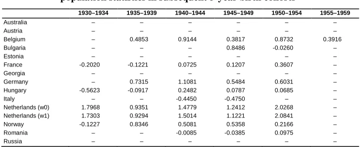
Table 4: Cohort MAFFM: mean difference between GGS estimates and population statistics in subsequent 5-year birth cohorts

1930–1934 1935–1939 1940–1944 1945–1949 1950–1954 1955–1959

Australia – – – – – –

Austria – – – – – –

Belgium – 0.4853 0.9144 0.3817 0.8732 0.3916

Bulgaria – – – 0.8486 -0.0260 –

Estonia – – – – – –

France -0.2020 -0.1221 0.0725 0.1207 0.3607 –

Georgia – – – – – –

Germany – 0.7315 1.1081 0.5484 0.6031 –

Hungary -0.5623 -0.0917 0.2482 0.0787 0.0685 –

Italy – – -0.4450 -0.4750 – –

Netherlands (w0) 1.7968 0.9351 1.4779 1.2412 2.0268 – Netherlands (w1) 1.7303 0.9294 1.5014 1.1221 2.0841 –

Norway -0.1227 0.8346 0.5081 0.5358 0.2166 –

Romania – – -0.0085 -0.0385 0.0975 –

Russia – – – – – –

The analysis of the cohort MAFFM excludes Australia, Estonia, Georgia, and Russia, as population statistics on the cohort MAFFM were not available for these countries. For France, Belgium, Bulgaria, Germany, Hungary, Italy, Norway, and Romania, the GGS estimates of the cohort MAFFM show accurate approximations of population statistics without substantial deviation (<1 year). In the Netherlands the GGS overestimates the cohort MAFFM for nearly all cohorts, with deviations ranging up to 2.08 years (Table 4).

In sum, the GGS estimates of the cohort MAFFM provide a closer approximation of population statistics than is the case for GGS estimates of the cohort TFFMR. As a result, the time-series of cohort MAFFM estimated from the GGS show significant positive correlations with the MAFFM drawn from population statistics (Table 3). Considering the results for both the cohort TFFMR and the cohort MAFFM, we can conclude that the cohort nuptiality data in the GGS are fairly accurate for cohorts born after 1940–1945, notwithstanding exceptions in a limited number of countries (see summary indicators and detailed country results in the appendix).

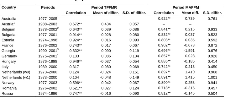
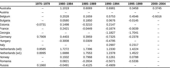
4.2 Period total female first-marriage rate and mean age at female first marriage

(29)

GGS approximate population statistics more closely. Consistent with the findings for the cohort TFFMR, however, an underestimation of first-marriage intensities is found in earlier periods for a number of countries. This underestimation mainly occurs in the late 1970s (the Netherlands and Russia in Table 6) and 1980s (Bulgaria and the Netherlands). For these countries the underestimation of the period TFFMR in earlier periods is generally below -0.05, as shown in Figure 8 for Hungary and Figure 9 for Russia. The Netherlands is exceptional, as the deviation in the period TFFMR is on average -0.16 during the 1970s. In Austria, Belgium, Germany, Italy, and the Netherlands the GGS overestimates period first-marriage intensities in the 1990s and the 2000s, with the bias being particularly pronounced in Germany (ranging up to +0.12 on average in the period 1995–1999). In Belgium and Italy, overestimations of the period TFFMR ranging up to +0.10 on average are found after 1995. Countries where the GGS estimates provide fairly accurate approximations of population statistics are Estonia (Figure 7), Georgia, Norway, and Romania. Despite variation in data quality across countries, the GGS-based period TFFMR in most countries shows significant positive correlations with time-series drawn from population statistics, indicating that the GGS accurately represent period trends in first-marriage intensities in these countries.

(30)

Figure 6: Period total female first-marriage rate, Belgium, 1970–2005

Source: Generations & Gender Survey Belgium (Wave 1), Calculations by authors.

Figure 7: Period total female first-marriage rate, Estonia, 1970–2002

(31)

Figure 8: Period total female first-marriage rate, Hungary, 1970–2003

Source: Generations & Gender Survey Hungary (Wave 1), Calculations by authors.

Figure 9: Period total female first-marriage rate, Russia, 1970–2001

(32)

Table 5: Period TTFMR & period MAFFM: mean differences, standard deviation of difference and zero-order correlation between GGS estimates and population statistics

Country Periods Period TFFMR Period MAFFM

Correlation Mean of differ. S.D. of differ. Correlation Mean diff. S.D. differ.

Australia 1977–2005 – – – 0.922** 0.739 0.761

Austria1 1988–2003 0.672** 0.434 0.057 – –

Belgium 1978–20022

0.643** 0.039 0.086 0.841** 0.215 0.933 Bulgaria 1977–2001 0.914** -0.028 0.080 0.832** 0.037 0.523 Estonia 1974–1998 0.924** 0.016 0.093 0.803** 0.035 0.592 France 1976–2002 0.743** 0.017 0.067 0.902** -0.073 0.872 Georgia 1990–20013

0.832** 0.090 0.119 0.696** -1.591 0.676 Germany 1975–20014

0.133 0.086 0.134 0.857** 0.028 0.926 Hungary 1976–1998 0.946** -0.037 0.054 0.886** -0.185 0.414 Italy 1989–2000 0.317 0.080 0.069 0.742** 0.213 0.450 Netherlands (w0) 1973–2000 0.124 -0.024 0.151 0.897** 1.410 0.968 Netherlands (w1) 1973–2000 0.104 -0.048 0.149 0.891** 1.415 1.001 Norway 1977–2003 0.596** 0.042 0.067 0.890** 0.253 0.941 Romania 1976–2002 0.621** 0.027 0.124 0.718** -0.315 0.457 Russia 1974–1996 0.747** -0.016 0.090 0.812** -0.146 0.504

Note: Significance levels: not significant (–), p < .05 (*), p < .01 (**).

1

for Austria rates between the ages 15 and 24 based on the GGS are compared to rates from vital statistics for the same age range.

2

due to availability of external data the analysis period of the Period MAFFM deviates (1978–2004).

3

4

Table 6: Period total female first-marriage rate (calculated up to age 49): mean difference between GGS estimates and population statistics in subsequent 5-year intervals

1975–1979 1980–1984 1985–1989 1990–1994 1995–1999

Australia – – – – –

Austria1

– – – 0.0674 -0.0101

Belgium – 0.0258 0.0108 0.0097 0.1094

Bulgaria – -0.0281 -0.0519 0.0376 0.0281

Estonia 0.0094 0.0173 0.0166 -0.0141 –

France – 0.0608 0.0243 -0.0061 0.0636

Georgia – – – 0.1109 0.0604

Germany 0.0115 0.0616 0.0480 0.0799 0.1225

Hungary – -0.0291 -0.0414 -0.0303 –

Italy – – – 0.0725 0.1016

Netherlands (w0) -0.1385 -0.0638 -0.0865 0.0031 0.1806 Netherlands (w1) -0.1630 -0.0843 -0.1023 -0.0116 0.1392

Norway – 0.0310 0.0708 0.0370 0.0411

Romania – -0.0225 0.1047 0.0480 0.0775

Russia -0.0184 -0.0199 0.0000 -0.0497 –

Note: 1

(33)

Table 7: Period MAFFM (calculated up to age 49): mean difference between GGS estimates and population statistics in subsequent 5-year intervals.

1975–1979 1980–1984 1985–1989 1990–1994 1995–1999 2000–2004

Australia – 1.1019 0.6069 0.6981 0.3458 0.3745

Austria – – – – – –

Belgium – 0.2028 0.1659 0.5753 0.4546 -0.6016

Bulgaria – 0.0580 0.1850 0.0676 -0.0145 –

Estonia -0.0731 0.1498 -0.3210 0.2147 – –

France – 0.2421 -0.0449 -0.1674 -0.0039 –

Georgia – – – -1.1827 -1.7041 –

Germany 0.7909 0.4403 0.3959 -0.7325 -0.2378 –

Hungary – -0.3008 0.0309 -0.4795 – –

Italy – – – 0.2997 0.2317 –

Norway – 0.1932 0.7968 0.1261 0.0788 –

Romania – 0.0821 -0.2834 -0.5071 -0.5336 –

Russia 0.1960 -0.0491 -0.4125 -0.4909 – –

Source: Generations & Gender Survey (Wave 1), Calculations by authors

4.3 Cohort total fertility rate and mean age at childbearing

(34)

For Belgium, Bulgaria, Estonia, Russia, and Romania similar conclusions can only be drawn for later cohorts (e.g., after 1945).

Population statistics on the cohort MAC are available for Australia, Belgium, Bulgaria, Estonia, France, Germany, Hungary, Italy, the Netherlands, Norway, Romania, and Russia. No results can be presented for Austria and Georgia. For Bulgaria, Estonia, France, Hungary, Norway, Romania, and Russia, the GGS estimates of the cohort MAC do not deviate substantially from population statistics (Table 10). For Belgium and Germany the GGS estimates overestimate the cohort MAC up to 1 year for the birth cohorts between 1945–1950 and 1945–1955. In Australia and the Netherlands the GGS overestimate mean ages at childbearing for all cohorts considered. In Australia the deviation between both series ranges up to 3 years in specific years, whereas deviations are generally smaller in the Netherlands, with deviations generally being limited to 1 year. In Italy the GGS substantially underestimates the cohort MAC for cohorts born in the 1940s. In sum, the GGS estimates provide a better approximation of long-term trends in the cohort MAC than is the case for the cohort TFR. As a result, for most countries significant positive correlations are found between GGS estimates of the cohort MAC and population statistics (Table 8). This is not the case, however, for the entire range of cohorts in Estonia, Italy, and Russia. In these countries, positive and significant correlations only emerge for cohorts born after 1945, indicating that the GGS more accurately reflect trends in the cohort MAC for the more recent birth cohorts.

Figure 10: Cohort total fertility rate, Australia, 1925–1965

(35)

Figure 11: Cohort total fertility rate, Netherlands, 1925–1965

Source: Generations & Gender Survey Netherlands (Wave 1), Calculations by authors.

Figure 12: Cohort total fertility rate, Romania, 1926–1965

(36)

Figure 13: Cohort total fertility rate, Russia, 1925–1965

Source: Generations & Gender Survey Russia (Wave 1), Calculations by authors.

Table 8: Cohort TFR & Cohort MAC: mean difference, and standard deviation of difference and zero-order correlation between GGS estimates and population statistics

Country Cohorts Cohort TFR Cohort MAC

Correlation Mean Diff. St. Dev. Diff. Correlation Mean Diff. St. Dev. Diff.

Australia 1930–1957 0.759** 0.004 0.258 0.393** 1.277 0.914

Austria – – – – – – –

Belgium 1930–1960 0.106 -0.227 0.286 0.689** 0.497 0.596 Bulgaria 1930–1954 -0.307 -0.340 0.136 0.667** 0.458 0.479 Estonia 1944–1955 0.227 0.038 0.117 -0.072 0.489 0.491 France 1930–1955 0.808** -0.106 0.217 0.667** 0.008 0.473

Georgia 1935–1953 0.480* -0.250 0.124 – – –

Germany 1930–1955 0.600** -0.239 0.182 0.598** 0.484 0.714 Hungary 1930–1955 -0.100 -0.157 0.110 0.419* 0.029 0.420 Italy 1939–1953 0.753** -0.196 0.107 0.290 -0.282 0.555 Netherlands (w0) 1930–1954 0.816** 0.113 0.189 0.783** 0.731 0.579 Netherlands (w1) 1930–1954 0.819** 0.090 0.191 0.814** 0.668 0.534 Norway 1930–1958 0.792** -0.088 0.132 0.832** 0.251 0.504 Romania1

1930–19551

0.385 -0.406 0.159 0.812** 0.199 0.446 Russia 1937–1954 -0.046 -0.073 0.158 0.111 0.200 0.796

1

due to limited availability of data from external sources, the data quality assesment of the cohort MAC refers to the period 1934−1958.

(37)

Table 9: Cohort TFR (calculated up to age 49): mean difference between GGS estimates and population statistics in subsequent 5-year birth cohorts

1930–1934 1935–1939 1940–1944 1945–1949 1950–1954 1955–1959

Australia -0.0259 -0.2051 0.3599 -0.0422 -0.0270 –

Austria – – – – – –

Belgium -0.4259 -0.4618 -0.2543 -0.2036 -0.0606 0.0111 Bulgaria -0.4324 -0.3907 -0.3471 -0.2767 -0.2509 –

Estonia – – – 0.0330 0.0768 –

France 0.1468 -0.0238 -0.1090 -0.0632 -0.0891 –

Georgia – -0.3127 -0.2344 -0.2755 – –

Germany -0.4446 -0.2209 -0.1724 -0.2721 -0.1428 – Hungary -0.2553 -0.2485 -0.0849 -0.1290 -0.0797 –

Italy – – -0.1728 -0.2200 -0.2295 –

Netherlands (w0) 0.0521 0.1281 0.1012 0.2060 0.0781 – Netherlands (w1) 0.0290 0.1165 0.1020 0.1588 0.0459 – Norway -0.0864 -0.1651 -0.1890 -0.0592 -0.0172 – Romania -0.5984 -0.3821 -0.4324 -0.3956 -0.3212 –

Russia – – -0.1582 -0.0012 0.0196 –

Table 10: Cohort MAC (calculated up to age 49): mean difference between GGS estimates and population statistics in subsequent 5-year birth-cohorts

1930–1934 1935–1939 1940–1944 1945–1949 1950–1954 1955–1959

Australia 1.1359 1.2771 1.0566 0.8828 – –

Austria – – – – – –

Belgium 0.4856 0.3273 0.4750 0.8843 0.3859 0.3865

Bulgaria 0.6129 0.2964 0.4847 0.6221 0.2717 –

Estonia – – – 0.3680 0.6088 –

France -0.1607 -0.0227 0.1258 0.0389 0.0274 –

Georgia – – – – – –

Germany 0.1056 0.2455 0.2518 0.9129 0.7283 –

Hungary 0.0037 -0.3247 0.4168 0.0989 -0.0964 –

Italy – – -0.7394 -0.2280 0.4742 –

Norway 0.2858 0.1020 0.0259 0.5467 0.0833 0.4468

Romania – 0.2573 -0.0588 0.2536 0.5243 –

Russia – – 0.4205 0.0804 0.3021 –

(38)

4.4 Period total fertility rate and mean age at childbearing

For all countries included in the analysis, population statistics provide time series of the period TFR, making it possible to assess the quality of GGS estimates. The results for the GGS-based period TFR show that, similar to the results for nuptiality, period indicators for fertility show smaller deviations from population statistics than cohort fertility indicators. Consistent with findings regarding cohort indicators, which particularly show underestimations of fertility in older cohorts, underestimations of the period TFR typically occur in the earliest periods considered. In the late 1970s and the 1980s, Bulgaria, Georgia, Estonia, the Netherlands, and Romania show clear underestimations of the period TFR (Table 12). Results for Bulgaria in Figure 15 and Georgia in Figure 17 are examples in this respect. In more recent periods the GGS tends to overestimate the period TFR in some countries, similar to overestimations found for period TFFMR. This overestimation of period fertility indicators is particularly noticeable during the 1990s in Georgia and Germany (up to +0.5 children per woman) and at the turn of the millennium in Belgium (up to +0.2 children per woman in selected years). Countries that do not show substantial periods of under or overestimation of fertility are Australia, Belgium, France (Figure 16), Hungary, Italy, Norway, and Russia. Also, the period TFR drawn from the Austrian GGS data (Figure 14) shows no substantial deviations, notwithstanding the limited time scope of the analysis.

Figure 14: Period total fertility rate, Austria, 1988–2005

(39)

Figure 15: Period total fertility rate, Bulgaria, 1970–2001

Source: Generations & Gender Survey Bulgaria (Wave 1), Calculations by authors.

Figure 16: Period total fertility rate, France, 1970–2005

(40)

Figure 17: Period total fertility rate, Georgia, 1970–2005

Source: Generations & Gender Survey Georgia (Wave 1), Calculations by authors.

Table 11: Period TFR & Period MAC: mean difference, standard deviation of difference and zero-order correlation between GGS estimates and population statistics

Country Periods Period TFR Period MAC

Correlation Mean of differ. S.D. of differ. Correlation Mean of differ. S.D. of differ.

Australia 1970–2005 0.808** 0.053 0.205 0.668** 0.504 1.293 Austria1

1988–2005 0.748** -0.061 0.076 0.453– 0.469 0.312 Belgium 1978–2005 0.699** 0.048 0.128 0.923** 0.312 0.375 Bulgaria 1977–2001 0.851** -0.091 0.203 0.451* 0.370 0.459 Estonia 1974–1998 0.940** -0.198 0.124 0.517** 0.324 0.418 France 1976–2002 0.365– -0.025 0.134 0.925** 0.036 0.457 Georgia 1976–2003 0.555** 0.051 0.330 0.519** -0.188 0.524 Germany 1975–2002 0.040– 0.130 0.191 0.841** 0.032 0.512 Hungary 1976–1998 0.897** -0.007 0.102 0.934** 0.016 0.265 Italy 1989–2000 0.087– -0.013 0.085 0.847** 0.338 0.360 Netherlands (w0) 1973–2000 0.229– 0.188 0.197 0.923** 0.605 0.439 Netherlands (w1) 1973–2000 0.244– 0.132 0.183 0.937** 0.590 0.419 Norway 1977–2003 0.622** 0.018 0.135 0.951** 0.080 0.309 Romania 1976–2002 0.891** -0.118 0.271 0.621** 0.125 0.405 Russia 1974–2001 0.946** 0.045 0.130 0.863** -0.149 0.425

1