A Comparative Approximate Economic Behavior
Analysis of Support Vector Machines and Neural
Networks Models
Amin Gharipour∗ Morteza Sameti∗∗ Ali Yousefian∗∗∗
Abstract
he application of the artificial neural networks in economics and business goes back to 1950s, while the main part of the applications has been developed in more recent years. Reviewing this research indicates that the development and applications of neural network are not limited to a specific application area as it spans a wide variety of fields from prediction to classification, as most of the applications in economics primarily focus on the predictive power of the neural networks. Many researches using statistical and Neural Networks (NNs) models in economics but few involved support vector machines in their studies. In this paper for the first time we compare the approximate economic behavior ability of artificial neural networks (ANN) and support vector machines using a set of data on some Middle East countries.
Keywords: Artificial Neural Networks, Forecasting, Support Vector Machines, Gross Domestic Product (GDP).
∗ Mathematical Science Dep., University of Isfahan, of Technology, Isfahan, Iran.
∗∗ Economic Dep., University of Isfahan, Iran.
1- Introduction
The neural networks are available tools for economists to estimate, predict and forecast economic variables. If modeling economic data does not require any specification of certain functional forms or exact form of functions are not know, the neural networks are good alternatives to the existing tools. Within the field of economics, econometrics, times series analysis and forecasting, finance and macroeconomics are the areas increasingly benefiting the neural networks.
Latest advances in statistics, computational learning theory, generalization theory; machine learning and complexity have presented new guidelines and deep perceptions into the general traits and nature of the model building/learning/fitting process [49]. Many of the new computational and machine learning methods generalize the idea of parameter estimation in statistics. Among these new methods, Support Vector Machines have fascinated most attention in the last few years. The aim of this paper is to compare the approximate economic behavior ability of artificial neural networks (ANN) and support vector machines.
The rest of the paper is the paper is organized as follows. Section 2 reviews the literature on GDP forecasting and application of neural networks to the economic problems. Section 3 presents the data set and data pre-processing. In section 4 we consider the problem of small size of data. Section 5 presents the models and discusses the results of the empirical application in detail. Section 6 concludes.
2- A review of literature
This section introduces the background to forecasting GDP and the application of neural networks to the economic problems.
2-1- Forecasting GDP
Adaptive Network-based Fuzzy Inference System (ANFIS) in estimating and predicting GDP.
C.S chumacher and J. Breitung (2008) discussed a factor model for short-term forecasting of GDP growth using a large number of monthly and quarterly time series in real-time. To take into account the different periodicities of the data and missing observations at the end of the sample, the factors are estimated by applying an EM algorithm, combined with a principal components estimator. They discussed some in-sample properties of the estimator in a real-time environment and proposed alternative methods for forecasting quarterly GDP with monthly factors.
Duo Qin et al (2008) compared the predict performance of Automatic Leading Indicators (ALIs) and Macro Econometric Structural Models (MESMs) commonly used by non-academic macroeconomists. Inflation and GDP growth form the forecast objects for comparison, by using data from China, Indonesia and the Philippines. R. Golinelli and G.Parigi used real-time data to mimic real-real-time GDP forecasting activity. Through automatic searches for the best indicators for predicting GDP one and four steps ahead, they compared the out-of-sample forecasting performance of adaptive models using different data vintages.
M. Marcellino (2008) provided a wide evaluation of the role of sophisticated nonlinear time series models for GDP growth and inflation. His main conclusion is that in general linear time series models can be scarcely beaten if they are carefully specified, and therefore still provide a good benchmark for theoretical models of growth and inflation. He also identified some important cases where the adoption of a more complicated benchmark can alter the conclusions of economic analyses about the driving forces of GDP growth and inflation. Therefore, comparing theoretical models also with more sophisticated time series benchmarks can guarantee more robust conclusions.
Union, and Euro area). BM forecasting ability is always better to that of benchmark models, provided that at least some monthly indicator data are available over the forecasting horizon.
M. Diron (2008) proposed to evaluate the contributions of three sources of forecast error using a set of data vintages for the euro area. Diron’s results showed that gains in accuracy of forecasts achieved by using monthly data on actual activity rather than surveys or financial indicators are offset by the fact that the former set of monthly data is harder to forecast and less timely than the latter set. These results provide a benchmark which future research may build on as more vintage datasets become available.
C. Schumacher (2007) in “Forecasting German GDP Using Alternative Factor Models Based on Large Datasets” discussed the forecasting performance of alternative factor models based on a large panel of quarterly time series for the German economy. One model extracts factors by static principal components analysis; the second model is based on dynamic principal components obtained using frequency domain methods; the third model is based on subspace algorithms for state space models. Out-of-sample forecasts showed that the forecast errors of the factor models are on average smaller than the errors of a simple autoregressive benchmark model. Among the factor models, the dynamic principal component model and the subspace factor model outperform the static factor model in most cases in terms of mean-squared forecast error.
In another area addressing GDP prediction, Tkacz (2001) used neural networks to find out more exact leading indicator models of Canadian output growth by analyzing the forecast performance of multivariate neural networks and finding that there are gains in the short-run forecast precision of the neural networks in comparison to the best linear model due to the neural networks’ ability to capture non-linear relationships in the data.
2-2- Background of Artificial Neural Networks in Economy
M. Sameti et al (2009) compared two forecasting macroeconomic time series models, neural networks with dynamic architecture and feed forward neural network that is a useful neural network approach for macroeconomic time series prediction and demonstrated that the networks with dynamic architecture and internal memory like Elman neural network out perform feed forward neural network in estimate and predicting Iran and Turkey GDP.
Heravi, Osborn, and Birchenhall (2004) employed neural networks and linear patterns to forecast seasonally unadjusted monthly real industrial production data of important sectors of German, French and UK economies. They compared the forecast performance of the neural networks with linear models and found that while linear models outperform the neural networks up to a year forecasts, the neural networks perform better than the linear models in predicting the direction of change. Nakamura (2005) assessed the usefulness of neural networks in inflation forecasting and found that the neural networks outperform univariate autoregressive models in predicting short-horizon of one and two quarters inflation rates.
The neural networks can be also useful tools in mapping and estimation problems in microeconomics. B. C. Erbas And S. E. Stefanou construct a Multilayer Feed-forward Neural Network (MFNN) with back-propagation and found that multilayer feed-forward neural network can be used in calculating electricity output for the given inputs in this sub-sector of the US electricity market, and these estimations can be employed in policy design and planning.
existing tools in measuring technical efficiency. Similarly, Delgado (2005) employed the neural networks for efficiency analysis in public sector, refuse collection services, and found that it was useful to employ the neural networks as complementary tools in efficiency analysis.
Kuan and Liu (1995) used feed-forward and recurrent neural networks to scrutinize nonlinear models in exchange rates and test the performance of the selected networks in forecasting. In addition to the aforementioned researches, the neural networks are used in few other areas such as identifying market structures (Gruca & Klemz, 1998), and estimating marketing margins (Mainland, 1998), productivity analysis (Boussabaine & Duff, 1996).
The major bulk of the studies on neural networks have focused on accounting and finance problems, with special emphasis on credit evaluation, bankruptcy forecasting, swindle revealing, assets evaluation, etc. Neural networks have been widely applied to tackle problems arising from the financial and economical areas (see Vellido, Lisboa, & Vaughan (1999) for an overview). We can classify neural networks applications to these areas as works tackling the following problems.
Classification and discrimination: In this kind of problems the net must determine which class an input pattern belongs to. Classes are either user-defined (in classification problems) or run-time grasped by the net itself (similarly to the cluster-analysis (Wooldridge, 2002)). The main problem to be tackled is the credit risk assessment, but other problems exist: Bank failure prediction (Tam & Kiang, 1992), stocks classification (Kryzanowsky, Galler, & Wright, 1993), etc.
Function approximation and optimization: This class consists of problems that can not be said to belong to the previous two classes. Examples are given by portfolio selection and re-balancing (Fernandez & Gomez, 2005; Steiner & Wittkemper, 1997; Zimmermann & Neuneier, 1999) and investment project return prediction (Badiru & Sieger, 1998).
3- The data set and pre-processing
For our experiments, we used data of 200 financial indicators from a World Bank data set. data mining, also known as ‘‘knowledge discovery in databases”, is the process of discovering meaningful forms in large databases (Han & Kamber, 2001) the DM basic operations include ‘data clean’ and ‘data reduction’: In the ‘data clean’ process, we remove the noise data, or reply to the missing data field. In the ‘data reduction’ process, we decrease the unnecessary dimensionality or adopt useful transformation methods. The primary objective is to improve the effective number of variables under consideration.
3-1- Data clean
Missing data poses problems when performing data analysis. Complete and precise data are necessary in obtaining good inference. There are applications which need missing data to be approximated.
There are mainly 3 types of missing data: Missing At Random (MAR), Missing Not At Random (MNAR) and Missing Completely At Random (MCAR). MAR is when the missing data is dependant on other variable in the dataset. In other words, an incorrect data for a variable can be the cause of another variable’s data to be missing. The missing data pattern is traceable in MAR. MNAR is when missing data is dependant on other missing data in the dataset and is un-ignorable. MCAR is when the missing data has no dependence on other variable/s or even to it self. Data is simply “just missing” and no relation can be derived between variables to find out the cause of the missing data.
There are mainly two approaches to missing data. If there are few records with missing data deleting missing data is plausible but in this research we have many missing data, so the second approach, estimating the missing data is the more plausible approach because the ANN requires certain amount of data to train.
3-2- Data reduction
Salcedo-Sanz, DePrado-Cumplido, Segovia-Vargas,Pe´rez-Cruz, & Bouson˜o-Calzo´ n, 2004; Tahai, Walczak, &Rigsby, 1998). These approaches can be classified into three types: feature selection, feature extraction, and feature construction (Liu & Motoda, 1998). Feature extraction projects a high-dimension feature space to a low-dimension space via linear/non-linear transformations such that most of the information in the original features is retained. Feature selection includes selecting a ‘‘good” subset of features that save the most useful information for a given task. Feature extraction and feature construction involve finding a set of ‘‘composite” features, which are functions of the original features. Feature construction addresses the problem of feature interaction by discovering good combinations of the original features. Many past studies have adopted a data-driven approach and focused on automating the process of searching for the best representation of input features (e.g., Langley & Sage 1994; Matheus & Rendell, 1989; Pakath & Zaveri 1995; Piramuthu et al. 1998; Ragavan et al. 1993; Tahai et al.1998). A number of studies have combined feature-preprocessing algorithms with classification methods to improve their performance. For example, West (1985) extended a log it model by preprocessing features with factor analysis.
3-2-1- Future extraction
The most popular statistical method for dimensionality reduction of a large data set is the Karhunen-Loeve (K-L) method, also called Principal Component Analysis (PCA). Principal component analysis is a method of transforming the initial data set represented by vector samples into a new set of vector samples with derived dimensions. The goal of this transformation is to concentrate the information about the differences between samples into a small number of dimensions. More formally, the basic idea can be described as follows:
1. Firstly the data set procured from the experiment are normalized as
)) ( min( )) ( max(
)) ( min( ) ( ) (
j x j
x
j x j x j
x i
i −
− =
′ (1)
2. The new normalized multi-response array for m parameters and n experiment can be represented by matrix x′as
⎥ ⎥ ⎥ ⎥ ⎦ ⎤ ⎢ ⎢ ⎢ ⎢ ⎣ ⎡ ′ ′ ′ ′ ′ ′ ′ = ′ ) ( ) 2 ( ) 1 ( . . . ) ( . . . ) ( ) 2 ( ) 1 ( 2 1 1 1 m x x x m x m x x x x n n n L M L (2)
3. The correlation coefficient array (Rjl) of matrix x′is written as Follows ) ( ) ( )) ( ), ( cov( l x j x i i jl i i l x j x R ′ ′ × ′ ′ = σ
σ , j=1,2,L,m , l=1,2,L,m (3)
Where cov(x′i(j),x′i(l))is the covariance of sequences xi′(j) and )
(l xi′ ; x(l)
i
′
σ is the standard deviation of sequence xi′(l).
4. The eigenvalues and eigenvectors of matrix (Rjl) are calculated.
5. The PC are computed as follows
∑
= × ′ = m j k ii k x j v j p 1 ) ( ) ( )
( (4)
Where pi(k) is the kth PC corresponding to ith experiment, vk(j) is jth element of kth eigenvector.
6. The total principal component index (TPCI) corresponding to ith experiment (pi) is computed as follows
∑
= × = m k ii p k e k
p
1
) ( )
( (5)
∑
= = m k k eig k eig k e 1 ) ( ) ( )( (6)
Where eig(k) is the kth eigenvalue.
3-2-2- Feature selection
Real-world datasets often contain a large number of features some of which are either redundant or irrelevant to the given tasks (Fayyad, Piatetsky-Shapiro, & Smyth, 1996). This happens when it is unknown which features are related to a target concept and especially when domain knowledge is unavailable or incomplete. Many features are then introduced to represent an unknown domain. The existence of irrelevant and redundant features may make vague the distribution of really relevant features for a target concept and hence cause damage the models (John, Kohavi, & Pfleger, 1994; Koller & Sahami, 1996; Ragavan, Rendell, Shaw, & Tessmer, 1993). In addition, increasing the dimensionality of the feature space will generally result in increased complexity of interactions among the features and increased degree of noise. In this study we used Parallel Genetic Algorithm for feature Selection.
Let C={x1,x2,K,xp} be the set containing all of p possible features, and
Ω
be the collection of all subsets of C, The goal of feature selection is to find, in some sense, the “best”ω
∈Ω. Finding the “best”ω
∈Ω is a typical combinatorial optimization problem. There are altogether 2p−1 nontrivial subsets of C. An interesting heuristic search algorithm well suited for the combinatorial optimization problem is the genetic algorithm.Genetic Algorithm is a stochastic optimization technique invented by Holland (1975) and a search algorithm based on survival of the fittest among string structures (Goldberg, 1989). The idea of GAs is to get “better solutions” using “good solutions”, and the algorithm process is as follows:
1. Solution representation: For problems that require real number solutions, a simple binary representation is used where unique binary integers are mapped onto some range of the real line. Each bit is called a gene and this binary representation is called chromosome. Once a representation is chosen, the GA proceeds as follows: A large initial population of random candidate solutions is generated. These are then continually transformed following steps 2 and 3.
2. Select the best and eliminate the worst solution on the basis of a fitness criterion (e.g., higher the better for a maximization problem) to generate the next population of candidate solutions.
(a) Crossover: A pair of binary integers (chromosomes) is split at a random position and the head of one is combined with the tail of other and vice-versa.
(b) Mutation:The state (0 or 1) of a randomly chosen bit is changed. This helps the search avoid being trapped into local optima.
4. Repeat steps (2) and (3) until some convergence criterion is met or some fixed number of generations has passed.
In 2006 Mu Zhu and Hugh A. Chipmanfirst demonstrated that the GA, although perfectly natural for the variable selection problem, is actually not easy to use or terribly effective and then proposed a very simple modification. Their idea is to run a number of GAs in parallel without allowing each GA to fully converge, and to unify the information from all the individual GAs in the end. They called the resulting algorithm the parallel genetic algorithm (PGA). They showed with a methodical simulation study that parallel evolution or PGA is competitive in its ability to recover the correct model. They also illustrated the strength and usefulness of parallel evolution with both simulated and real datasets and indicate its general ability to be implemented as a feature selection tool for more complex statistical models. The PGA is a stochastic search method. In this regard, it is similar to SSVS, and they are both better than greedy stepwise methods but the PGA is somewhat more accessible and easier to use than SSVS in practice because the success of SSVS is deeply dependent on being able to select the correct set of prior parameters.
4-The problem of small size of data
When the data set is small, over fitting becomes an important problem so different techniques have been proposed to avoid the problem of over fitting. In this paper we used Cubic spline interpolation to increase the number of observation for each variable and after that using validation method to solve the problem of over fitting.
4-1- Cubic spline interpolation
Interpolation is used to estimate the value of a function between known data points without knowing the actual function. In each case, the approach to this problem is to assume that whatever is being measured moves in a smooth and continuous way, and to use the data available annually (or quarterly) to make the best guess about what the values of a quarterly (or monthly) series should be.
Cubic spline interpolation is a useful technique to interpolate between known data points because of, it's steady and smooth characteristics. Spline theory is simple. Over n intervals, the usual fits n equations subject to the boundary conditions of n+1 data points. The derivations of Lilley and Wheatly [39,40] are used. The derivation assumes a functional form for the curve fit. This equation form is simplified and then solved for the curve fit equation. The assumed form for the cubic polynomial curve fit for each segment is, i i i i i i
i x x b x x c x x d
a
y= ( − )3+ ( − )2+ ( − )+
(7)
where the spacing between successive data points is
i i
i x x
h = +1− (8)
The cubic spline constrains the function value, 1st derivative and 2nd derivative. The routine must ensure that y(x), y¢(x) and y¢(x) are equal at the interior node points for adjacent segments.
Substituting a variable S for the polynomial’s second derivative reduces the number of equations from a, b, c, d for each segment to only S for each segment.
For the ith segment, the S governing equation is,
⎟⎟ ⎠ ⎞ ⎜⎜ ⎝ ⎛ − − − = + + + − − + + − − − 1 1 1 1 1 1
1 (2 2 ) 6
i i i i i i i i i i i i i h y y h y y s h s h h s
h (9)
In matrix form, the governing equations reduce to a tri-diagonal form.
⎥ ⎥ ⎥ ⎥ ⎥ ⎦ ⎤ ⎢ ⎢ ⎢ ⎢ ⎢ ⎣ ⎡ − − − − − − = ⎥ ⎥ ⎥ ⎥ ⎦ ⎤ ⎢ ⎢ ⎢ ⎢ ⎣ ⎡ ⎥ ⎥ ⎥ ⎥ ⎦ ⎤ ⎢ ⎢ ⎢ ⎢ ⎣ ⎡ + + + − − − − − − − − − − 2 2 1 1 1 1 1 2 2 2 3 1 2 1 2 2 2 3 2 2 2 2 1 6 ) ( 2 ) ( 2 ) ( 2 n n n n n n n i n n n n h y y h y y h y y h y y S S S h h h h h h h h h h M M O O
O (10)
1
equations. Finally, the cubic spline properties are found by substituting into the following equations.
a, b, c and d values correspond to the polynomial definition for each segment.
i i i
i s s h
a =( +1− )/6 (11)
2 /
i
i s
b = (12)
6
2 1
1 +
+ − −
= i i
i i i i
S h h
y y
c (13)
i i y
d = (14)
4-2- Validation
Validation is performed to avoid the problem of overfitting (Smith, 2002). When a network is over-trained, it memorizes the training examples. While overtraining results in very small errors in training set, it results in large errors when the network is tested with the new data. In other words, the network can not generalize successfully.
In order to improve generalization, validation enables early stopping. In order to validate, at the very start, the data is grouped into three subsets; training set, validation set and test set. The training set is used to train the network by computing weights and errors, while the validation set is to cross-check the training process. This is done by observing the patterns in validation errors. The training is stopped, when the validation errors increases for a specified number of iterations. On the other hand, the test set is used for checking the performance of the network in generalization.
5- Model
5-1- Artificial neural network (ANN)
usually depending on the task the network has to learn. Usually, the network topology is kept constant, but in some applications the topology itself can be considered as a parameter and can dynamically change. The most used network topologies are the following:
• layered,
• Completely connected
Networks of the first category have neurons subdivided in layers. If the connections are only in one direction (i.e., each neuron receives inputs from the previous layer and sends output to the following layer), they are called feed forward networks. Otherwise, if also ‘loops’ are allowed, the network is called recurrent network. Completely connected networks, on the other hand, have neurons which are all connected with each other.
The feed forward neural networks are the most popular architectures due to their structural flexibility, good representational capabilities and availability of a large number of training algorithms. This network consists of neurons arranged inlayers in which every neuron is connected to all neurons of the next layer (a fully connected network).
MLP and RBF networks are two kinds of feed forward neural network with different transfer functions. Note that according to Hornic and Kreinovich [2] using a feedforward ANN with one hidden layer, every bounded continuous function can be approximated with arbitrarily small error. An output of a three-layer MLP networks is defined by
∑
∑
= =
+ + =
1
1 1
2 1 1 1 2 2
2 ( ( ) )
s
j
R
i
k j i ij jk
k f w f w p b b
a , k=1,...,s2 (15)
Fig1: Multilayer Perceptron Network
synaptic weight parameter and bias, respectively. There are some choices for the transfer function f which can be globally supported.
Linear : f
( )
x =x (16)Log – sigmoid:
( )
x e xf −
+ =
1
1 (17)
Tan – sigmoid:
( )
1 12
2 − + = − x
e x
f (18)
Positive linear: f
( )
x =x if x≥0 , f( )
x =0 if x<0 (19) In order to approximate functionψ
(x1,x2,...,xR) where) ,..., ,
(x1 x2 xR are R independent input variables, a three layer perceptron network with R input neurons, S1hidden neurons by tan-sigmoid transfer function and one output neuron by linear transfer function are selected. So, we can write as follows:
∑
∑
= =
+ + ≈
1
1 1
2 1 1 1 1 2
1, ,..., ) ( )
(
s
j
R
j
k j i jk jk
R w f w x b b
x x x
ψ (20)
Where w and b are the unknown coefficient.
The desirable neural network architecture is constructed by experimenting with different structures. Since there is no defined regulation for determining the number of hidden layers, it is necessary to go through a trial and error process (Kuan&White, 1992). During the experimentation phase the neural network builder needs to guard against the consequences of using either very few or too many nodes in hidden layers. When only a few nodes are used, there might be a problem of under-identification of nonlinearity. When too many nodes are used there may be a problem of over identification where the network memorizes the pattern in the training data and performs poorly in the generalization data.
5-2- Support Vector Machines
machine, a novel neural network algorithm, was developed by Vapnik and his colleagues [50]. It is on the basis of the Structural Risk Minimization principle from computational learning theory. Hearst et al. [50] positioned the SVM algorithm at the intersection of learning theory and practice: ‘‘it contains a large class of neural networks, Radial Basis Function (RBF) nets, and polynomial classifiers as special cases. Yet it is simple enough to be analyzed mathematically, because it can be shown to correspond to a linear method in a high dimensional feature space nonlinearly related to input space.’’ A simple description of the SVM algorithm is presented here, for more details please refer to Refs. [43, 44, 51, 52].
5-2-1- Basic concepts
We define a training data set D={(x1,y1),K,(xN,yN)} where R
y X
xi∈ , i∈ , N is the number of training data points, and X denotes the space of the input samples Rn. SVMs are linear learning machines which means that a linear function (f(x)=wTx+b) is always used to solve the regression problem. The best line is defined to be that line which minimizes the following cost function (Q):
∑
=+
+ N
i i i b
w
C w
i
i 1
* 1
, , ,
) (
min
*ξ ξ
ξ ξ
(21)
s.t. ( T i ) i,
i w x b y − + ≤ε+ξ (wTxi+b)− yi ≤
ε
+ξ
i*, i 0, i 0,i 1, ,N*
K
= ≥ ≥ ξ ξ
Where
ξ
iandξ
i* are the corresponding positive and negative errors at the ith point, respectively.minimization with constraints. This can be solved by applying Lagrangian theory.
5-3- Measuring error
The difference between the actual output and the network output is called error. There are several ways of measuring error including; Normalized Mean Squared Error (NMSE), Mean Absolute Error (MAE), Mean Squared Error (MSE), we used MAE to measure the error and, therefore, the performance of the network, in Eq. (22)
∑
=
− = Q
k k k y
y Q MAE
1
ˆ
1 (22)
Where Q is the number of observations in the data set.
6- Experimental result
In this investigation, the Gaussian function is used as the kernel function of SVMs, which is inspired by the empirical findings that Gaussian kernels tend to give good performance under general smoothness assumptions, and therefore should be considered especially if no additional knowledge of the data is available. As there is no structured way to choose the optimal parameters of SVMs, the values of the kernel parameter δ2, C
and
ε
that produce the best result on the validation set are used for the standard SVMs.In terms of using artificial neural network we implement Multilayer Perceptron Network with three layer, 21 neurons in input layer 28 neurons in hidden layer by tan-sigmoid transfer function for predict Middle East GDP.
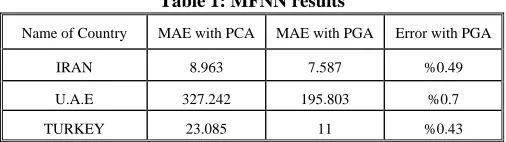
Table 1: MFNN results
Error with PGA MAE with PGA
MAE with PCA Name of Country
%0.49 7.587
8.963 IRAN
%0.7 195.803
327.242 U.A.E
%0.43 11
Table 2: SVM results
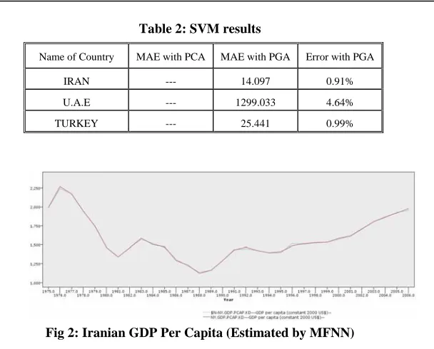
Fig 2: Iranian GDP Per Capita (Estimated by MFNN)
Fig 3: U.A.E GDP Per Capita (Estimated by MFNN)
Fig 4: Turkey GDP Per Capita (Estimated by MFNN)
Error with PGA MAE with PGA
MAE with PCA Name of Country
0.91% 14.097
--- IRAN
4.64% 1299.033
--- U.A.E
0.99% 25.441
7- Conclusions
Decision makers in different parts of the economic (business, government, the central bank, financial markets, etc) activate in real-time and establish their choices on an early comprehending of the state of economic Activity, usually measured by key macroeconomics variable GDP because this is the most frequently quoted and monitored macroeconomic indicator of an economy.
In this paper for the first time we compared the approximate economic behavior ability of artificial neural networks (ANN) and support vector machines (SVM) model using a set of data on some Middle East countries.
The results showed that neural network out perform support vector machines in both terms of generalization from training data set and accuracy of approximation.
References
1- A. Gharipour, A. Yousefian, M. Sameti, Economic Herd Behavior in Some Middle East Countries Evaluationof Artificial Neural Networks Approach for Prediction, Proceedings of 2009 International Conference on Economics, Business Management and Marketing, Singapore, 9-11 October, 2009.
2- B. C. Erbas, S. E. Stefanou, An application of neural networks in microeconomics: Input–output mapping in a power generation subsector of the US electricity industry, Expert Systems with Applications 36 (2009) 2317–2326.
3- Bastianoni, S., Pulselli, F. M., Focardi, S., Tiezzi, E. B. P., & Gramatica, P. (2008). Correlations and complementarities in data and methods through principal component analysis (PCA) applied to the results of the SPIn – Eco Project. Journal of Environmental Management, 86, 419– 426.
4- C. O’Neill, Cubic Spline Interpolation, not published (2002).
5- C. Schumacher, Forecasting German GDP Using Alternative Factor Models Based on Large Datasets, J. Forecast. 26, 271–302 (2007).
6- C. Schumacher, Forecasting German GDP Using Alternative Factor Models Based on Large Datasets, J. Forecast. 26, 271–302 (2007).
A.Cologni, M. Manera, The asymmetric effects of oil shocks on output growth: A Markov–Switching analysis for the G-7 countries, Economic Modelling (2008).
8- D. Qin, M. A. Cagas, G. Ducanes, N. M.Ramos, P. Quising, Automatic leading indicators versus macroeconometric structural models: A comparison of inflation and GDP growth forecasting, International Journal of Forecasting 24 (2008) 399–413.
9- Dubey, A. K., & Yadava, V. (2008). Multi-objective optimization of Nd: YAG laser cutting of nickel-based superalloy sheet using orthogonal array with principal component analysis. Optics and Lasers in Engineering, 46, 124–132.
10-E. Anderson, Travel And Communication And International Differences In GDP Per Capita, J. Int. Dev. 19, 315–332 (2007).
11-E. Angelini, G. di Tollo, A. Roli, A neural network approach for credit risk evaluation, The Quarterly Review of Economics and Finance, 48 (2008) 733–755.
12-H. LI, L. HUANG, Health, education, and economic growth in China: Empirical findings and implications, China Economic Review (2008).
13-H. Li, Y. Gao, A GDP fluctuation model based on interacting firms, Physica A 387 (2008) 5225–5230
14-J. Galindo, P. Tamayo, Credit risk assessment using statistical and machine learning: basic methodology and risk modeling applications, Computational Economics 15 (1 – 2) (2000)107–143.
15-J. Pons, The Accuracy of IMF and OECD Forecasts for G7 Countries, J. Forecast. 19, 53-63 (2000).
16-K.-Jae Kim, Financial time series forecasting using support vector machines, Neurocomputing 55 (2003) 307 – 319.
17-K.M.Hornik, M.Stinchcombe, H.White, Multilayer Feed forward networks are universal approximators, Neural networks , 2,1989,pp.359366.
18-K.-R. Mu¨ller, S. Mika, G. Ratsch, K. Tsuda, B. Scho¨lkopf, An introduction to kernel-based learning algorithms, IEEE Transactions on Neural Networks 12 (2) (2001) 181– 201.
A.Karami, Estimation of the critical clearing time using MLP and RBF neural networks, Euro. Trans. Electr. Power (2008).
20-L. Yu, S. Wang a, K.K. Lai, Forecasting crude oil price with an EMD-based neural network ensemble learning paradigm, Energy Economics 30 (2008) 2623–2635.
21-M. Ashiya, Strategic Bias and Professional Affiliations of Macroeconomic Forecasters, J. Forecast. (2008).
22-M. Ashiya, Strategic Bias and Professional Affiliations of Macroeconomic Forecasters, J. Forecast. (2008).
23-M. Diron, Short-Term Forecasts of Euro Area Real GDP Growth: An Assessment of Real-Time Performance Based on Vintage Data, J. Forecast. 27, 371–390 (2008).
24-M. Diron, Short-Term Forecasts of Euro Area Real GDP Growth: An Assessment of Real-Time Performance Based on Vintage Data, J. Forecast. 27, 371–390 (2008).
25-M. Marcellino, A Linear Benchmark for Forecasting GDP Growth and Inflation?, J. Forecast. 27, 305–340 (2008).
26-M. Marcellino, A Linear Benchmark for Forecasting GDP Growth and Inflation?, J. Forecast. 27, 305–340 (2008).
27-M. McAleera, M.C. Medeiros, D. Slottje, A neural network demand system with heteroskedastic errors, Journal of Econometrics 147 (2008) 359 -371.
28-M. Paliwal, U. A. Kumar, Neural networks and statistical techniques: A review of applications, Expert Systems with Applications 36 (2009) 2–17.
29-M. Sameti, A. Yousefian, A. Gharipour, Economic Herd Behavior in Iran and Turkish Evaluation of Artificial Neural Networks with Dynamic Architecture, Proceedings of 2009 International Conference on Economics, Business Management and Marketing, Singapore, 9-11 October, 2009.
30-M.A. Hearst, S.T. Dumais, E. Osman, J. Platt, B. Scho¨lkopf, Support vector machines, IEEE Intelligent Systems 13 (4) (1998) 18– 28.
A.Mandal, K. Johnson, Sequential Elimination of Level Combinations by Means of Modified Genetic Algorithms, not published.
31-Mu Zhu, H. A. Chipman, Darwinian Evolution in Parallel Universes: A Parallel Genetic Algorithm for Variable Selection, Technometrics, 48, 491-502.
32-N. Cristianini, J. Shawe-Taylor, An Introduction to Support Vector Machines, Cambridge Univ. Press, Cambridge, New York, 2000.
33-R. Golinelli, G. Parigi, Real-time squared: A real-time data set for real-time GDP forecasting, International Journal of Forecasting 24 (2008) 368–385.
34-R. Golinelli, G. Parigi, The Use of Monthly Indicators to Forecast Quarterly GDP in the Short Run: An Application to the G7 Countries, J. Forecast. 26, 77–94 (2007).
35-R. Golinelli, G. Parigi, The Use of Monthly Indicators to Forecast Quarterly GDP in the Short Run: An Application to the G7 Countries, J. Forecast. 26, 77–94 (2007).
36-R.S. Bartholo, C.A.N. Cosenza, F.A. Doria, C.T.R. de Lessa, Can economic systems be seen as computing devices?, Journal of Economic Behavior & Organization (2008).
37-RO´ Mulo A. Chumacero, Empirical Analysis of Systematic Errors in Chilean GDP Forecasts, J Forecast 19\ 26 34 (1990).
38-Roger E. A. Farmer, A. Lahiri, Economic Growth in an Interdependent World Economy, The Economic Journal, 116 (2006), 969–990.
39-S. Eickmeier, C. Ziegler, How Successful are Dynamic Factor Models at Forecasting Output and Inflation? A Meta-Analytic Approach, J. Forecast. 27, 237–265 (2008).
40-S.M.Taheri,K.Mahdaviani,J.Mohammadi , Modeling Semi Linear Relations with small size of data using artificial neural networks,J.Information Science &Applications volume 3,November 2256_2261(2008).
41-U. Çaydas, A. Hasçalık, S. Ekici, An adaptive neuro-fuzzy inference system (ANFIS) model for wire-EDM. Journal of Expert Systems with Applications 36 (2009) 6135–6139.
42-U. Thissen, R. van Brakel, A.P. de Weijer, W.J. Melssen, L.M.C. Buydens, Using support vector machines for time series prediction, Chemometrics and Intelligent Laboratory Systems 69 (2003) 35– 49.
44-V.Y.Kreinovich, Arbitrary nonlinearity is sufficient to represent all functions by neural networks: A Theorem, Neural Networks,4 ,1991,pp.381-383.
45-W.S. Chen, Y.K. Du, Using neural networks and data mining techniques for the financial distress prediction model, Expert Systems with Applications 36 (2009) 4075–4086.
46-Y. Shirvany, M. Hayati, R. Moradian, Multilayer perceptron neural networks with novel unsupervised training method for numerical solution of the partial differential equations, Applied Soft Computing 9 (2009) 20–29.
47-Y. Shirvany, M. Hayati, R. Moradian, Multilayer perceptron neural networks with novel unsupervised training method for numerical solution of the partial differential equations, Applied Soft Computing 9 (2009) 20–29.
48-Y.H. Wang, Nonlinear neural network forecasting model for stock index option price: Hybrid GJR–GARCH approach, Expert Systems with Applications 36 (2009) 564–570.