R E S E A R C H
Open Access
Stability estimate and regularization for a
radially symmetric inverse heat conduction
problem
Wei Cheng
**Correspondence:
[email protected] College of Science, Henan University of Technology, Zhengzhou, 450001, P.R. China
Abstract
This paper investigates a radially symmetric inverse heat conduction problem, which determines the internal surface temperature distribution of the hollow sphere from measured data at the fixed location inside it. This is an inverse and ill-posed problem. A conditional stability estimate is given on its solution by using Hölder’s inequality. A wavelet regularization method is proposed to recover the stability of solution, and the technique is based on the dual least squares method and Shannon wavelet. A quite sharp error estimate between the approximate solution and the exact ones is obtained by choosing a suitable regularization parameter.
MSC: 65M30; 35R30; 35R25
Keywords: inverse heat conduction; ill-posed problems; stability estimate; regularization; error estimate
1 Introduction
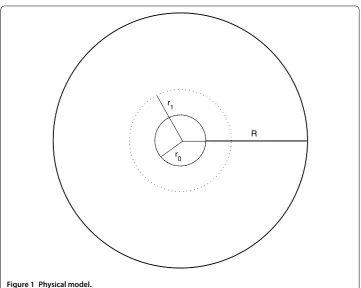
A physical model considered here is a hollow sphere, andRandrdenote its external and
internal radius, respectively. Let the hollow sphere be adiabatic at its external surface, and a thermocouple is installed inside the hollow sphere at the radiusr=r, r<r<R, as
illustrated in Figure . Assuming a spherically symmetric temperature distribution of the model, the correspondingly mathematical model can be described as the following radially symmetric heat conduction problem:
ut=urr+
rur, r<r<R,t> ,
u(r, ) = , r≤r≤R,
u(r,t) =g(t), t≥,
ur(R,t) = , t≥,
(.)
whererdenotes the radial coordinate,g(t) is the temperature history at one fixed radius
r,r<r<R. We want to recover the temperature distributionu(r,·) (r≤r<r) based
on the measured data ofg(·). This is an inverse heat conduction problem.
The inverse heat conduction problem (IHCP) has numerous important applications in various sciences and engineering []. For example, determination of thermal fields at
Figure 1 Physical model.
faces without access, obtaining the force applied to a complex structure from knowledge of the response and transfer function which describes the system, or the diagnosis of a disease by computerized tomography []. In all cases, the boundary conditions of these problems are inaccessible to measurements or not known. Usually sensors are installed beneath the surface and the unknown boundary conditions of these problems are esti-mated.
inves-tigated the determination of spatially- and temperature- dependent thermal conductivity by a semi-discretization method. In this work, we will use a wavelet method to deal with IHCP (.) (r≤r<r) with variable coefficient and to obtain a quite sharp error estimate
between the approximate solution and the exact solution.
The wavelet method has become a powerful method for solving partial differential equa-tions (PDEs). And the method has been applied to direct problems as well as to various types of inverse problems such as the IHCP [], the Cauchy problem of Laplace equation [, ], the backward heat conduction problem [], the inverse source identification problems [, ] and the Cauchy problem for the modified Helmholtz equation [, ]. It is worth mentioning that Feng and Ning [] used a Meyer wavelet regularization method for solving numerical analytic continuation and presented the Hölder-type stability es-timates. In this paper, we solve the radially symmetric inverse heat conduction problem (.) in the interval [r,r) by determining the temperature distribution using a wavelet
dual least squares method generated by the family of Shannon wavelets.
When we deal with problem (.) inL(R) with respect to variablet, we extend all
func-tions of variabletappearing in the paper to be zero fort< . Since the measurement data ofg(t) contain noises, the solutions have to be sought from the data functiongδ(t)∈L(R),
which satisfy
g–gδ≤δ, (.)
where the constantδ> denotes a bound on the measurement error, and · represents theL(R) norm. It is also assumed that there exists an a priori bound for functionu(r
,t)
u(r,·)Hp≤E, p≥, (.)
whereu(r,·)Hpdenotes the norm in the Sobolev spaceHp(R) defined by u(r,·)Hp:=
∞
–∞
+ξpfˆ(ξ)dξ
.
Using the Fourier transform with respect to the variablet, problem (.) can be formulated in a frequency space as follows:
⎧ ⎪ ⎪ ⎨ ⎪ ⎪ ⎩
iξuˆ(r,ξ) =∂∂ruˆ(r,ξ)+r ∂uˆ(r,ξ)
∂r , r∈(r,R],ξ∈R, ˆ
u(r,ξ) =gˆ(ξ), ξ∈R,
ˆ
ur(R,ξ) = , ξ∈R.
(.)
We can get a formal solution for problem (.), refer to [],
ˆ
u(r,ξ) = (r/r)ϕ(r,ξ)e(r–r)
√
iξgˆ(ξ), r∈[r
,R),ξ∈R, (.)
where
ϕ(r,ξ) = ( √
According to Lemma . in [], functionϕ(r,ξ) satisfies
c≤ϕ(r,ξ)≤c, r∈[r,r),ξ∈R, (.)
wherecandcare positive constants. Due to|(r/r)ϕ(r,ξ)e(r–r)
√
iξ|increases rapidly with
exponential order as|ξ| → ∞, the Fourier transform of the exact datag(t) must decay rapidly at high frequencies forr>r. But such a decay is not likely to occur ingδ(t). So, a
small measurement error in the given datagδ(t) in high frequency components can com-pletely destroy the solution of problem (.) forr∈[r,r).
For problem (.), we define an operatorAr:u(r,·) −→g(·) in the spaceX=L(R). Then problem (.) can be rewritten as
Aru(r,t) =g(t), ∀u(r,·)∈X,r≤r<r. (.)
According to expression (.), there holds
Aru(r,ξ) =gˆ(ξ) = (r/r)e(r–r)
√
iξϕ–(r,ξ)uˆ(r,ξ), r∈[r
,r). (.)
Then we have Aru(r,ξ) :=Aruˆ(r,ξ) and a multiplication operator Ar:L(R) −→L(R) given by
Aruˆ(r,ξ) = (r/r)e(r–r)
√
iξϕ–(r,ξ)uˆ(r,ξ). (.)
Therefore, we have the following lemma.
Lemma . If A∗r is the adjoint of Ar,then A∗r corresponds to the following problem:
⎧ ⎪ ⎪ ⎪ ⎪ ⎪ ⎨ ⎪ ⎪ ⎪ ⎪ ⎪ ⎩
–∂U∂t =∂∂rU +r∂U∂r, r<r≤R,t≥,
U(r, ) = , r≤r≤R,
U(r,t) =g(t), t≥,
Ur(R,t) = , t≥,
(.)
and
A∗r= (r/r)e(r–r)
√
iξϕ–(r,ξ). (.)
Proof Using the following relations and expression (.)
Aru,υ=Aruˆ,υˆ=
ˆ
u,Ar
∗
ˆ
υ=u,A∗rυ=uˆ,A∗rυˆ,
where·,·denotes the inner product, we can obtain the adjoint operatorA∗r ofArin the frequency domain
A∗r=Ar
∗
= (r/r)e(r–r)
√
Applying the Fourier transform with respect to the variablet, we can rewrite problem (.) in the following form (in the frequency space):
⎧ ⎪ ⎪ ⎨ ⎪ ⎪ ⎩
–iξUˆ(r,ξ) =∂∂rUˆ(r,ξ)+r ∂Uˆ(r,ξ)
∂r , r∈(r,R],ξ∈R, ˆ
U(r,ξ) =gˆ(ξ), ξ∈R,
| ˆUr(R,ξ)|= , ξ∈R.
(.)
Taking the conjugate operator for problem (.), we know thatUˆ(r,ξ) =uˆ(r,ξ). So, com-bining with (.), we get
ˆ
U(r,ξ) =uˆ(r,ξ) = (r/r)e(r–r)
√
iξϕ(r,ξ)gˆ(ξ) (.)
and
ˆ
g(ξ) = (r/r)e(r–r)
√
iξϕ–(r,ξ)Uˆ(r,ξ) =A∗
rUˆ(r,ξ) =A∗rU. (.)
The outline of the paper is as follows. In Section , using Hölder’s inequality, we prove the conditional stability for IHCP (.) in the interval [r,r). The relevant properties of
Shannon wavelets are summarized in Section . The last section presents error estimates via wavelet dual least squares method approximation.
2 A conditional stability estimate
In this section, we give a conditional stability in the following theorem.
Theorem . Let u(r,t)be the exact solution of problem(.)given by(.)and the a priori bound(.)hold.Then,for a fixed r∈(r,r),we have the following estimate:
u(r,·)≤c(c)
r–r r–r(r/r)
r–r
r–ru(r,·) r–r r–rg
r–r
r–r, (.)
where cand care constants given by(.).
Proof Using Parseval’s formula, expression (.) and Hölder’s inequality, we have
u(r,·)=uˆ(r,·)= ∞
–∞
(r/r)ϕ(r,ξ)e(r–r)
√
iξgˆ(ξ) dξ
= ∞
–∞
(r/r)ϕ(r,ξ)
(r–r)
r–r e(r–r)√iξgˆ(ξ) r–r
r–rgˆ(ξ) r–r r–r dξ
≤
∞
–∞
(r/r)ϕ(r,ξ)
(r–r)
r–r e(r–r)√iξgˆ(ξ) dξ
r–r r–r ∞
–∞
gˆ(ξ)dξ r–r
r–r
=
∞
–∞
(r/r)ϕ(r,ξ)
(r–r) r–r (r
/r)ϕ(r,ξ)
–
ˆ
u(r,ξ)
dξ r–r
r–r g
(r–r) r–r
≤sup
ξ∈R
(r/r)ϕ(r,ξ)
(r/r)ϕ(r,ξ)
(r–r) r–ruˆ(r
,·)
(r–r) r–rg
From inequalities (.), we get
(r/r)ϕ(r,ξ)(r/r)ϕ(r,ξ)
(r–r) r–r ≤(r
/r)c
(r/r)c
(r–r) r–r .
Then there holds
u(r,·)≤c(c)
(r–r) r–r(r/r)
(r–r)
r–r u(r,·) (r–r)
r–rg(r–rr–r) .
The conclusion of Theorem . is proved.
Remark . Ifu(r,t) andu(r,t) are the solutions of problem (.) with the exact data g(t) andg(t), respectively, then for a fixedr∈(r,r), there holds
u(r,·) –u(r,·)≤Cu(r,·) –u(r,·)
r–r r–rg
(·) –g(·)
r–r
r–r, (.)
where C=c(c)
r–r r–r(r/r)
r–r
r–r. It is obvious that ifg(·) –g(·) →, thenu(r,·) –
u(r,·)forr<r≤r.
In the next section, the relevant properties of Shannon wavelets are summarized.
3 The Shannon wavelets
Suppose thatφandψare the Shannon scaling and wavelet functions whose Fourier trans-forms are given by
ˆ φ(ξ) =
⎧ ⎨ ⎩
, |ξ| ≤π,
, otherwise, (.)
and
ˆ ψ(ξ) =
⎧ ⎨ ⎩
e–iξ, π≤ |ξ| ≤π,
, otherwise. (.)
Letφj,k(t) :=
j
φ(jt–k),ψj,k(t) := j
ψ(jt–k),j,k∈Z,–,k:=φ,kandl,k:=ψl,kfor
l≥, the index set
˜
I={j,k}:j,k∈Z⊂Z, ˜
IJ=
{j,k}:j= –, , . . . ,J– ;k∈Z⊂Z.
Then the subspacesVJ can be defined
VJ=span{λ}λ∈˜IJ (.)
and an orthogonal projectionPJ:L(R) −→VJ:
PJϕ=
λ∈˜IJ
We have, for anyk∈Z,
supp(ψˆj,k) =
ξ:πj≤ |ξ| ≤πj+, (.)
supp(φˆj,k) =
ξ:|ξ| ≤πj. (.)
Expression (.) shows thatPJ can be considered as a low pass filter.
4 Regularization and error estimates
In this section, the wavelet dual least squares method will be described and error estimates be given by Theorems .-..
4.1 Dual least squares method
We now introduce the dual least squares method for approximation of the solutions of problem (.). For the operator equationAu=g, a general projection method is generated by two subspace families {Vj}and{Yj} ofX. Then the approximate solutionuj∈Vj is defined to be the solution of the following problem:
Auj,y=g,y, ∀y∈Yj. (.)
IfVj⊂R(A∗) and subspacesYjare chosen in such a way that
A∗Yj=Vj,
then there is a special case of projection method known as the dual least squares method. Suppose that{ψλ}λ∈˜Ij is an orthogonal basis ofVjandyλis the solution of the equation
A∗yλ=kλψλ, yλ= . (.)
Then we can obtain the approximate solution
uj=
λ∈˜Ij g,yλ
kλ
ψλ. (.)
According to (.), we easily concludeuJ=PJu. In order to give an error estimate for the regularized solution, we need a sequence of subspacesYjapproximating the spaceXand contained in the range ofA∗. FromA∗Yj=Vj, the subspacesYjare spanned bywλ,λ∈ ˜IJ, where
A∗wλ=λ and kλ=wλ–, yλ=
wλ wλ
=kλwλ. (.)
We know thatwλis a solution of the following problem (see Lemma .):
⎧ ⎪ ⎪ ⎪ ⎪ ⎪ ⎨ ⎪ ⎪ ⎪ ⎪ ⎪ ⎩
–∂U∂t =∂U
∂r +r∂U∂r, r<r≤R,t≥, U(r, ) = , r≤r≤R,
U(r,t) =j,k(t), t≥,
Ur(R,t) = , t≥.
Becausesuppψˆj,k is compact, the solution exists for anyt∈(,∞). Analogously, the so-lution of the adjoint equation is unique. So, for givenλ,wλcan be uniquely determined according to (.). From (.), there holds
ˆ
wλ=
r re
(r–r)√iξϕ(r,ξ)ˆλ(ξ), λ={j,k}, (.)
combining with (.), we have
ˆ
yλ=
r re
(r–r)√iξϕ(r,ξ)k
λˆλ(ξ), λ={j,k}. (.)
Thus we have the approximate solution for noisy datagδgiven by
PJuδ(r,t) =uδJ =
λ∈˜IJ
uδ,λ
λ=
λ∈˜IJ
gδ,yλ
kλ
λ. (.)
4.2 Error estimates
We estimate firstly the errorsPJu–PJuδandu–PJuby Theorems . and ., respec-tively.
Theorem .(Stability) Let PJu(r,t)given by(.)and PJuδ(r,t)given by(.)be the
reg-ularized approximate solutions to u(r,t)for the data g and gδ,respectively.If the measured
data gδ(t)satisfy condition(.),then for any fixed r∈[r
,r),we have
PJu–PJuδ≤(cr/r)e(r–r)
√
πJδ. (.)
Proof Due to (.), (.) and (.), for any fixedr∈[r,r), there holds
PJu(r,·) –PJuδ(r,·)=
λ∈˜IJ
g–gδ,y λ
kλ λ
=
λ∈˜IJ
ˆ
g–gδ,yˆ λ
kλ ˆ λ
=
λ∈˜IJ
ˆ
g–gδ,r
re
(r–r)√iξϕ(r,ξ)k λˆλ
kλ ˆ λ
≤ sup
πJ–≤|ξ|≤πJ
(r/r)e(r–r)
√
iξϕ(r,ξ)·
λ∈˜IJ
ˆ
g–gδ,ˆ λ
ˆ λ
≤ sup
πJ–≤|ξ|≤πJ
(r/r)e(r–r)
√
iξϕ(r,ξ)·Pˆ J
ˆ
g–gδ,
combining with inequality (.) and condition (.),
PJu(r,·) –PJuδ(r,·)≤(cr/r) sup
πJ–≤|ξ|≤πJ
e(r–r)√|ξ|/δ
≤(cr/r)e(r–r)
√
Theorem .(Convergence) If u(r,t)is the solution of problem(.)satisfying the a priori
condition(.),then for any fixed r∈[r,r),we have
u(r,·) –PJu(r,·)≤(c/c)
J+–pe(r–r)
√
πJE. (.)
Proof According to (.), we get
u(r,·) = λ
u(r,·),λ
λ,
PJu(r,·) =
λ∈˜IJ
u(r,·),λ
λ.
By using Parseval’s relation and (.), (.), (.), there holds
u(r,·) –PJu(r,·)
=uˆ(r,·) –PJu(r,·)=
λ∈˜I
ˆu,ˆλ ˆλ–
λ∈˜IJ
ˆu,ˆλ ˆλ
=
λ∈˜Ij≥J+
ˆu,ˆλ ˆλ
= λ∈˜Ij≥J+
(r/r)ϕ(r,·)e(r–r)
√
i(·)gˆ(·),ˆ
λ ˆ λ =
λ∈˜Ij≥J+
(r/r)ϕ(r,·)ϕ–(r,·)e(r–r)
√
i(·)uˆ(r ,·),ˆλ
ˆ λ
≤ sup
πJ≤|ξ|≤πJ+
rϕ(r,ξ) rϕ(r,ξ)
e(r–r)√iξ|ξ|–p
λ∈˜Ij≥J+
+ (·)p/uˆ(r,·),ˆλ ˆ
λ
≤ sup
πJ≤|ξ|≤πJ+
(c/c)|ξ|–pe(r–r)
√
|ξ|/E≤(c /c)
J+–pe(r–r)√πJE.
We have proved estimate (.).
Theorem . Let u(r,t)be the exact solution of(.)and PJuδgiven by(.)be the
regu-larized approximate solution to u(r,t).If the measured data gδ(t)satisfies condition(.)
and the a priori condition(.)is valid when we select
J=log
π
r–r ln E δ lnE δ
–p
, (.)
then for any fixed r∈[r,r),we have
u(r,·) –PJuδ(r,·)
≤E–
r–r r–rδ
r–r r–r
lnE
δ
–p(–r–r r–r)
C+o() forδ→, (.)
Proof From Theorem . , Theorem . and the choice rule (.) ofJ, we can get
u(r,·) –PJuδ(r,·)
≤(c/c)
J+–pe(r–r)
√
πJE+ (cr/r)e(r–r) √
πJδ
≤(c/c)E(r–r)p
ln
E
δ
lnE
δ
–p–p E
δ
lnE
δ
–pr–r r–r
+ (cr/r)δ
E
δ
lnE
δ
–pr–r r–r
≤E–
r–r r–rδ
r–r r–r
lnE
δ
–p(–r–r r–r) c
((r–r)lnEδ)
p
c(ln(Eδ(lnEδ)–p))p
+cr
r
.
Note that
lnE δ
ln(Eδ(lnEδ)–p)=
lnE δ
lnEδ – pln(lnEδ)→ forδ→.
We have obtained estimate (.).
Remark .
(i) Ifp= andr<r<r, estimate (.) becomes
u(r,·) –PJuδ(r,·)≤
(c/c) + (cr/r)
E–
r–r r–rδ
r–r
r–r, (.)
which is a Hölder stability estimate.
(ii) Ifp> , estimate (.) is a logarithmical-Hölder stability estimate, especially at
r=r, it becomes
u(r,·) –uδ(r,·)≤E
lnE
δ –p
C+o()→ forδ→, (.)
which is a logarithmical stability estimate.
5 Conclusion
In this paper the radially symmetric inverse heat conduction problem is considered. A con-ditional stability result is established by utilizing the a priori bound. We obtain a regular-ized solution by a wavelet dual least squares method and the error estimate of logarithmic Hölder type between the approximate solution and the exact ones by choosing a suitable regularization parameter.
Abbreviation
IHCP, inverse heat conduction problem.
Competing interests
The author declares that she has no competing interests.
Author’s contributions
Acknowledgements
The author would like to thank the anonymous referees for their valuable comments and helpful suggestions on this work. The project is supported by the National Natural Science Foundation (NNSF) of China (11561045), the Natural Science Foundation of Henan Province of China (132300410231).
Publisher’s Note
Springer Nature remains neutral with regard to jurisdictional claims in published maps and institutional affiliations.
Received: 30 November 2016 Accepted: 4 April 2017
References
1. Alifanov, OM: Inverse Heat Transfer Problems. Springer, Berlin (1994)
2. Fernandes, AP, Santos, MB, Guimarães, G: An analytical transfer function method to solve inverse heat conduction problems. Appl. Math. Model.39, 6897-6914 (2015)
3. Beck, JV, Blackwell, B, Clair, SR: Inverse Heat Conduction: Ill-Posed Problems. Wiley, New York (1985)
4. Carasso, A: Determining surface temperatures from interior observations. SIAM J. Appl. Math.42, 558-574 (1982) 5. Seidman, T, Eldén, L: An optimal filtering method for the sideways heat equation. Inverse Probl.6, 681-696 (1990) 6. Tautenhahn, U: Optimality for ill-posed problems under general source conductions. Numer. Funct. Anal. Optim.19,
377-398 (1998)
7. Murio, DA: Stable numerical evaluation of Grünwald-Letnikov fractional derivatives applied to a fractional IHCP. Inverse Probl. Sci. Eng.17(2), 229-243 (2009)
8. Garshasbi, M, Dastour, H: Estimation of unknown boundary functions in an inverse heat conduction problem using a mollified marching scheme. Numer. Algorithms68(4), 769-790 (2015)
9. Hào, DN, Thanh, PX, Lesnic, D, Johansson, BT: A boundary element method for a multi-dimensional inverse heat conduction problem. Int. J. Comput. Math.13, 1540-1554 (2012)
10. Hon, YC, Wei, T: A fundamental solution method for inverse heat conduction problem. Eng. Anal. Bound. Elem.28, 489-495 (2004)
11. Eldén, L, Berntsson, F, Regi ´nska, T: Wavelet and Fourier methods for solving the sideways heat equation. SIAM J. Sci. Comput.21(6), 2187-2205 (2000)
12. Regi ´nska, T, Eldén, L: Solving the sideways heat equation by a wavelet-Galerkin method. Inverse Probl.13, 1093-1106 (1997)
13. Regi ´nska, T, Eldén, L: Stability and convergence of wavelet-Galerkin method for the sideways heat equation. J. Inverse Ill-Posed Probl.8, 31-49 (2000)
14. Fu, CL, Qiu, CY: Wavelet and error estimation of surface heat flux. J. Comput. Appl. Math.150, 143-155 (2003) 15. Wróblewska, A, Frackowiak, A, Cialkowski, M: Regularization of the inverse heat conduction problem by the discrete
Fourier transform. Inverse Probl. Sci. Eng.24(2), 195-212 (2016)
16. Qian, Z, Zhang, Q: Differential-difference regularization for a 2D inverse heat conduction problem. Inverse Probl. 26(9), 095015 (2010)
17. Elkinsa, BS, Keyhania, M, Franke, JI: Global time method for inverse heat conduction problem. Inverse Probl. Sci. Eng. 20(5), 651-664 (2012)
18. Xiong, XT, Hon, YC: Regularization error analysis on a one-dimensional inverse heat conduction problem in multilayer domain. Inverse Probl. Sci. Eng.21(5), 865-887 (2013)
19. Chapko, R, Johansson, BT, Vavrychuk, V: A projected iterative method based on integral equations for inverse heat conduction in domains with a cut. Inverse Probl.29(6), 065003 (2013)
20. Fu, CL: Simplified Tikhonov and Fourier regularization methods on a general sideways parabolic equation. J. Comput. Appl. Math.167, 449-463 (2004)
21. Grabski, JK, Lesnic, D, Johansson, BT: Identification of a time-dependent perfusion coefficient in the bioheat equation. Int. Commun. Heat Mass Transf.75, 218-222 (2016)
22. Mierzwiczak, M, Kolodziej, JA: The determination temperature-dependent thermal conductivity as inverse steady heat conduction problem. Int. J. Heat Mass Transf.54, 790-796 (2011)
23. Chang, CL, Chang, M: Inverse determination of thermal conductivity using semi-discretization method. Appl. Math. Model.33, 1644-1655 (2009)
24. Regi ´nska, T: Application of wavelet shrinkage to solving the sideways heat equation. BIT Numer. Math.41(5), 1101-1110 (2000)
25. Vani, C, Avudainayagam, A: Regularized solution of the Cauchy problem for the Laplace equation using Meyer Wavelets. Math. Comput. Model.36, 1151-1159 (2002)
26. Qiu, CY, Fu, CL: Wavelets and regularization of the Cauchy problem for the Laplace equation. J. Math. Anal. Appl. 33(2), 1440-1447 (2008)
27. Wang, JR: Shannon wavelet regularization methods for a backward heat equation. J. Comput. Appl. Math.235(9), 3079-3085 (2011)
28. Dou, FF: Wavelet-Galerkin method for identifying an unknown source term in a heat equation. Math. Probl. Eng. 2012, Article ID 904183 (2012)
29. Qian, AL: Identifying an unknown source in the Poisson equation by a wavelet dual least square method. Bound. Value Probl.2013, 267 (2013)
30. Regi ´nska, T, Wakulicz, A: Wavelet moment method for the Cauchy problem for the Helmholtz equation. J. Comput. Appl. Math.223, 218-229 (2009)
31. Dou, FF, Fu, CL: A wavelet method for the Cauchy problem for the Helmholtz equation. ISRN Appl. Math.2012, Article ID 435468 (2012)
32. Feng, XL, Ning, WT: A wavelet regularization method for solving numerical analytic continuation. Int. J. Comput. Math.92(5), 1025-1038 (2015)