Non-Linear Electromechanical System Dynamics

University of New Orleans University of New Orleans

ScholarWorks@UNO

ScholarWorks@UNO

University of New Orleans Theses and

Dissertations Dissertations and Theses

Spring 5-16-2014

Non-Linear Electromechanical System Dynamics

Non-Linear Electromechanical System Dynamics

Shathiyakkumar Ganapathy Annadurai

[email protected]

Follow this and additional works at: https://scholarworks.uno.edu/td

Part of the Controls and Control Theory Commons, Electrical and Electronics Commons, and the

Electromagnetics and Photonics Commons

Recommended Citation Recommended Citation

Ganapathy Annadurai, Shathiyakkumar, "Non-Linear Electromechanical System Dynamics" (2014). University of New Orleans Theses and Dissertations. 1799.

https://scholarworks.uno.edu/td/1799

This Thesis is protected by copyright and/or related rights. It has been brought to you by ScholarWorks@UNO with permission from the rights-holder(s). You are free to use this Thesis in any way that is permitted by the copyright and related rights legislation that applies to your use. For other uses you need to obtain permission from the rights-holder(s) directly, unless additional rights are indicated by a Creative Commons license in the record and/or on the work itself.

Non-Linear Electromechanical System Dynamics

A Thesis

Submitted to the Graduate faculty of the University of New Orleans

In partial fulfillment of the Requirements for the degree of

Master of Science In

Engineering

Naval Architecture & Marine Engineering

By

Shathiyakkumar Ganapathy Annadurai B.E. Marine Engineering, Anna University, 2007

ii

Dedicated to

iii

Acknowledgement

I wish to express my heartfelt thanks to all the people who supported me during the

composition of this work. I have learned many new and exciting things, and for whichI

would like to especially thank Dr Nikolaos Xiros for guiding me throughout the thesis

and making me complete by instilling so much confidence. I would like to thank God and

iv

Table of Contents

List of figures ... vii

Nomenclature...ix

Abstract ...xi

1 Introduction ... 1

1.1 Objective ... 1

1.2 Applications Overview ... 1

1.2.1 Energy Harvesting ... 1

1.2.2 Vibration Analysis & Vibration Control ... 1

1.3 Text Outline ... 3

1.4 Context of Thesis ... 3

1.5 Description of Systems ... 4

1.6 Model Description ... 4

1.6.1 Single magnet model ... 4

1.6.2 Two – Magnet Model ... 5

1.7 Uncoupled System Dynamics ... 7

1.7.1 Mechanical Subsystem ... 7

1.7.2 Electrical system ... 7

1.8 Coupled system dynamics ... 8

1.8.1 Low-pass equivalent system ... 11

v

1.8.3 Limiters for single magnet system ... 16

2 Two Magnet systems ... 26

2.1.1 Two- Magnet model Governing Equations ... 26

2.1.2 Two Magnet Description ... 26

2.1.3 Limiters for two magnet system ... 27

3 Two Magnet, Band-Pass System ... 29

3.1 Model Description ... 29

3.2 System Equations ... 29

3.3 Results of Band- pass system under different conditions ... 30

3.3.1 Systems displacement of mass ... 30

3.3.2 Systems current ... 32

4 Two Magnet, Low-Pass system ... 34

4.1 Systems Equations ... 34

4.2 Model testing under same condition as Band-pass ... 36

4.2.1 Displacement of the system ... 36

4.2.2 Current Envelope ... 37

5 Two Magnet, Low-Pass Perturbation System ... 39

5.1 Model description ... 39

5.2 Governing Equations of Right Magnet ... 39

5.2.1 Mechanical Subsystem ... 39

5.2.2 Electrical Subsystem ... 40

vi

5.3.1 Displacement of the mechanical subsystem:... 45

5.3.2 Current Envelope ... 46

6 Validation of Low-Pass Equivalent & Low-pass Perturb Models ... 48

6.1 Description ... 48

6.2 Condition 1 ... 48

6.2.1 Right Magnet Real Parts ... 49

6.3 Condition 2 ... 50

6.4 Condition 3 ... 52

7 Conclusion ... 55

References ... 57

Appendix A ... 59

Mechanical subsystem... 59

Electrical subsystem-LP ... 60

Electrical Subsystem-BP ... 61

vii

List of figures

Figure 1- One Magnet Model ... 5

Figure 2- two magnet model ... 6

Figure 3- Band-pass & Low-pass Flat Line validations ... 19

Figure 4- Monochromatic Disturbance- of amplitude 1.0cos5t N ... 20

Figure 5- Polychromatic disturbance ... 22

Figure 6- displacement comparison for low-pass (green) and band-pass(blue) ... 23

Figure 7- Displacement and imaginary current envelope comparison... 24

Figure 8- limiter check ... 25

Figure 9- Two Magnet Model... 28

Figure 10- displacement ... 31

Figure 11-Right Magnet Current ... 32

Figure 12-Left Magnet Current ... 32

Figure 13 – Displacement LP ... 36

Figure 14- Real Part of right Magnet current envelope ... 37

Figure 15- Imaginary Part of right Magnet current envelope ... 37

Figure 16- Real Part of left Magnet current envelope ... 38

Figure 17- Imaginary Part of left Magnet current envelope ... 38

Figure 18- Displacement –LP Perturb ... 45

Figure 19- Real Part of right Magnet Current Envelope ... 46

Figure 20- Imaginary part of Right Current Envelope ... 46

Figure 21- Real part of Left Current Envelope ... 47

Figure 22- Imaginary part of Left Current Envelope ... 47

Figure 23-Zero disturbance & Zero excitation voltage ... 49

Figure 24-Zero disturbance & Zero excitation voltage ... 50

viii

Figure 26- Real right current envelope at 0.005N Monochromatic disturbance and 10V

on right magnet & 20V on left magnet. ... 53

Figure 27- Imaginary right current envelope at 0.005N Monochromatic disturbance and

10V on right magnet & 20V on left magnet. ... 54

ix

Nomenclature

Capacitance of Left EM F 5.00E-06

Capacitance of Right EM F 2.00E-05 Charge Envelope of Left EM C

Charge Envelope of Right EM C Current Envelope of left EM A Current Envelope of Right EM A

Damping b kg/s 0.25

Displacement y cm

Displacement influencing the inductance, Left

EM cm

Displacement influencing the inductance,

right EM cm

Distance between EM’s cm 10

Disturbance d N

Frequency of Left EM rad/s 2000

Frequency of Mechanical system rad/s 10

Frequency of Right EM rad/s 1000

Inductance of Left EM , H, H/m 0.05,0.5 Inductance of Right EM , H, H/m 0.05,0.5

Mass m kg 0.25

Rate of change of charge Envelope of Left EM C/s (A) Rate of change of Charge Envelope of Right

EM C/s (A)

Rate of change of current Envelope of Left EM A/s Rate of change of Current Envelope of Right

EM A/s

x Description

Notations

Used

Units,

(If applicable)

Values,

(if applicable)

Resistance of Right EM , Ω(ohms) 1 State space Matrices (), () 1/s, A/Vs (1/ Ωs)

State space vector of current and charge

envelopes , C, A

State space vector of displacement and

velocity , m, m/s

Stiffness of spring K Kg/s2 0.1

xi

Abstract

Electromechanical systems dynamics analysis is approached through non-linear

differential equations and further creating a state space model for the system. There are

three modules analyzed and validated; the first module consists two magnet coupled

with a mass spring damper system as a band-pass system; a Low-pass equivalent system

and a Low-pass equivalent system through perturbation analysis. Initially Band Pass

frameworks for the systems are formulated considering the relation between the

mechanical forcing and current. Using Mathematical tools such as the Hilbert

Transforms, a Low-Pass equivalent of the systems is derived. The state equations of the

systems are then used to design a working model in MATLAB and simulations

investigated completely.

Keywords

1

1

Introduction

1.1

Objective

The Electromechanical system is non-linearly coupled; if analyzed extensively and with

the prospective development in their controls will make to be a great tool in the field of

mechatronics for a number of applications including vibration analysis, vibration control

and energy harvesting.

1.2

Applications Overview

The vast and continuing reduction in the size and power led to focus on development of

effective tools for monitoring & control in various fields.

1.2.1 Energy Harvesting

The micro-electromechanical systems (MEMS) have been proven to be an attractive

technology for harvesting small magnitudes of energy from ambient vibrations. This

technology eliminates the need for replacing chemical batteries or complex wiring in

micro-sensors/micro-systems, moving us closer toward battery-less autonomous

sensors systems and networks. The recent year development shows that they can

provide real time information on consumption of energy. The mechanical component

vibrates due to the force induced by the ambient vibration, this movement of the

component changes the flux linked in the electric circuit in turn changing the current

envelope which could in-turn be used for the components operation.

1.2.2 Vibration Analysis & Vibration Control

Vibrations are inherent part of any system and structure which needs to be attended

continuously through-out the span of operation. This can be effectively addressed by

2

electromagnetic force created by the electrical system. The displacement of the

mechanical system can be monitored and controlled effectively. With recent

development in the self-powered MEMS, the analysis and control has improved

efficiently with remote and autonomous control and monitoring. The Vibration analysis

field is of numerous types, some types of vibration where this work on

electromechanical systems is of great use are,

1.2.2.1 Structural Vibrations

A smaller sensor reduces the strain caused by the added sensors on the structure,

preserving dynamics of structures. Smaller sensors can also be used to monitor the local

strain on structures without averaging the strain at the neighborhood. MEMS/NEMS

could be solution for the structural vibration control and monitoring.

1.2.2.2 Vortex Induced Vibrations

In fluid dynamics, vortex-induced vibrations [1] are motions induced on bodies

interacting with an external fluid flow, produced by or the motion producing periodical

irregularities on this flow. MEMS actuators have recently made their way to the

forefront of flow control research. Flow control is most effective when applied near the

transition or separation points, i.e., near the critical flow regimes where flow

instabilities amplify quickly. This is especially important for micro actuators because

these actuators cannot deliver large forces or high power. The matching in length scale

between the micro transducers and the structures makes the manipulation of these

structures possible. This phenomenon being most common in offshore structures and

underwater cables, such extension of the work proposed in this thesis will also address

3

1.3

Text Outline

The chapters following from now on will be in the outline as follows, the module one

consisting of initial chapters detailing Band-pass systems governing equation derivation

and the low-pass equivalent governing equations derived using the Hilbert transform

tool and following chapters details the validation of work done by Dr. Xiros, Associate

Professor, University of New Orleans and Mr. Psarrou. The later chapters present the

two magnet model with the developed concept of single magnet model and validation

of this system for various disturbance forms and also for different voltage profiles.

1.4

Context of Thesis

In this thesis, analysis of spectrally decoupled but non-linearly coupled subsystems is

carried out using appropriate mathematical tools. The electrical system (RLC circuit) is

evidently band-pass operating near resonant frequency while the mechanical system

which is a mass, spring & damper system operating at much lower frequency is a

low-pass subsystem. When these two systems are coupled and its dynamics analyzed by

designing a simulated model, the system has to be run at twice the frequency of the

higher frequency. This is overcome by deriving low-pass equivalent of the subsystem

describing its essential dynamics. Thus the mechanical subsystem is influenced by the

voltage source of the electric (RLC circuit), but the mechanical subsystems position also

influences the inductance of the circuit therefore presenting a mutual interaction. If

there is external disturbance the subsystems can be suitably designed to cope, thus the

objective of the system as a whole is maintained.

Both the systems are validated for different disturbance conditions and different voltage

profile. The validation of single magnet model and two magnet models carried out and

results compared and effectiveness of both discussed for further extension in the field

4

This two magnet system is used for payload positioning. The results are discussed for

future work in different applications as afore said. The band-pass system current

through resistor will be in phase with the voltage source.

The appendix at end of the report contains the Simulink coding of the systems built for

analysis.

1.5

Description of Systems

As put-forth earlier electromechanical systems comprises of two subsystems. Before

describing the systems there are few basic definitions required to better understand the

dynamics of coupled subsystems.

There are different types of Signals and Systems [2], in this thesis we will be focusing on

the linear or Non-linear time invariant systems. A linear system is any system that obeys

the properties of scaling (homogeneity) and superposition, while a non-linear system is

any system that does not obey at least one of these. The coupled subsystems exhibit

similar properties of the Non-linear time invariant systems; this will be evident as the

dynamics of the coupled subsystems will be desired.

1.6

Model Description

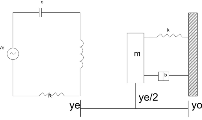
1.6.1 Single magnet model

The single magnet model [3] comprises of One RLC circuit (Band-Pass subsystem) and a

mass-spring- damper arrangement. The mass’s spring when at its natural length places

the mass at midpoint from the fixed end towards the electromagnet. The fixed end is at

y0=0 and the electromagnet is at distance of ye. Thus the mass can move from 0 to

maximum ye. The dynamics of the non-linearly coupled subsystems will be analyzed by

5

Figure 1- One Magnet Model

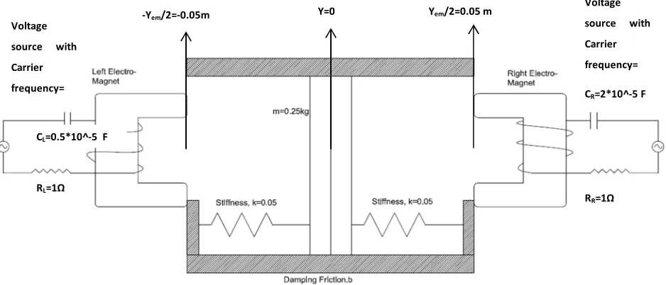
1.6.2 Two – Magnet Model

The validations and verification is made using the two magnet model, in the mass’s

spring when at its natural length is at y0=0 and the both the electromagnets are at

effective distance of ye/2. Based on these limits and already derived governing

equations of single magnet model as shown in (1-10) & (1-12), governing equations

6

Inductance of the circuit

L1234 5 L6 Lξ1234; ξ1234 5 9y 6 y2/2

L<=>?4 5 L6 Lξ<=>?4; ξ<=>?4 5 y 6 y2/2

Figure 2- two magnet model RL=1Ω

CL=0.5*10^-5 F

-Yem/2=-0.05m Y=0 Yem/2=0.05 m

Friction coeff., b=0.25 kg/sec

Voltage

source with

Carrier

frequency=

RR=1Ω CR=2*10^-5 F Voltage

source with

Carrier

7

1.7

Uncoupled System Dynamics

1.7.1 Mechanical Subsystem

Considering the mechanical subsystem as represented above Figure 1- One Magnet

Model, the second order force equation of the system can be represented as following

my 6 by 6 ky 5 fem(t) 6 d (1—1)

Where,

m--- Mass of the payload

b--- Damping coefficient

k--- Spring constant

fem (t) --- Electromagnetic force experienced by the mass

d--- Disturbance force

y--- Displacement of mass, and its corresponding velocity and acceleration.

The natural resonant frequency of the mass spring damper system is given by,

ωm5Ek/m (1—2)

1.7.2 Electrical system

The second order force equation of the electrical system can be represented as,

8 Where,

L--- Inductance,

R--- Resistance,

C--- Capacitance,

e(t) - Voltage source,

q--- Charge at the capacitor, corresponding current and rate of change of current

The resonant frequency of the RLC circuit is,

5E1/(LC) (1—4)

Thus equations represent the linear dynamics of both subsystems.

1.8

Coupled system dynamics

In this chapter, an analytical model defining the governing equations of the coupled

system will be shown [4]. The subsystem when analyzed for its dynamics separately they

are shown above, but these two systems are coupled and both are interacting with each

other.

Let’s see the electrical subsystem now, the inductance of the electromagnet a function

of the displacement of mass because the flux linkage is proportional to inductance of

the circuit. It is a clear fact that as the mass is closer to the coil the flux cut by the mass

will be more so the inductance will be higher. But as the mass is farther out of the

influence of the flux linkage there will be still a self -inductance of the coil existing.

Based on this basic electromagnetic theory, the inductance as a function of

displacement can be given as,

9 Where,

L0 – Self-Inductance of the coil,

L1 – Sensitivity of the coil as influenced by the displacement of the mass

Outside the limits though the flux linkage still exists it is negligible and the systems will

be decoupled, so the limits are placed.

Let’s consider the mechanical subsystem, the force influenced by the mass is from two

sources one will be the electromagnetic force and exogenous disturbance as explained

earlier. The electromotive force [5] caused by the electromagnet is given by,

fem 5 N edl (1—6)

Where

e—Voltage source

I— Current flowing through the coil,

e 5 φ, rate of change of flux (1—7)

φ 5 L(y). I, flux linkage (1—8)

Combining equation above, it can be easily found that

fem 5 (I_L

/2) (1—9)

my 6 by 6 ky 5 LY Z

10

[(\(])^)

[4 6 Rq 6

^

_5 e(t) (1—11)

(L 6 Ly)q 6 (L 6 R)q 6 q/C 5 e(t) (1—12)

Thus the above four equations clearly show the non-linearly coupled electromechanical

system. The inductance of the coil is the factor that couples the subsystems, if the L1

tends to becomes “0” the subsystems decouple. This is the governing equation which

depicts the dynamics of the systems clearly.

Electrical subsystem is Band-pass system as the natural frequency of subsystem will be

much higher than the natural frequency of the mass spring damper system. If seen little

clearly, the voltage source will be a combination of low-pass signal that is the signal

corresponding to that of the mass and band-pass signal containing the electrical system

higher frequency. This is similar to modulated signal used in signal transmission [6]. That

is the electrical signal is the carrier signal which is required for the low-pass signal to

carry out the positioning of the mass in the field of the magnetic flux.

The variables considered for representing system are displacement and velocity of the

mechanical system, while for the electrical system the charge and the current are the

variables. Thus those are the states space variables. Hence the governing equations with

these variables can be given as following,

q 5 (e(t) 9 (Ly 6 R)q 9 q/C)/(L6 Ly) (1—13)

q 5 I (1—14)

y 5 (LY Z

9 d 9 by 9 ky)/m (1—15)

11

The above equations are used to build the band-pass model representing the entire

system.

1.8.1 Low-pass equivalent system

In this chapter, a detailed description will be of given how a low-pass equivalent set of

governing equations will be derived using the Hilbert Transform. The objective is finding

an equivalent in low pass is because as “Nyquist” [7] proposed that in order to properly

reconstruct a signal, any signal, baseband or band-pass, needs to be sampled by at least

two times its highest spectral frequency. The point here is that the mathematical

concept will help us get around the signal processing requirements by Nyquist for

sampling of band-pass systems.

As earlier notified that band-pass systems signal is a combination of carrier signal and a

low-pass signal. Such a signal can be expressed by an analytic signal. Before explaining

this part a short description on the mathematical tool ‘Hilbert transform’ will be helpful

in further understanding.

1.8.1.1 Hilbert Transform

The Hilbert Transform [8] provides signal analysis with some additional information

about amplitude, instantaneous phase, and frequency. The Hilbert Transform is

equivalent to linear filter, where all the amplitudes of the spectral components are left

unchanged, but their phases are shifted by π/2.

The Hilbert Transform representation of the original function is the convolution integral,

written as

u`(t) 5 u(t)(πt)b _(1—17)

Hilbert transform has few important properties which is useful in this thesis is the

12

case, then Hilbert transform applies only to the band-pass signal. Consider a signal with

low-pass and band-pass components,

u(t) 5 u(t)u(t) (1—18)

Then the Hilbert transform of the signal is given by,

u`(t) 5 u(t)u`(t) (1—19)

In frequency domain,

Ud(f) 5 9jsign(f)U(f) (1—20)

In Digital Signal Processing we often need to look at relationships between real and

imaginary parts of a complex signal. These relationships are generally described by

Hilbert transforms. Hilbert transform not only helps us relate the real component that is

the ‘In-phase’ component and imaginary component that is the ‘Quadrature’

components but it is also used to create a special class of causal signals called analytic

which are especially important in simulation.

1.8.1.2 Analytic Signal

The analytic signals help us to represent band-pass signals as complex signals which

have especially attractive properties for signal processing [8]. The complex envelope is

nothing but the low pass signal. Thus for low pass equivalent derivation a signals split

into low pass and carrier signal is all we want. This is accomplished by the analytic signal

of a signal.

ug(t) 5 u(t) 6 ju`(t) (1—21)

ug(t) 5 u(t)ehij4 (1—22)

Where,

13

1.8.1.3 Low-Pass Equivalent governing Equations

The above brief description on the mathematical tool will be used to derive the low-pass

equivalent of the electromechanical system. It is clearly understood that the band-pass

signal is that of the electrical subsystem and the mechanical subsystems governing

equations dynamics are already low pass. So the equations have to be represented in

their equivalent forms.

The complex envelope of the current flowing in the circuit is found as following,

ig(t) 5[^_[46 j[^k(4)_[4 (1—23)

ig(t) 5[^_[4l (1—24)

qg(t) 5 q(t) 6 jq`(t) (1—25)

Multiplying both sides by mnopqwe get the analytic signal represented as complex

envelope and solving that we get

q 5 jωrq 6 q (1—26)

Where,

q 5 qgebhis4 (1—27)

q 5 [[^_[4]gebhis4 (1—28)

This gives the complex envelope of the charge current.

14

[ṽ [45

xbyz_jb({g\|] )ṽ g 2}

[\~g\|]] 9 jω2ı̃ (1—29)

The low pass systems equations are,

y 5 x\| |ṽ|Z6 d 9 by 9 ky} /m (1—30)

The modulus of complex envelope will be equal to the square root of the sum of squares

of the imaginary and real part of the complex current envelope when derived it will be

found that it will be twice the analytic signals value hence it has to be halved. Other way

to put this point is that to make it low pass the value needs to be replaced by its RMS

value.

y 5 dy/dt (1—31)

These equations represent the low pass equivalent of the coupled system. Since now

the low pass signals could be in complex form, for simulation purpose the system has to

be split into real and imaginary parts.

Realdq_{dt 5 ω}2Img(q) 6 Real(q)

Imgdq_{dt 5 9ω}2Real(q) 6 Img(q)

Realq 5 real(e) 9 real(q)c_[L 9 ‚R 6 (Ly)ƒreal‚qƒ„

15

Imgq 5img(e) 9 img(q)c_[L 9 ‚R 6 (Ly)ƒimg‚qƒ„

6 Ly] 9 ω2real(q)

(1—32)

The above set of equations gives the complete low pass equivalent set of governing

equations.

1.8.2 Single Magnet Description

By setting the initial conditions for the governing conditions as “0” for velocity,

acceleration, current and rate of change of current variables at y=ye/2, considering ye/2

as the equilibrium point. This is the point where all forces equalize each other and the

mass will remain at equilibrium.

Since the forces will be equal to each other i.e., the magnetic force and the spring force

considering no exogenous disturbance, then

I 5 …k_\]_| (1—33)

For the parameters used, the values of current required to maintain the mass at

equilibrium is 2.236A.

Using this value of current and tending the equation to ‘0’ from initial conditions, we get

|ê|579.099 V (1—34)

16

e (t) 5 (79.0996Acosωm t) cosωe t (1—35)

Where,

A - Amplitude of the signal,

ωm –Resonant frequency of the mass,

ωe - Carrier frequency, equal to electrical resonance frequency

The governing equations are incorporated in the MATLAB functions and coupled with

integrators. The velocity integrator is of limiter type while the acceleration integrators

will be of rising hold type which will be explained briefly in the limiters chapter.

The low pass equivalent input complex envelope is the low pass part of the band-pass

input signal,

e (t) 5 (79.0996Acosωm t) (1—36)

The corresponding governing equations for the real and imaginary part of the low-pass

equivalent system is incorporated in the MATLAB functions and coupled with

integrators to get the displacement and current envelope of the system. The simulation

results will be validated in later chapters along with different input conditions.

1.8.3 Limiters for single magnet system

The payload/mass which gets displaced when it gets experienced by the exogenous

disturbance and the electromagnetic force, it is necessary to limit the movement of the

mass so that after it touches the electromagnet or the fixed end it should be brought

back or stopped from moving further. This is done by making the velocity of the payload

17

At, y50; y 5 0, y 5 0 & (1—37)

At, y5ye, y 5 0, y 5 0 (1—38)

And since at y=0, the displacement interaction with the inductance of the magnet will

also be 0, so only self-inductance exists. Similarly at y=ye, the electromagnetic force is

made 0, thereby, there exists only spring force which will pull back the payload avoiding

the mass to extend further of electromagnet.

These limiters are incorporated in the embedded MATLAB functions. These limiters are

in addition to that of the limits incorporated directly on the integrators.

Validation of single magnet Systems:

The systems simulation is run for three cases, typically depicting

• When the system experiences no exogenous disturbance and influenced only by

the DC signal optimum to maintain the mass in equilibrium.

• When the system is experiencing single tone and polychromatic low-pass

exogenous disturbances.

• Limiter checked for higher amplitude disturbances.

• For different voltage profile.

This validation is carried out for all the types of model with similar set up.

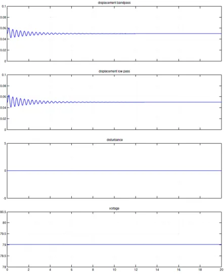
1.8.3.1 Band-Pass & Low-pass System

As explained earlier the band-pass model will be validated for 4 conditions,

When the system is inputted with DC signal optimum to maintain at midpoint, is the

equilibrium point. This voltage has been calculated in the above section. There will be

18

this case the distance between the minimum and maximum the mass can be moved is

10cm. Thus equilibrium point is 5cm. This will be seen in Figure 3.

The other condition maintained for this validation is that there is no exogenous

disturbance on the mass. This is also clearly shown in the scope represented in the

Figure 3.

It is clearly visible that the low-pass equivalent and the band-pass settles at the same set

equilibrium point proving the point the system can be sampled at just twice the

resonant frequency of the mechanical system instead that of the electrical signal which

19

20

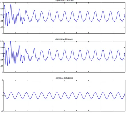
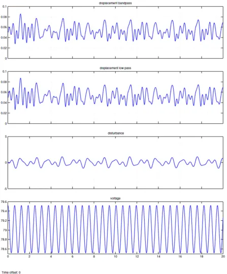
For the monochromatic disturbance as in Figure 4 is obtained when the system is

influenced by single sinusoidal disturbance. And also there is the informational signal on

to the mass i.e., the voltage signal with resonant frequency of the mass.

21

The Figure 5 is obtained for polychromatic disturbance with three disturbances of

amplitude and phase as follows, 0.5cos5t + 0.3sin11t+0.4cos8t N, at ωm. It can be

noticed that the movement of the mass is exactly the same as that of the band-pass

22

Figure 5- Polychromatic disturbance

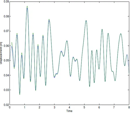
Though the displacement of the mass of band-pass system matches almost to that of

23

small difference between the displacements of the low-pass equivalent and that of the

band-pass model. This is because of the existence non-linearity in the low-pass

equivalent governing equations. This can be overcome in the two magnet model. This

will be validated and verified in the later text. But this difference is not the permanent

one, the difference voids off as the system stabilizes as the time frame increases.

24

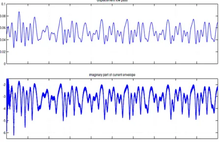
Figure 7- Displacement and imaginary current envelope comparison

Figure 7, the scope shows clearly the low-pass equivalent is that the imaginary part of

the complex current envelope is in phase of that displacement of the payload/mass.

Though there is a non-linearity difference. But for analysis of the type of vibration or

amplitude of vibration or control of vibration this result can be employed. The relation

between both the displacement and imaginary part of the current envelope could be

found out by calculating the ratio between the mean values of the both the scopes. This

will be the factor relating the two.

Figure 8 validates the setup of the limiters. The mass is not allowed to cross the

ye=10cm, as soon as it hits the values ye, the limiters comes into force setting up the

25

26

2

Two Magnet systems

2.1.1 Two- Magnet model Governing Equations

The basic governing equations are used for both types of model being discussed

henceforth. In the two magnets model there is same set of equations but for both

magnets individually. Since the mass is placed at y=0, and the electromagnets at ye/2

and -ye/2, there is equivalent displacement introduced such that influence of

displacement on the inductance of both the electromagnets could be calculated

effectively.

For left magnet, ξl5-y6ye/2, (2—1)

For right magnet, ξr5y6ye/2, (2—2)

The respective inductances of the magnets and the low pass governing equations will

have their corresponding coefficients. The electromagnetic force will be the effective

force of both the magnets on the mass. This will be shown on the hence forth results of

the simulation run of the model made using these governing equations.

The important aspect of using the two magnet model is being the advantage of using

not the predefined voltage source set to bring the mass to equilibrium. By maintaining

same current values in both the electromagnets the mass can be maintained in

equilibrium and this plays major role in control part in positioning the mass.

Now that the governing equations have been derived for both the cases, henceforth

variables will be defined and the set of values used for testing the model designed using

these governing equations.

2.1.2 Two Magnet Description

The two magnet model’s governing equations are derived similar to that of the single

27

the both the magnets on the mass. The current flow and rate of change of current are

found for both the magnets with the parameters.

Input DC signals of the electromagnets to maintain the mass at equilibrium at y=0 can

be any value with current maintained same in both the magnets. If there is change in

current and corresponding difference in voltage signal based on the potential of the

electromagnets the mass will be inclined towards that electromagnet.

Using equation for an arbitrary value of voltage current is found for one model and the

same current is used for second model to find the corresponding signal voltage.

2.1.3 Limiters for two magnet system

Limiters conditions are of similar to that of the single magnet limiters, difference being

the positioning of the electromagnets.

At y5-ye/2; y 5 0, y 5 0 & (2—3)

At y56ye/2, y 5 0, y 5 0 (2—4)

The integrators are incorporated in this too for velocity and acceleration as additional

28

29

3

Two Magnet, Band-Pass System

3.1

Model Description

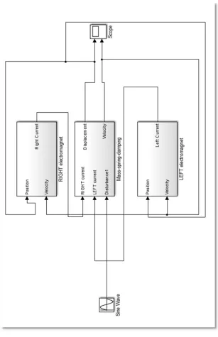
The Band-Pass system is developed by using the coupled non-linear equations afore

said. The two magnet model or the base model for all the systems is made in the

Simulink as following, the mechanical system state space decomposition constitutes a

single block which will get the influence of the current vectors from both the magnets.

In the similar way the velocity and the displacement of the mechanical system as a

result of the mutual effect of the electrical system over the mechanical influences the

electrical system.

3.2

System Equations

The system equation for one magnet is derived by splitting system in to state space

model, by splitting them into state vectors [10],

‘ 5 x’_’} (3—1)

“ 5 xq_q<_<} (3—2)

” 5  0_{9k/m 9b/m„} 1 (3—3)

•(‘) 5 –

0

—^z—Z\|˜ ™

š (3—4)

›(‘) 5 œ

0 1

9

_˜x\~˜gx]gs_Z}\|˜}„ 9

[{˜g\|˜]]

30

Ÿ(‘) 5 –_{1/[L<6 xy 6}0 ]s

} L<] š (3—6)

u 5 e (3—7)

y 5 q (3—8)

By this state- state space decomposition, the following second order final vectors are

obtained from the basic equations,

yy„ 5 9k/m 9b/m„ x0 1 yy} 6 –|^|_™0Z\|˜š 6 –_™0[š (3—9)

q_q<

<„ 5 œ

0 1

9

_˜x\~˜gx]gs_Z}\|˜}„ 9

[{˜g\|˜]] x\~˜gx]gs_Z}\|˜}žx

q<

q<} 6 œ

0

 \~˜gx]gs_Z}\|˜¡ž m

(3—10)

The above set of matrices is used in the Simulink model for the mechanical and the

electrical system correspondingly. The set of equations derived are for one side of the

magnet for the “Right Magnet”. The left magnet has similar set of matrices but the

distance of the mass from the magnet changes opposite to that of the right magnet.

3.3

Results of Band- pass system under different conditions

3.3.1 Systems displacement of mass

3.3.1.1Different voltages to both magnets and a Monochromatic disturbance

The displacement of the mechanical system which includes the influence of the current

of both the magnets and effective inductance of the system since the inductance of the

magnets is kept same value for testing purpose the influence of magnets different

currents is considered important. The effective current of the magnets on the mass and

the monochromatic disturbance 0.005 N, play role in positioning the mass since in this

particular condition the monochromatic disturbance and voltage value of the magnets

31

The maximum displacement the mass can attain is 0.05m on either side of origin. This is

explained earlier as in two cases of limits. The displacement (position) of the mass can

be effectively controlled using the voltage envelope applied compensating the

disturbance there by influencing the current. This part will explain why Low-pass model

of the electromechanical system is built and analyzed.

32

3.3.2 Systems current

Figure 11-Right Magnet Current

33

The above results are under the condition of not only a monochromatic disturbance but

34

4

Two Magnet, Low-Pass system

4.1

Systems Equations

The system equations of the mechanical system [9] is similar to that of the band-pass

system since it is already in linear form so the effective magnitude of the current in the

complex envelope form and the analytic form remains the same. Thus the mechanical

system follows similar way as that of that of the band-pass system.

The electrical system employs the low-pass equivalent system of equations that is the

complex envelope of the charge and envelope which reduces the carrier and the

information of the system and at much lower frequency there by the systems response

is effective but still maintaining the information that is linked with the mechanical

system. This also reduces the effect of non-linearity on to the mechanical systems’

displacement because the complex envelope reduces the effect of non-linearity by

eliminating the higher order variables and the effect of high frequency on them. This is

well explained in the above chapters describing the math tools used in deriving the

governing equations of the complex envelope there by deriving the low-pass system

equations.

The following equations follow the same principle as that of the band-pass system

wherein the variables are split into state space vectors and their corresponding state

space decomposition is carried out. But since the vectors of current and charge are of

complex variables the time series run results in generating complex dimension.

‘ 5 xy_y} (4—1)

“ 5 q_q<

35

” 5  0_{9k/m 9b/m„}1 (4—3)

•(‘) 5 –

0

—^z—Z\|˜ ™

š (4—4)

›(‘) 5 –_{91/[C<xL< 6 xy 6}0 ]s 1

} L<}] 9[R<6 L<y]/ xL< 6 xy 6 ]s

}L<}š (4—5)

Ÿ(‘) 5 ¢

0

 \~˜g[]gs_Z]\|˜¡£ (4—6)

‘ 5 ”‘6 •(‘) 6 d (4—7)

yy„ 5 9k/m 9b/m„ x0 1 yy} 6 – 0

—^z—Z\|˜ ™

š 6 –0[ ™š

(4—8)

“ 5 ›(‘)“6 Ÿ(‘)e (4—9)

–q< q<š 5 ¤

9jω2 1

9

_˜x\~˜gx]gs_Z}\|˜}„ 9

[{˜g\|˜]]

x\~˜gx]gs_Z}\|˜}9 jω2¥ 

q<

q<„ 6 œ

0

 \~˜gx]gs_Z}\|˜¡ž m̃

(4—10)

Similar to that in the Band-Pass system the left magnet equations are similar to that of

the right magnet varying with the distance of the mass from the position that of the

right magnet. The complex envelope of the charge and current are derived by using the

‘Hilbert Transform’, where in the pre envelope is the sum of the input signal vector and

Hilbert transform of the input signal vector in the frequency domain as shown in (1-17)

to (1-20). When converted to time domain we get real part of the analytic signal gives

the input signal vector. This is used in converting the input signal vector to complex

36

4.2

Model testing under same condition as Band-pass

4.2.1 Displacement of the system

Figure 13 – Displacement LP

The above plot displays the displacement of the mass of the Low pass equivalent system

of the electromechanical system because of a monochromatic disturbance of 0.005N

and voltage supply of 10V to right magnet and 20V to the left magnet. The below plots

are the current envelopes of the magnets with imaginary and real parts. In the future

chapters conditions used for this LP equivalent testing will be used for validation with

the perturbation model. The current envelope is since proportional to the charge

envelope, in effect the plots of the current envelope are shown and charge envelope

37

4.2.2 Current Envelope

Figure 14- Real Part of right Magnet current envelope

38

Figure 16- Real Part of left Magnet current envelope

39

5

Two Magnet, Low-Pass Perturbation System

5.1

Model description

Low-pass equivalent system is validated by linearizing with respect to electrical

subsystem variables with parameters as displacement and velocity of the non-linearly

coupled mechanical and electrical subsystems. The electrical sub-systems complex

envelope of the LP equivalent is considered and using Taylor expansion using the

Jacobian of the variables involved the subsystem is expanded and used as the electrical

subsystem.

5.2

Governing Equations of Right Magnet

5.2.1 Mechanical Subsystem

The state space variables of the subsystems is,

‘ 5 xy_y} (5—1)

“ 5 q_q<

<„ (5—2)

” 5  0_{9k/m 9b/m„} 1 (5—3)

•(‘) 5 –

0

—^z—Z\|˜ ™

š (5—4)

‘ 5 ”‘ 6 •(‘) 6 d (5—5)

yy„ 5 9k/m 9b/m„ x0 1 yy} 6 – 0

—^¦—Z\|˜ ™

š 6 –0[ ™š

(5—6)

40

5.2.2 Electrical Subsystem

The electrical subsystem state space vectors,

›(‘) 5 –_{91/[C<xL< 6 xy 6}0 ]s 1

} L<}] 9[R<6 L<y]/ xL<6 xy 6 ]s

}L<}š

(5—7)

Ÿ(‘) 5 ¢

0

 \~˜g[]gs_Z]\|˜¡£ (5—8)

“§5 F(x)x6 G(x)e< (5—9)

The above equation is the governing equation for the electrical subsystem, which is

expanded using the Taylor’s expansion and neglecting the higher order functions and

considering the steady state is also included. But since it is of negligible value when the

model is tested in Simulink the steady state component is not considered. The function

to the order of only first order is only considered [11, 12].

“©#«6 “©¬« 5 ­[›(‘#)]“©¬«6 Ÿ(‘#)®z©¬«¯ 6

­[›(¬) 9 °±²³]“©#«¯ 6

[Ÿ(¬)®z©#«] 6 6 6 6

­[›(¬) 9 °±²³]“©¬«¯ 6

[Ÿ(¬)®z©¬«]

(5—10)

The state space matrix is differentiated and variables influencing the electrical vectors

are the velocity and displacement which is termed up to “0”.

›(¬) 5 –_91/(C<[L<0₆]s 1 L<]) 9R</[L<6

]s

41 ´_µ‘µ›

‘¶¬´ 5 ¤

0 0

9 \|˜]

_˜ \~˜gs_Z\|˜¡Z 9

\|˜x]x\~˜gs_Z\|˜}b{˜]} x\~˜gs_Z\|˜}Z

¥ (5—12)

Ÿ(¬) 5 ·_1/[L<60 ]s

L<]¸ (5—13)

´_µµŸ

‘_‘¶¬´ 5 ¢

0

b\|˜]

 \~˜gs_Z\|˜¡Z£ (5—14)

“©¬«5 ¹q_q<©«

<©«º (5—15)

“©#«5 ¹q_q<©#«

<©#«º (5—16)

®z©¬« 5 ²§ (5—17)

‘©#«5  y_y©#«_©#«¡ (5—18)

›(‘#) 5 ¤

0 0

9 \|˜]

_˜ \~˜gs_Z\|˜¡Z 9

\|˜[][\~˜gs_Z\|˜]b{˜]] x\~˜gs_Z\|˜}Z

¥ (5—19)

›(‘#)“©¬« 5 ¤

0 0

9 \|˜]

_˜ \~˜gs_Z\|˜¡Z 9

\|˜x][\~˜gs_Z\|˜]b{˜]} x\~˜gs_Z\|˜}Z

¥ q_q<©«

<©«„ (5—20)

›(‘#)“©¬« 5 ¤

0 0

9 \|˜]

_˜ \~˜gs_Z\|˜¡Z 9

\|˜x]x\~˜gs_Z\|˜}b{˜]} x\~˜gs_Z\|˜}Z

¥ q_q<r©«6 jq<»©«

<r©«6 jq<»©«„ (5—21)

Ÿ(‘#) 5 ¢

0

b\|˜]

42 ­›(¬) 9 [jω2³]¯“©#«5 ¤œ

0 1

9_{_}

˜[\~˜gs_Z\|˜] 9 {˜

x\~˜gs_Z\|˜}ž 9 [jω2I]¥ 

q<r©#«6 jq<»©#«

q<r©#«6 jq<»©#«„

(5—23)

›(‘#)“©« 5

¼ ½ ½

¾ 0

9 q<r©«L<y C< L<6 y_{2 L}2 <¡

9

L<xy xL<6 y_{2 L}2 <} 9 R<y} q<r©«

xL<6 y_{2 L}2 <} ¿ À À Á 6 j ¼ ½ ½ ¾ 0

9 q<»©«L<y C< L< 6 y_{2 L}2 <¡

9

L<xy[L< 6 y_{2 L}2 <] 9 R<y} q<»©«

xL< 6 y_{2 L}2 <} ¿ À À Á (5—24)

­›(¬) 9 [jω2³]¯“©#«

5 Â

ω2q<»©#«6 q<r©#«

9 q<r©#« C<xL<6 y_{2 L}2 <}

9 q<r©#«R< xL< 6 y_{2 L}2 <}

6 q<»©#«ω2Ã

6 j Â

9ω2q<r©#«6 q<»©#«

9 q<»©#« C<xL< 6 y_{2 L}2 <}

9 q<»©#«R< xL<6 y_{2 L}2 <}

9 q<»©#«ω2Ã

5—25

[Ÿ(¬)]®z©#« 5 œ

0

43 ­›(¬) 9 [jω2³]¯“©«

5 Â

ω2q<»©«6 q<r©«

9 q<r©« C<xL<6 y_{2 L}2 <}

9 q<r©«R< xL<6 y_{2 L}2 <}

6 q<»©«ω2Ã

6 j Â

9ω2q<r©«6 q<»©«

9 q<»©« C<xL< 6 y_{2 L}2 <}

9 q<»©«R< xL<6 y_{2 L}2 <}

9 q<»©«ω2Ã

(5—27)

[Ÿ(¬)]®z©¬« 5 œ

0

x\~˜gs_Z\|˜}ž[u<r©«6 ju<»©«] (5—28)

Ÿ(‘#)®z§©¬« 5 œ

0

b\|˜]

 \~˜gs_Z\|˜¡Zž [u<r©«6 ju<»©«] (5—29)

The set of equations are derived for the right magnet are derived, the left magnet is

self- evident with only the displacement varying. The final vectors since in the complex

dimension the imaginary and real parts of the charge and current envelope are shown in

the following equations.

44 q<<5 9 q<r©«L<y

C< L<6 y_{2 L}2 <¡ 9

L<xy xL<6 y_{2 L}2 <} 9 R<y} q<r©«

xL< 6 y_{2 L}2 <}

9 q<r©#«

C<xL<6 y_{2 L}2 <}

9 q<r©#«R< xL<6 y_{2 L}2 <}

6 q<»©#«ω26 9 q<r©«

C<xL<6 y_{2 L}2 <}

9 q<r©«R< xL< 6 y_{2 L}2 <}

6 q<»©«ω26 1

xL<6 y_{2 L}2 <}

u<r©«6 1

xL<6 y_{2 L}2 <}

u<r©#«

6 9L<y  L<6 y_{2 L}2 <¡

u<r©«

(5—31)

q<= 5 9ω2q<r©#«6 q<»©#«9 ω2q<r©«6 q<»©« (5—32)

q<= 5 9 q<»©«L<y

C< L<6 y_{2 L}2 <¡ 9

L<xy xL<6 y_{2 L}2 <} 9 R<y} q<»©«

xL<6 y_{2 L}2 <}

9 q<»©#«

C<xL<6 y_{2 L}2 <}

9 q<»©#«R< xL<6 y_{2 L}2 <}

9 q<»©#«ω29 q<»©«

C<xL<6 y_{2 L}2 <}

9 q<»©«R< xL<6 y_{2 L}2 <}

9 q<»©«ω26 1

xL<6 y_{2 L}2 <}

u<»©#«6 1

xL< 6 y_{2 L}2 <}

u<»©«

6 9L<y  L<6 y_{2 L}2 <¡

u<»©«

45

5.3

Model Testing

5.3.1 Displacement of the mechanical subsystem:

Figure 18- Displacement –LP Perturb

This particular test for the perturbation analysis is carried out with the same conditions

as of the other two earlier models. Value of the disturbance is of 0.005sin 2Å/6 N. The

excitation voltage supply of the right magnet is of 10V and the left magnet is supplied

with 20V. But the model will be run for other different conditions and will be compared

46

5.3.2 Current Envelope

Figure 19- Real Part of right Magnet Current Envelope

47

Figure 21- Real part of Left Current Envelope

48

6

Validation of Low-Pass Equivalent & Low-pass Perturb

Models

6.1

Description

The LP- equivalent model and LP-perturbation model are compared in the following

sections to show the LP-Equivalent is not by neglecting the related variables and

conditions. The above methodology for the derivation of LP- equivalent of the

electromechanical systems dynamics proves the point that voltage excitation of the

electric circuit needs to be BP if it is around resonance frequency of the circuit then only

its complex envelope is needed in order to perform calculations for the output system. If

the disturbance is LP then it has some dynamic effect on the system but it will be greatly

attenuated due to the LP characteristic of the electromechanical subsystems.

Both models are combined on a single time series with same disturbance and excitation

voltages for magnets of both models are maintained the same. Three conditions in the

following pages are considered to show the comparison between the systems. The

current envelope is only shown in the plots comparison because the displacement and

velocity is coupled with the electrical system and comparison becomes self-evident for

the other variables.

6.2

Condition 1

The conditions employed for the comparison,

• External disturbance maintained zero for both systems.

• Excitation voltages of both the systems are maintained zero.

49

6.2.1 Right Magnet Real Parts

Figure 23-Zero disturbance & Zero excitation voltage

The above plot of the current envelopes of both the systems with the conditions

explained shows clearly after initial fluctuation for the system to get stablised and it

settles at the initial condition. And it is clearly evident that the LP equivalent when

compared with LP perturbation model stabilises at the same value indicating the LP

equivalents dynamics follows as such of linearized system. The above and below plots

are for the real and imaginary parts of the current envelope of the right magnet of both

50

Figure 24-Zero disturbance & Zero excitation voltage

6.3

Condition 2

The conditions employed for the comparison are:

• External disturbance maintained zero for both systems.

• Excitation voltages of both the systems are maintained 10V for both magnets.

51

Figure 25- Zero disturbance & 10V for both the magnets

The above plot shows the similarity in the behavior of both systems. With LP equivalent

varying slightly less than that of the LP linearized perturbation model. This exists

because of the non-linearity of the electromechanical systems. But the phase of the

52

6.4

Condition 3

The conditions employed for the comparison,

• External disturbance maintained 0.005N and monochromatic sine-wave for both

systems.

• Excitation voltages of both systems are maintained 10V for right magnet and 20V

for the left magnet.

• The initial conditions for steady state.

The above condition is to show complete dynamics comparison of the system reflecting

the scope. The LP disturbance is greatly attenuated due to the mechanical subsystems

LP characteristic. The difference in voltages corresponding to the difference in the

frequencies of the magnets stabilizes the systems too. This is very much followed by the

LP equivalent system. The linearized LP equivalent by perturbation analysis results

match perfectly to that of the LP equivalent system with very or negligible difference.

The dynamics of the subsystems established by the LP equivalent system using the

mathematical tools showing that the electromechanical systems information can be

established using only the complex envelope of the input signal which carries the

information and influenced by low frequency of the mechanical subsystem and

53

Figure 26- Real right current envelope at 0.005N Monochromatic disturbance and 10V

on right magnet & 20V on left magnet.

The above plots and below plots shows the comparison between the real and imaginary

parts of the right magnet’s current envelope. It is clearly visible that the phase,

magnitude of both the models is in agreement with each other. The negligible variations

54

Figure 27- Imaginary right current envelope at 0.005N Monochromatic disturbance and

55

7

Conclusion

The analysis of the dynamics of an electromechanical system considering the

non-linearity arising when the systems are coupled gives great information which could be

used for control and analysis of vibrations. The non-linearity arises because of the

mutual interaction of the magnetic force on to the mechanical system and the

interaction of the mechanical system on to the inductance of the coil.

As seen, the resonant frequency of the electrical signal is much higher than that of the

resonant frequency of the mechanical system, so the information voltage signal with

very high frequency which controls the displacement of mass other than the exogenous

disturbance is modulated. In effect the information signal is close to the resonant

frequency of the mechanical system but also has the electrical signal’s frequency as the

carrier frequency. To sample this signal the sampling rate has to be twice the highest

frequency. This increases considerably the simulation time.

Considering this the low-pass equivalent system takes the low-pass part of the

band-pass signal, that is the complex envelope, and this information signal is close to the

frequency of the mechanical system. Thus sampling rate will be just little higher than

(double) the natural frequency of the mechanical system but representing the dynamics

of the system perfectly, and reducing the simulation time considerably.

As validation and comparison between the single magnet model and the two magnet

model is made the agreement is shown clearly, however the sensitivity is higher for the

two magnet model; even slightest disturbance affects the displacement of the mass. But

with proper analysis of the current envelope on both the magnets, and the

displacement of the magnet can be stabilized faster. The measurement of the complex

56

involved, the latter could be found by the finding peak values of both and finding the

ratio.

It is also a known fact that “A charged particle cannot be held [statically] in a stable

equilibrium by electrostatic forces alone.” This calls for a feedback control for the

system.

An effective control will be of great use in the various fields where vibration has to be

analyzed or controlled. In the future works, the scope of development of MEMS is

unlimited for the time being because it’s just in the initial phase.

The validation of the LP equivalent system using the linearized LP-Perturbation model

projects the scope of developing a control system effectively to position the mass at

desired location by varying the excitation voltage compensating any external

disturbance.

The recent application which is under development of an Active Hydromagnetic Journal

Bearing [13], this employs the same principle as applying a direct electromagnetic force

on arising the shaft and levitating the shaft there by removing the surface contact as in

the case of traditional bearings. This analysis will help in the effective control design of

57

References

1. Fitzpatrick.R, Oscillations and Waves: An Introduction, CRC Press, 2013.

2. Baraniuk.R, Signals And Systems , Orange Grove Books, 2009.

3. Psarrou.D, Simulations and feedback control of non-linear coupled

electromechanical oscillators for energy conversion applications, Florida Atlantic

University, College of Engineering & Computer Science, Master Thesis- August

2011.

4. Krause.P.C., Wasiynczuk.O, Scott D.S, Analysis of electric machinery and drive

systems, Purdue University, Second Edition, IEEE Power Engineering Society,

2002.

5. Feldman.M, Hilbert Transform Applications In Mechanical Vibration - John Wiley

& Sons, Ltd, 2011 .

6. Referred Online source (http://en.wikipedia.org/wiki/Modulation)

7. Referred Online source (http://en.wikipedia.org/wiki/Nyquist%E2%80%93

Shannon _sampling_ theorem)

8. Feucht, D.L , Magnetic-Electric Analogs, Innovatia Laboratories. (n.d)

9. Everett. E, Micheal Wu, ELEC,433, Course on Architectur for wireless

communications, Rice University, - (n.d) (cmclab.rice.edu/433/notes/fitz_

bandpassnotes.pdf )

10.Xiros. N.I, Dynamical Systems, Marine engineering process Modelling, Control &

Automation, NAME6098, University Of New Orleans, 2012 Fall (Class Notes)

11.Xiros, N.I., Georgiou, I.T. Analysis of coupled electromechanical oscillators by a

band-pass, reduced complexity Volterra method., ASME-IMECE 2005, November

58

12.Xiros.N.I, Georgiou, I.T., A combined method for the investigation of coupled

bandpass-lowpass non-linear oscillators based on hilbert transform and

perturbation analysis, 2006 ASME International Mechanical Engineering Congress

& Exposition, Chicago, Illinois, USA

13.Farmakopoulos M.G, Loghis.E.K, Nikolakopoulos.P.G, Xiros.N.I, Papadopoulos.C.A,

Modelling & Control Of Electrical Actuation System Of an Active Hydromagenetic

Journal Bearing, IMEDE 2014-38346, November 14-20, 2014 Montreal

59

Appendix A

Mechanical subsystem

m = .25;

b = .25;

k = 0.1;

yem = .1;

L1 = .5;

y = u(1);

y_dot = u(2);

i_Right = u(3);

i_Left = u(4);

d = u(5);

Trig = -1;

Dy = y_dot;

if y <= (-yem/2);

Dy_dot = ( d - (k * y) - (b * y_dot) ) /m;

%dx22= (e-(x21/C)- (R*x22))/ L0 ;

if Dy_dot < 0

Dy_dot = 0;

end;

if Dy < 0

Trig = 1;

60

elseif y >= (yem/2)

Dy_dot = ( d - (k * y) - (b * y_dot) ) /m;

if Dy_dot > 0

Dy_dot = 0;

end;

%dx22= (e-(x21/C)- (R*x22))/ (L0+(L1*yem)) ;

if Dy > 0

Trig = 1;

end;

else

Dy_dot = ( (L1/4) * ( (i_Right)^2 - (i_Left)^2 ) + d - (k * y) - (b * y_dot) ) /m;

%dx22= (e-(x21/C)- (R+ ( L1*x12))* x22)/ (L0+(L1*x11))

Electrical subsystem-LP

L0 = .05; L1 = .5;

yem = .1;

R = 1;

omega_em_L = 2000;

C_L=.5e-5;

x = u(1:2);

y = u(3); y_dot = u(4);

e = u(5);

if (y <= -yem/2)

Xi_L = yem;

61

Xi_L = 0;

else

Xi_L = -y+yem/2;

end;

A = [0, 1; -1/(L0+L1*Xi_L)/C_L,

-(R-L1*y_dot)/(L0+L1*Xi_L)];

B = [0; 1/(L0+L1*Xi_L)];

Dx = (A-j*omega_em_L*eye(2))*x+B*e;

Electrical Subsystem-BP

L0 = .05; L1 = .5;

yem = .1;

R = 1;

omega_em_L = 2000;

C_L=.5e-5;

x = u(1:2);

y = u(3); y_dot = u(4);

e = u(5);

if (y <= -yem/2)

Xi_L = yem;

elseif (y >= (yem/2))

Xi_L = 0;

else

Xi_L = -y+yem/2;

62

A = [0, 1; -1/(L0+L1*Xi_L)/C_L,

-(R-L1*y_dot)/(L0+L1*Xi_L)];

B = [0; 1/(L0+L1*Xi_L)];

63

Vita

Shathiyakkumar Ganapathy Annadurai, is a Masters student of Naval Architecture &

Marine Engineering, at University of New Orleans. His career started as Marine

Engineer. And he worked with different ships which includes Oil Tankers, Pure

Car-Carriers and Bulk Car-Carriers. He holds a Bachelor’s degree in Marine Engineering and

Certificate of Competency for Marine Engineering Officers. His research interests are