DYNAMIC RATING OF TRANSMISSION LINES FOR IMPROVED WIND ENERGY INTEGRATION IN COMPLEX TERRAIN

IMPROVED WIND ENERGY INTEGRATION IN

COMPLEX

T

ERRAIN

by

Tyler Bennett Phillips

A thesis

submitted in partial fulfillment of the requirements for the degree of Master of Science in Mechanical Engineering

Boise State University

DEFENSE COMMITTEE AND FINAL READING APPROVALS

of the thesis submitted by

Tyler Bennett Phillips

Thesis Title: Dynamic Rating of Transmission Lines for Improved Wind Energy

Integration in Complex Terrain

Date of Final Oral Examination: 07 April 2014

The following individuals read and discussed the thesis submitted by student Tyler Bennett Phillips, and they evaluated his presentation and response to questions during the final oral examination. They found that the student passed the final oral examination.

Inanc Senocak, Ph.D. Chair, Supervisory Committee

Joseph C. Guarino, Ph.D. Member, Supervisory Committee

Jake P. Gentle, M.S. Member, Supervisory Committee

Foremost, I would like to express my gratitude to my advisor, Dr. Inanc Senocak, for presenting me with the opportunity to work on the research discussed in this thesis and guiding me throughout the entire process. This thesis would not have been possible without his continuous support, motivation, and immense knowledge.

I would also like toexpress my appreciationto Dr. Joe Guarinoand Jake Gentle for being members on my thesis committee and the feedback they have provided throughoutthis work. Review and feedbackfrom Phil Andersonof Idaho Powerand Kurt Myers of Idaho National Labroatory was also very appreciated. The weather dataBoiseStateUniversityhasreceivedfromthecollaborativeINLandIPCotestbed isalsoappreciated.

I also would like to thank Micah Sandusky and Rey DeLeon for their help in generating the CFD simulation, as well as everyone who has helped me throughout my studies here at Boise State University. The experience has been very beneficial to me, having been exposed to several new areas of study and learning numerous valuable skills that will most certainly help me throughout my career.

Transmission congestion is a growing concern that could limit integration of new renewable energy projects to the electricity grid. Because construction of new transmission lines is a long and expensive process, transmission service providers (TSP) are investigating dynamic line rating (DLR) methods that could potentially increase capacity of existing transmission lines. DLR is a smart-grid technology that enables rating of power lines based on real-time conductor temperature that is dependent on local weather conditions, whereas conventional practice relies on a static rating, which is based on conservative local weather assumptions to limit transmission line sag.

With today’s improved wind and weather models, communication systems, and computing hardware, a computational-based approach for DLR is a possibility. Cur-rent thesis research investigates year-long wind patterns over a large test bed area in southern Idaho, in collaboration with Idaho National Laboratory (INL) and Idaho Power Company (IPCo). To instil further confidence in the DLR approach, as proposed in the IEEE Standard 738, the ordinary differential equation (ODE) model that governs conductor temperature change in time has been first validated by coupled computational fluid dynamics (CFD) and heat transfer analysis. Both steady-state and transient thermal rating assumptions have been evaluated using field measure-ments and high order numerical methods. Under low-wind conditions, it is found that the steady-state thermal rating assumption can cause unnecessary curtailments

To better model the variation of temperature along the path of a transmission line, a large-eddy simulation (LES) of winds over the moderately complex terrain of the test bed area has been performed using clusters of graphics processing units (GPU). LES results indicate that wind speed as well as direction relative to the transmission line is a critical factor in determining the conductor temperature, which implies that numerical wind models need to provide accurate estimates of wind speed and direction in regions of complex terrain.

ABSTRACT . . . vi

LIST OF TABLES . . . xii

LIST OF FIGURES . . . xiii

LIST OF ABBREVIATIONS . . . xix

1 Introduction . . . 1

1.1 Background . . . 2

1.1.1 Renewable Energy . . . 3

1.1.2 Transmission Network . . . 3

1.1.3 Operation of Transmission Lines . . . 4

1.2 Thesis Statement . . . 6

1.3 Works Published . . . 9

2 LITERATURE REVIEW . . . 10

2.1 Smart-Grid Technology . . . 10

2.1.1 Commercial DLR Technologies . . . 11

2.2 Current DLR Technology Limitations . . . 14

2.3 Dynamic Line Rating Field Test Results . . . 15

2.4 DLR Research at Durham University . . . 16

2.5.2 Analysis of DLR Capacity Over the INL & IPCo Test Bed . . . . 20

3 Technical Background . . . 22

3.1 ACSR Transmission Conductor . . . 22

3.2 IEEE Standard 738-2006 . . . 24

3.2.1 Steady-State Heat Balance . . . 24

3.2.2 Transient Heat Balance . . . 26

Conductor Heat Capacity . . . 26

Conductor Electrical Resistance . . . 28

Solar Heating . . . 29

Convective Cooling . . . 32

Radiative Cooling . . . 33

3.3 Numerical Methods . . . 34

3.3.1 Euler Method . . . 35

3.3.2 Runge-Kutta Method . . . 36

3.4 Structure of the Atmospheric Boundary Layer . . . 39

3.4.1 ABL Mechanical Turbulence . . . 42

3.4.2 ABL Convective Turbulence . . . 43

3.4.3 ABL Surface Layer . . . 46

ABL Roughness Sublayer . . . 47

3.4.4 ABL Ekman Layer . . . 47

3.5 Numerical Wind Modeling and Prediction . . . 48

3.6 Turbulence Modeling . . . 50

3.6.1 Reynolds-averaged Navier-Stokes Equations . . . 51

3.6.3 Turbulence Closure Problem . . . 54

3.7 Standard k- Turbulent Closure Model . . . 55

4 IEEE Standard 738 Validation . . . 57

4.1 Computational Setup for the Heated Conductor Analysis . . . 57

4.2 Standard Turbulence Wall-Function . . . 59

4.3 Conjugate Heat Transfer . . . 62

4.4 IEEE Transient Temperature Calculation . . . 62

4.5 Steady-State and Transient Heating Validation . . . 66

4.6 Conclusion . . . 70

5 INL & IPCo Test Bed Analysis . . . 72

5.1 INL & IPCo DLR Motivation, Test Bed Area, and Previous DLR Analysis 72 5.2 Weather Station Selection for DLR Analysis . . . 77

5.3 DLR Capacity Results . . . 80

5.4 Conclusion . . . 81

6 DLR Using a Numerical Wind Solver Over Complex Terrain . . . . 83

6.1 Accelerated Multi-GPU Numerical Wind Solver . . . 84

6.2 Application of the Numerical Wind Solver . . . 85

6.3 Spatial Variation of Thermal Ratings Across Complex Terrain . . . 89

6.4 Conclusion . . . 97

7 DLR Utilizing a Transient Conductor Temperature Calculation . . 98

7.1 INL & IPCo Concurrent Cooling Calculation . . . 98

7.2 Transient Calculations for Conductor Temperature . . . 99

7.2.2 Season Long Test Case Comparison . . . 103

7.3 Conclusion . . . 105

8 Conclusions and Future Directions . . . 106

8.1 Conclusions . . . 106

8.2 Future Directions . . . 107

REFERENCES . . . 109

3.1 Starling 26/7 ACSR physical and electrical properties [48, 85]. . . 23 3.2 Specific heat of conductor wire materials as listed in Black and Byrd [15]. 27 3.3 Atmosphere correction coefficients [48]. . . 31 3.4 Solar azimuth constant, C, as a function of hour angle, ω, and solar

azimuth variable,χ [48]. . . 32

4.1 Normalized L2-norm of conductor temperature. Reference tempera-ture calculated with MATLABs [59] 4th _{order Runge-Kutta method}

(ode45) with a time step size of 1 second. . . 64

6.1 Calculated conductor temperature using real-time and simulated wind velocity at weather stations. . . 96

7.1 Time steady-state and transient methods indicate emergency ratings and curtailment. Temperature calculated using summer real-time weather data with a constant 849 Amp load and maximum solar heating. . . 103

2.1 Illustration of transmission span between dead-end structures when insulators are not free to rotate. Conductor temperature will vary along the length of transmission line due to different environmental conditions and tension monitoring systems will give inaccurate results with fixed insulator position [51]. . . 13 2.2 Illustration depicting freely swinging insulators that equalize the

ten-sion between load cells mounted on dead-end structures giving the average conductor temperature [51]. . . 13

3.1 Schematic of ACSR high-voltage transmission cable [44]. . . 23 3.2 Diagram of the heat balance within a conductor [45]. . . 25 3.3 Transient temperature response to a change in electrical current from a

pre-load of 800 Amps to 1,200 and 1,300 Amps. Graph adopted from [48]. 27 3.4 (a) The local truncation error over a single time step, denoted by h.

(b) Reducing the size of the time step results in a better estimation of the true solution. Illustration adopted from [18]. . . 36 3.5 Schematic of the vertical sublayer structure in the atmospheric

bound-ary layer. In this diagram, h is the boundary layer depth, z is height, and z0 is the aerodynamic roughness length [40]. . . 40

its typical evolution over land under fair weather, cloud free conditions. Heating from below sets to a convective very turbulent mixing layer during the day, while at night a less turbulent residual layer contain-ing former mixed layer air and a nocturnal stable boundary layer of sporadic turbulence (dark region). Illustration adopted from Stull [88]. . 41 3.7 Flow over a flat plate. Illustration adopted from [22]. . . 42 3.8 Flow over a two-dimensional ridge showing formation of an increased

velocity over the crest and a separation bubble when the downwind slope is steep enough [53]. . . 44 3.9 Vertical pressure gradients in warmer (right) and colder (left) air.

Planes symbolize constant pressure levels. Numbers give air pressure in hPa. Capital letters indicate high (H) and low (L) pressure at the surface (lower letters) and on constant height surfaces aloft (upper letters). Arrows indicate a thermally directed circulation. Illustration adapted from Emeis [34]. . . 45 3.10 Turbulent flow velocity fluctuations and time averaged velocity using

RANS approach. Illustration adopted from [35]. . . 51

4.1 Computational mesh generated using ICEMCFD. The conductor has been suppressed, only showing the fluid domain for visualization. The mesh quality has a minimum of 0.802 and maximum of 1, and ∼98% of the cells having a quality>0.9. . . 58

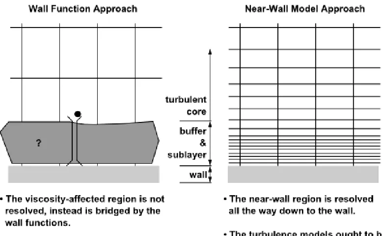
aluminum, and steel zones are shown with small wall-adjacent cell at the conductor. . . 59 4.3 Subdivisions of the near-wall region. Adopted from [10]. . . 60 4.4 The two near-wall approaches used in turbulence modeling are

de-picted. The wall function approach is shown on the left, where the flow is not resolved but bridged with the use of a wall function. On the right, the near-wall model approach is shown, here the flow is resolved using a refined mesh near the wall. Illustrations adopted from [10]. . . . 61 4.5 Transient conductor temperature solution using Euler’s method with

5, 10, and 20 minute time step size. The time step used in the IEEE digitize solution is 1 minute. . . 65 4.6 Transient conductor temperature solution using 4thorder Runge-Kutta

method with 5, 10, and 20 minute time step size. The time step used in the IEEE digitize solution is 1 minute. . . 65 4.7 ACSR conductor consists of many individual wires but is modeled as

two concentric cylinders, aluminum outer with a steel core. The outer diameter and aluminum cross-sectional area are kept constant. . . 67 4.8 Validation of IEEE Standard 738 steady state conductor temperature.

Laminar flow model was used for low wind velocity, 0.5-3 m/s, and a standard k- model with standard wall functions for velocity ranging from 2-10 m/s. Results show different cell-adjacent size near the wall. . 69 4.9 Maximum wall-adjacent y+ _{value of different wall-adjacent cell size. . . . 69}

nar CFD simulation. Here the inlet velocity is 1 m/s, giving a Reynolds number ∼1,500. . . 71

5.1 Idaho National Laboratory and Idaho Power’s dynamic line rating research test bed location in southern Idaho [41]. . . 75 5.2 Land topology and transmission line’s traversing through INL & IPCo

DLR research test bed area [41]. Weather stations are labeled and the location is indicated by a white square. . . 76 5.3 Wind velocities at all 17 weather stations from July 2012 through June

2013. Here the box represents the 75th and 25th percentile at the top and bottom, respectively, and the center line indicates the median. . . 78 5.4 Seasonal day and night wind velocity from July 2012 to June 2013 at

weather stations 7, 16, and 17. The box represents the 75th _{and 25}th

percentile at the top and bottom respectively, the center line represents the median. WS7 winter wind velocity data is deficient. . . 79 5.5 Winter wind velocity at weather stations 7, 16, and 17. Weather station

7 did not collect data over several large time spans, giving readings of 0 m/s, therefore it has been deemed deficient. . . 80 5.6 Hourly seasonal DLR at weather station 17. The horizontal line is the

static ampacity and the variable lines represent the 10th₋₉₀th _DLR

percentile from bottom to top, respectively. . . 82

6.1 Seasonal wind velocity and direction. . . 87 6.2 Wind contour over the test bed area, having a general wind flow from

the west to east direction and∼6 m/s wind velocity at 10 meters height. 88

and angle selected for validation. The selected hour long data used is between the vertical dashed lines, when direction and velocity are stable and mimic the boundary conditions imposed on the wind solver. The horizontal dashed line represents wind that is out of the west, blowing in the east direction. . . 90 6.4 Initial attempt at validation of wind flow solver over the INL & IPCo

test bed area. The mean and standard deviation of real-time hour-long (27 samples) data reading from the summer are compared with the mean wind velocity from the numerical wind solver. . . 91 6.5 Superimposed INL & IPCo test bed area and calculated conductor

temperature. The flow field incoming velocity resembles a 12.5 mph wind field out of the east. Temperature is calculated assuming 35◦C ambient temperature and 12 W/m solar heating. . . 92 6.6 Superimposed INL & IPCo test bed area and calculated conductor

temperature. The aspect is stretched in the vertical direction by a factor of 6 to better show the terrain. . . 93 6.7 Plot of transmission line temperature along its length across the test

bed area. Horizontal line represents temperature that indicates emer-gency ratings, 75◦C. . . 94 6.8 Plot showing the sensitivity of the wind direction factor, Kangle, used

in convective cooling equations. Here 0◦ is wind direction parallel to the conductor and 90◦ is perpendicular. . . 95

as described in [41–43, 45]. . . 102 7.2 Real-time conductor temperature comparison using transient and

steady-state equations. The horizontal lines represent the temperature where emergency and curtailment temperatures are reached. . . 102 7.3 Histogram of conductor temperature using real-time summer weather

data and a constant load of 849 Amps and maximum solar heating applied. . . 104 7.4 Histogram of conductor temperature above 75◦C using real-time

sum-mer weather data and a constant load of 849 Amps and maximum solar heating applied. . . 104

TSP – Transmission Service Provider

DLR– Dynamic Line Rating

SLR – Static Line Rating

CFD – Computational Fluid Dynamics

FERC – Federal Energy Regulatory Commission

EIA – Energy Information Administration

NERC – North American Electric Reliability Corporation

DOE – Department of Energy

IEEE – Institute of Electrical and Electronics Engineers

INL – Idaho National Laboratory

IPCo – Idaho Power Company

EPRI– Electric Power Research Institute

ERCOT – Electric Reliability Council of Texas

WWPTO– Wind and Water Power Technology Office

RANS – Reynold-Average Navier-Stokes

ACSR– Aluminum Conductor Steel Reinforced

ABL – Atmospheric Boundary Layer

ODE – Ordinary Differential Equation

IVP– Initial Value Problem

RK – Runge-Kutta

WAsP– Wind Analysis and Application Program

NS – Navier-Stokes

NWP – Numerical Weather Prediction

DNS – Direct Numerical Simulation

LES– Large-eddy Simulation

SGS – Subgrid-scales

WS – Weather Station

GPU – Graphics Processing Unit

BSU – Boise State University

MPI – Message Passing Interface

CUDA – Compute Unified Device Architecture

IBM – Immersed Boundary Method

CHAPTER 1

INTRODUCTION

U.S. utilities have long been under government sanctioned regulation, however they are now shifting towards a deregulated market. This has put increased pressure on transmission service providers (TSP) to increase energy transfer capacity on the existing transmission grid. Over the last several decades utility investment on trans-mission infrastructure has not kept pace with the growing generation and capacity needs [97]. Many transmission lines are already congested, and the electricity demand is predicted to grow 28% by 2040 [5]. TSPs are investigating alternative technologies such as dynamic line rating (DLR) to increase transmission capacity.

Current DLR technologies used in industry include direct line sag, line tension, and conductor temperature measurements. These technologies are expensive per unit and typically don’t take enough measurements to give an accurate assessment of the variation of conductor temperature along its length [42]. Current DLR technologies only allow average temperature calculations over large transmission spans or single point temperature measurements. Application of these systems is also not clear in regions of complex terrain.

With todays improved wind and weather modeling, communication systems, and computational capabilities, using computer simulations to determine conductor ca-pacity has become a possibility. An approach utilizing computer simulations po-tentially allows dense temperature calculations along transmission lines and has the advantage of implementation without de-energizing the lines.

However, as with any computational simulation approach, capability needs to be tested and validated before actual implementation. Therefore, one of the major goal of this thesis research is to critically investigate a DLR system using year-long weather data collected over a test bed area and computational fluid dynamics (CFD) simulations over complex terrain.

1.1

Background

1992 [91]. In 1996, the Federal Energy Regulatory Commission (FERC) issued order 888 [67] requiring all public utilities to open their transmission lines to competitors. The commission’s goal was to remove impediments to competition in the wholesale of bulk power and bring more efficient, lower cost power to consumers.

1.1.1 Renewable Energy

Due to favorable regulatory frameworks, wind energy has maintained rapid growth over the past decade. The U.S. Energy Information Administration (EIA) projects the wind energy growth to continue over the next 30 years [5]. According to the North American Electric Reliability Corporation (NERC), approximately 260,000 MW of new renewable capacity is projected over the coming ten years, of which wind will account for approximately 88% [24]. However, increasing the percentage of wind energy in the overall energy portfolio is much more complex than simply installing wind farms in windy areas. In the 20% Wind by 2030 technical report [68], the Department of Energy (DOE) has recognized the many challenges involved in increasing the amount of wind energy resources in overall electricity production. One of the largest challenges being the lack of adequate transmission infrastructure.

1.1.2 Transmission Network

need to be met along with the sitting of new transmission lines. However, public opposition is often the largest barrier of new transmission projects [93, 97]. The frequently sited poster child is the American Electric Power Wyoming-Jacksons Ferry line that took 16 years to site and construct in Virginia [24]. According to FERC, between 2000 and mid-2007, only 14 interstate high-voltage transmission lines, with a total length of 668 miles, have been built [63]. This compares with current proposals to build many thousands of miles of new long-distance transmission lines [54]. Almost a quarter of the newly constructed transmission is specifically linked to the integration of renewable generation [25].

Construction of new high-voltage transmission lines typically takes 7–10 years to plan, permit, and erect, costing upward of $1 million per mile [19, 97]. In it’s 2009 Scenario Reliability Assessment [24], NERC stated over 40,000 miles of new transmission is needed to achieve 15% generation from renewable sources. A DOE study [68] on expanding the use of wind power estimated transmission expansion to cost$60 billion by 2030. Such a level of investments may enable the industry to meet the state mandated renewable energy portfolio standards.

Ultimately, an aging transmission network is a barrier to rolling out more re-newable sources. It’s easier and faster to site rere-newable generation than the needed transmission [19,83]. Clearly, any technology developments that lead to an increase of capacity on existing transmission lines will help renewable energy project installation by relieving the need for new transmission lines.

1.1.3 Operation of Transmission Lines

transmission network [38,39]. TSPs commonly rely on SLR methods that are based on historical weather to determine a conductor’s ampacity. Ampacity is the maximum electrical current a line can carry without exceeding its sag limit or the annealing onset temperature of the conductor, whichever is lower [57, 99]. There are several environmental variables that affect the conductor temperature, such as wind speed and direction, ambient temperature, and solar radiation. As these are difficult to predict, SLR often assumes conservative assumptions, such as full sun, high ambient temperature, and low wind speeds [30, 31]. The conservative assumptions are used to prevent overheating of the conductor, resulting in low ground clearance, which might interfere with public safety. However, SLR conservative assumptions can often cause unnecessary curtailments for wind power generation [69].

DLR is a smart-grid technology that allows the rating of power lines to be based on real-time conductor temperature dependent on local weather conditions. Wind speed and its direction relative to the power line are two major factors contributing to a conductor’s temperature. Research has shown a natural synergy exists between wind power generation and conductor cooling [13].

Trial site studies have shown switching from current SLR to DLR can increase capacity by 20–70%, depending on location. Potential benefits of implementing a DLR technology includes improved system reliability and safety, reduce capital expenditures, increased efficiency of generation resources, and lower rates for utility customers.

other hand, direct temperature measurement systems only give information at a single fixed point location. The concern with these systems is that they typically don’t take enough measurements to give an assessment of the variation of temperature along a conductor’s length [42], potentially leading to an over estimation of actual ratings [81]. This may lead to unknowingly overloading transmission lines, which could potentially put the public in danger. However, a DLR system based on numerical wind prediction potentially allows for conductor temperatures to be monitored along its path at dense intervals. Equally important, this technology may not require large investments like current technologies, or have safety concerns during installation. Therefore, a computationally-based DLR technology that can safely be put into operation to expand transmission capacity is very attractive for TSPs.

1.2

Thesis Statement

The present thesis research aims to provide a foundation for a computationally-based DLR system that can estimate the conductor temperature at dense intervals along a transmission line crossing a complex terrain region in real-time. The specific objectives of the present thesis research are as follows:

• Validate the theoretical formulation presented in the Institute of Electrical and Electronics Engineering (IEEE) Standard 738-2006 using detailed CFD analysis of a heated conductor in cross-flow.

• Apply real-time weather data to the transient thermal rating approach to calcu-late conductor temperature, and compare it against the real-time steady-state thermal rating procedure presented in [41–43, 45].

• Adopt high order numerical methods in the transient thermal rating approach and assess the benefits.

• Apply a large-eddy simulation (LES) based numerical wind solver over a moder-ately complex terrain, and investigate the feasibility of a computationally based DLR system over a large area.

The present thesis is organized in the following way:

Chapter 2 summarizes the smart-grid and contributing role DLR has. Today’s commercially available DLR technologies are listed and details are given on systems commonly used in practice. This is followed by the limitations facing current DLR technologies as well as field test results. DLR research conducted at Durham Univer-sity and the joint efforts of INL & IPCo are also summarized.

comparison to numerical results using IEEE equations is completed. The model, computational mesh generation, and CFD numerical processing are described in sufficient details.

Chapter 5 summarizes the assessment on the increase in transmission line capacity DLR may potentially allow if implemented over the INL & IPCo test bed area. The test bed location and topology as well as weather measuring instrumentation is sufficiently described. Capacity results are given for each season of the year as well as the hourly evolution due to the diurnal cycle of wind across the region.

Chapter 6 is devoted to the application of a LES-based wind solver over moderately complex terrain within a hypothetical DLR system to determine conductor temper-ature along a transmission line in real-time. Wind simulation results are compared against weather station data collected over the INL & IPCo test bed area.

Chapter 7 is devoted to assess transient versus steady-state thermal rating meth-ods to calculate the real-time ampacity of transmission conductor. Both methmeth-ods make use of real-time season-long weather data, and the resulting conductor temper-ature calculations are compared to draw conclusions on their applicability.

1.3

Works Published

Works published during the course of this study:

CHAPTER 2

LITERATURE REVIEW

Transmission congestion is a growing concern that could limit integration of new renewable energy projects. The construction of new transmission lines is a long and expensive process, so TSPs are investigating DLR technologies that can increase the capacity of existing transmission lines.

This chapter presents a review of the smart-grid, as well as current DLR tech-nologies, including direct sag, line tension, and conductor temperature measurements. Additionally, the on-going research at Durham University and the joint efforts by INL & IPCo is covered in sufficient detail.

2.1

Smart-Grid Technology

reliable, and secure, while enabling better integration of new renewable technologies, such as wind and solar power [29].

One fundamental component of the smart-grid is more efficient transmission of electricity. It’s critical for TSPs to know the maximum electrical capacity that can be transmitted at any given time [47]. The idea of DLR for efficient transmission has been around for a long time, it is an economic and effective way of uprating overhead power lines [66, 87]; however, it has proven difficult in practice. Public safety is of utmost importance, concerns over the uncertainty in DLR have kept TSPs reluctant to adopt such technologies. Over the last couple of decades, there has been research, testing, pilots, demos, and actual use of DLR systems in several locations with a number of commercial methods and equipment [11, 47, 74, 99]. The smart-grid and DLR represents an unprecedented opportunity to move the energy industry into a new era of reliability, availability, and efficiency that will contribute to our economic and environmental health [3].

Several commercial DLR technologies are available, however these systems are not widely adopted in practice. Some of the DLR technologies used in industry today include direct line sag, line tension, and conductor temperature measurements. Other direct systems not as widely used include the Ampacimon [8] and Promethean RT-TLM [28]. Two available indirect systems are the ThermalRate [71] and Alstom P341 [7]. The most common DLR systems are briefly described in the order of their development, followed by the limitations these technologies face.

2.1.1 Commercial DLR Technologies

temperature, and angle of inclination. The inclination angle is used to calculate the conductor sag, which has been validated within 5 inches in 30 feet [92], and the accuracy of conductor surface temperature is within ±1 ◦C [37]. According to USi, more than 1,000 Power Donuts have been installed between 1988 and 2012.

CAT-1 is a tension monitoring system developed by the Valley Group (currently under Nexans) in 1990 [4]. Today there are over 300 tension monitoring systems installed by over 100 utilities in more than 20 countries. CAT-1 load cells are attached at dead-end structures where they monitor the mechanical tension of the conductor. When tension monitoring is implemented, insulators between dead-end structures must be freely rotating to equalize the tension along the span. If the insulators do not rotate correctly, the system can give inaccurate tension readings; this is illustrated in Figure 2.1. Freely rotating insulators will equalize the tension as illustrated in Figure 2.2. CAT-1 system measurements give the average tension between load cells. The tension is then used to calculate the conductors average temperature over the given span.

Figure 2.1: Illustration of transmission span between dead-end structures when insulators are not free to rotate. Conductor temperature will vary along the length of transmission line due to different environmental conditions and tension monitoring systems will give inaccurate results with fixed insulator position [51].

2.2

Current DLR Technology Limitations

It has been observed that conductor temperature can vary significantly along its length [33] due to variation of environmental conditions. In complex terrain, wind velocity and its direction are highly dependent on the physical surface topology, therefore conductor temperature can have large spatial variation. According to Seppa et al. [81], monitoring the line in a few discrete locations would lead to severe over or under estimations of actual line ratings. Measurements have shown spatial line temperature variation in a single span can amount to 10–20◦C [80]. A 363 meter long transmission test site at Oak Ridge National Laboratory [81], sheltered by 15 meter tall trees at one end, have shown longitudinal temperature difference between a single span, 180 meters, to be 29◦C. The same test site has shown above ground elevation change of 4.3–10.6 meters can cause temperature to vary by an average of 20◦C.

reductions of 15–20% [81].

Adding more monitoring devices would be a potential solution of the limitations facing current DLR technologies, however these systems are typically expensive, requiring many instruments to reduce error to an acceptable level [41]. Equally im-portant, implementation of direct measurement systems can prove to be challenging, as transmission lines may need to be de-energized during installation.

2.3

Dynamic Line Rating Field Test Results

The Electric Reliability Council of Texas (ERCOT) is one of eight regional re-liability councils in North America. It’s responsible for ensuring the rere-liability of the electrical network connecting 23 million Texas customers [36]. ERCOT schedules power on an electric grid with 72,500 kilometers of transmission line. In order to fully meet the interest of market participants, ERCOT has implemented an indirect DLR system, the primary purpose is to improve the economic efficiency by reflecting the change of real-time ambient weather temperature on the ratings of transmission lines. ERCOT receives temperature data from various TSPs via telemetry, on which real-time dynamic rating are determined. The increased transmission capacity using real-time ambient temperature is given in [47]; the capacity fluctuates throughout the day and lower ambient temperature during the winter provides additional conductor cooling.

ampacity between 40–80% when using real-time conditions instead of static ratings. This increase would result in significant capital cost savings in deferred transmission line projects and improved usage of existing generation resources [74].

Eco Central Networks UK has been using dynamic ratings on the 40 km Skegness-Boston 132 kV transmission line. The ratings are calculated using local weather measurements from two weather stations mounted in Skegness and Boston at the transmission line ends. The DLR uses an assumed solar heating value as well as an angle of 20◦ due to the variable wind and transmission line directions. USi Power Donut units are used to directly monitor the line temperature in three locations. Comparison of line measurements and calculated temperature values are reported to have rather good correspondence with each other. Using the DLR monitoring system on the Skegness-Boston line enables 20–50% more wind generation to be connected to the grid [11, 99].

2.4

DLR Research at Durham University

The DLR trial site in the UK is 43 square kilometers in North Wales, located just south of the coast. The terrain features a large valley containing small towns, villages, and forest. A section of transmission line approximately 20 km long, containing 5 weather stations spaced between 1 and 5 km apart is used for validation of their DLR technique.

n points, i1, i2, . . . in. The weighting factor is a function of the distance between the

points. For example, wind speed, W s, is estimated with

W sk =

P ₁

/l2 i,k

W si

P ₁

/l2 i,k

, (2.1)

where k and l are the point location and distance between the points, respectively. This method is also used for the estimation of wind direction, solar radiation, and ambient temperature. Ground roughness is taken into account using the log-law for the determination of wind speed change in height [45].

To account for the uncertainties a probability distribution for each variable is assumed, with all variables being treated statistically independent of one another. The functions involved are quite complicated and analytic derivation of the probability distribution of the line rating is not feasible. Therefore, the Monte Carlo method is employed, samples from the probability distributions of the input variables are used for deterministic calculations of the output. The results approximate the probability distribution of the line rating [45, 62].

Trial results conducted in the winter of 2008/2009 when low ambient temperatures dominate line cooling can be found in [62]. Results from the 2009 summer when wind speed and direction dominate line cooling is given in [46]. The method does not perform as well in the summer, and as a result, work to improve wind speed and direction estimation using CFD calculations is ongoing.

2.5

INL & IPCo Collaborative DLR Research

alleviate the problems current DLR technologies face. They have installed weather measurement equipment along high voltage transmission lines at 17 locations. The weather equipment collects wind speed, wind direction, ambient air temperature, and solar irradiation. The solar irradiation data was not available for the work conducted in this study. Using weather station data, they have developed a system to dynamically rate transmission lines in real-time with the use of CFD computer simulations. Development of the system is currently ongoing and some of the re-search is protected under critical infrastructure information. Additionally, they have completed an analysis of the increased transmission capacity associated with a DLR system using real-time weather station data. The DLR test site and instrumentation is fully described in Section 5.1, it’s the same test site used throughout this thesis work.

2.5.1 INL & IPCo CFD Dynamic Rating Method

The DLR system developed by INL and IPCo [41–43, 45] uses large volumes of weather and environmental measurements to perform CFD simulations. The land topography, surface roughness of the terrain, and wind conditions at the 17 weather stations are used to initialize the CFD simulations over the test area. The project team uses WindSim CFD software, which calculates the wind field with conventional steady-state 3-D RANS (Reynolds-averaged Navier-Stokes) equations and the k-

turbulence model. This technique allows wind velocity and direction to be calculated where no telemetry is available.

digital terrain model, capturing hills, valleys, ridges, and other large topographical features. A variable spaced mesh is used in the vertical direction to provide more refinement near the ground where large wind velocity gradients exist. The finished mesh incorporates ∼48 million cells in the domain, covering a land area roughly 40×37.5 kilometers.

In addition to the topographical land forms, surface roughness is also input into the model accounting for terrain effects that are smaller than the mesh: such as trees, shrubs, and buildings. The WindSim model is too computationally intensive to be executed in real-time. Therefore, the project team adopts a library approach, which uses a database of pre-simulated results. The real-time weather station readings are then used to lookup a pre-simulated result that most accurately matches the real-time weather data. The wind conditions from the selected simulation are then used to solve the IEEE steady-state thermal rating, Equation 3.3, and determine the ampacity along the entire transmission line.

A blind study using wind velocity data from a mobile meteorological tower has been done in several locations to “gage” the accuracy of wind speed modeling using this method [41,43,45]. The comparison is made between real-time field measurements and ±20% simulated wind speeds at a single model point. Although the wind speed measured by the mobile meteorological tower at times exceeds the 20% error generated from the model, measured results during the majority of the time are within this range. Wind speed is typically only outside the 20% error for 3 minute time sample. In general, modeled results at the single test point appear to be more accurate at higher wind speeds than at lower wind speeds.

conductor is typically 10–20 minutes [98]. However, during times of rapidly changing environmental or electrical current conditions, the INL & IPCo DLR method using the steady-state thermal rating equation assumption may not accurately predict the conductors true temperature, due to a conductor heat capacity.

It’s expected that an approach that calculates the transient temperature response of conductor potentially leads to more accurate assessment of conductor’s tempera-ture. Increased information about the conductor’s actual thermal condition may allow TSPs to transfer energy more efficiently and reliable. Therefore, one of the goals of this thesis is to further assess the use of steady-state assumptions when determining real-time ratings. Transient and steady-state conductor temperature calculations will be completed using real-time weather data collected over the INL & IPCo test bed area for comparison.

2.5.2 Analysis of DLR Capacity Over the INL & IPCo Test Bed

INL & IPCo conducted a study on the potential transmission capacity rating due to a hypothetical DLR implementation. Results from their study can be found in [41]. The increase of transmission capacity has been calculated for summer and winter conditions, using different average wind speed and direction. Summer results indicate capacity can potentially be increased by 35–95% and winter ratings by 98–177%.

the wind speeds. Generally wind speed doesn’t follow a normal distribution; a Weibull distribution is a better fit [58].

CHAPTER 3

TECHNICAL BACKGROUND

This chapter gives detailed background information on the IEEE Standard 738-2006 equations for calculating over-head conductor temperature. The IEEE Standard equations as well as the numerical methods used in calculation of the ODE repre-senting conductor transient temperature change in time are described in sufficient detail. Background on high-voltage aluminum conductor steel reinforced (ACSR) transmission conductor is also provided. The structures of the atmospheric boundary layer (ABL) where wind turbines and transmission conductor reside is explained and the theory of turbulence modeling with CFD is described.

3.1

ACSR Transmission Conductor

Figure 3.1: Schematic of ACSR high-voltage transmission cable [44].

Table 3.1: Starling 26/7 ACSR physical and electrical properties [48, 85].

Property Value Unit

Conductor nominal diameter 2.667 [cm] Aluminum wire diameter 4.214 [mm] Steel wire diameter 3.277 [mm] Resistance at 25◦C 8.00525 [Ω/m] Resistance at 75◦C 9.58005 [Ω/m] Aluminum specific heat 955 [J/kg·◦_C]

Steel specific heat 476 [J/kg·◦_C]

3.2

IEEE Standard 738-2006

In engineering practice, thermal ratings of overhead lines are normally calcu-lated using one of two standards: the Institute of Electrical and Electronics En-gineers (IEEE) [48] or the Conseil International des Grands Reseaux Electriques (CIGRE) [20]. Both standards follow the same concept, the balance of the heat equation. In this study, the IEEE standard 738-2006 for calculating the temperature of bare overhead conductors is used. Conductor temperature is a function of the con-ductor material properties, concon-ductor diameter, concon-ductor surface condition, ambient weather conditions, and conductor electrical current. IEEE conducted a study on various methods for calculating the heat equation to find the ampacity of transmission line conductor. The mathematical model selected in the IEEE 738 standard is based on the House and Tuttle method, as modified by ECAR [1]. The House and Tuttle formulas consider all of the essential factors without the simplifications that were made in other formulas.

3.2.1 Steady-State Heat Balance

Transmission conductor is heated from solar radiation and electrical current, and it’s cooled via convection and radiation, as illustrated in Figure 3.2. The conductor is at a steady-state thermal condition when the heat generated in the conductor equals the heat lost to the surroundings. The steady-state heat balance equation is given by

qc+qr =qs+qj, (3.1)

whereqc is the conductor convective heat loss,qr is the conductor radiated heat loss,

Figure 3.2: Diagram of the heat balance within a conductor [45].

Joule heating is the process of heat generation due to the passage of electrical current through a conductor. It’s the main source of heating in transmission line conductors, especially under high loading conditions. The Joule heating is given as

qj =I2R(Tc), (3.2)

whereI is the electrical current, R is the resistance, and Tc is the conductor

temper-ature.

I =

r

qc+qr−qs

R(Tc)

, (3.3)

and is used to calculate the steady-state ampacity using the resistance of conductor at its maximum permissible temperature. It is used in the DLR calculation procedure described in [41–43, 45].

3.2.2 Transient Heat Balance

The temperature of overhead power line conductors are constantly changing in response to changes in weather and electrical current. When a conductor at a steady-state condition undergoes weather or electrical current changes, its temperature will change in time, reaching a new steady-state temperature. A transient temperature response to a change in electrical current is shown in Figure 3.3. The rate of change the conductor experiences is calculated using the transient heat balance equation. It is expressed as

dTc

dt =

1

mCp

[qj+qs−qc−qr], (3.4)

where mCp is the total heat capacity of the conductor. The real-time conductor

temperature and its change in time, represented by this ODE, is calculated using high order numerical methods in this study.

Conductor Heat Capacity

Figure 3.3: Transient temperature response to a change in electrical current from a pre-load of 800 Amps to 1,200 and 1,300 Amps. Graph adopted from [48].

mCp =

X

miCpi, (3.5)

where mi and Cpi are the mass per unit length of ith conductor material and the

specific heat ofith_{conductor material, respectively. Values for specific heat of common}

metals used in stranded overhead conductors are listed in Black and Byrd [15]; they are given in Table 3.2.

Table 3.2: Specific heat of conductor wire materials as listed in Black and Byrd [15].

Material Specific Heat [J/kg·◦_C]

Aluminum 955

Steel 476

Conductor Electrical Resistance

The electrical resistance of bare stranded conductor varies with frequency, average current density, and temperature. The Aluminum Electrical Conductor Handbook [2] and Southwire [85] give calculated values of electrical resistance for 60 Hz AC current at 25 and 75◦C for most standard aluminum conductors.

The calculated values include the frequency-dependent skin effect for all types of stranded conductor. However, it does not include a correction for current density dependent magnetic core effects, which is significant for ACSR conductors having an odd number of aluminum layers. The resistance of single-layer ACSR conductors is shown to be increased as much as 20%, and the resistance of three-layer ACSR may be as much as 3% higher than the tabulated values [48]. Engineering judgment is needed when using these conductors.

Electrical resistance is calculated solely as a function of conductor temperature using the calculated values at 25 and 75◦C. The conductor resistance at any temper-ature, R(Tc), is found with a linear interpolation or extrapolation using

R(Tc) =

R(Thigh)−R(Tlow)

Thigh−Tlow

(Tc−Tlow) +R(Tlow), (3.6)

whereThigh is the maximum conductor temperature where the resistance is specified,

Tlow is the minimum conductor temperature where the resistance is specified,R(Thigh)

is the resistance at Thigh and R(Tlow) is the resistance at Tlow.

conductor temperature exceeds Thigh, the calculated resistance will be somewhat

low, and thus non-conservative for rating calculations. For example, based upon measurements of individual 1350 H19 aluminum strand resistance at temperature of 175 and 500◦C, give results approximately 1 and 5% higher values than calculated using Equation 3.6 with Tlow and Thigh of 25 and 75◦C, respectively. The calculated

and measured error of resistance between 25 and 75◦C is negligible [48]. Therefore, the use of Equation 3.6 is adequate for the purpose of this study.

Solar Heating

Conductor solar heating is caused by solar radiation from the sun. The magnitude of the solar heat gain depends on the geographical location, weather conditions, time of day, and time of year. The rate of solar heat gain, qs, is defined as follows

qs =αQsesin(θ)A0, (3.7)

whereα,Qse, andA0 are the solar absorptivity of the conductor, total corrected solar

radiated heat flux, and the projected area of conductor per unit length, respectively. The angle, θ, is given as

θ = arccos [cos(Hc) cos(Zc−ZL)], (3.8)

where Hc is the solar altitude of the sun, Zc is the azimuth of the sun, andZL is the

azimuth of the conductor. The solar altitude of the sun and the solar declination are defined as follows, respectively

δ = 23.4583 sin

284 +N

365 360

, (3.10)

whereLat,δ, ω, and N are the degrees of latitude, solar declination, hours from local sun noon times 15◦, and the day of the year (January 21st = 21, February 12th = 43, etc.), respectively. The total corrected solar radiated heat flux is given by

Qse=KsolarQs, (3.11)

where Ksolar and Qs are the solar altitude correction factor and the total solar and

sky radiated heat flux rate. The solar altitude correction factor is calculated by

Qs=A+BHc+CHc2+DH

3

c +EH

4

c +F H

5

c +GH

6

c, (3.12)

where Hc is the solar altitude of the sun and the variable A–G are determined using

Table 3.3.

The total heat flux elevation correction factor,Ksolar, is given as

Ksolar =A+BHe+CHe2, (3.13)

whereHe is the elevation above sea level. The variables A, B and C are given as 1.0,

1.148×10−4, and -1.108×10−8, respectively. The solar azimuth,Zc, is given as

Zc=C+ arctan(χ), (3.14)

Table 3.3: Atmosphere correction coefficients [48].

Clear Atmosphere Value

A -42.2391

B 63.8044

C -1.9220

D 3.46921×10−2

E -3.61118×10−4

F 1.94318×10−6

G -4.07608×10−8

Industrial Atmosphere Value

A 53.1821

B 14.2110

C 6.6138×10−1

D -3.1658×10−2

E 5.4654×10−4

F -4.3446×10−6

G 1.3236×10−8

χ= sin(ω)

sin(Lat) cos(ω)−cos(Lat) tan(δ). (3.15) The solar azimuth constant,C, is a function of the hour angle and the solar azimuth variable; it is determined using Table 3.4.

Table 3.4: Solar azimuth constant, C, as a function of hour angle,ω, and solar azimuth variable, χ [48].

Hour Angle χ ≥0 χ <0

−180 ≤ω <0 0 180

0≤ω ≤180 180 360

Convective Cooling

The convective heat loss is defined dependent on wind velocity. For zero, low, and high wind velocities convective heat loss, qc, is defined as follows: for zero wind

velocity or natural convection

qcn = 0.0205ρ

0.5

f D

0.75_(T

c−Ta)1.25, (3.16)

for low wind velocity

qc1 =

"

1.01 + 0.0372

DρfVw

µf

0.52#

kfKangle(Tc−Ta), (3.17)

and for high wind velocity

qc2 =

"

0.0119

DρfVw

µf

0.6

kfKangle(Tc−Ta)

#

. (3.18)

Here ρf, µf, andkf are the air density, dynamic viscosity, and thermal conductivity

of air, respectively. The convective cooling is determined by using the largest of the three convection equations. To take into account the wind direction, the convective heat loss rate is multiplied by the wind direction factor,Kangle, which is given by

where φ is the angle between the wind direction and the conductor axis. For both forced and natural convection, air density, air viscosity, and coefficient of thermal con-ductivity of air are calculated using the film temperature,Tf ilm. The film temperature

is given as

Tf ilm =

Tc+Ta

2 . (3.20)

Dynamic viscosity of air, air density, and thermal conductivity of air are defined as follows, respectively

µf =

1.458×10−6_(T

f ilm+ 273)1.5

Tf ilm+ 383.4

, (3.21)

ρf =

1.293−1.525×10−4_H

e+ 6.379×10−9He2

1 + 0.00367·Tf ilm

, (3.22)

kf = 2.424×10−2+ 7.477×10−5Tf ilm−4.407×10−9Tf ilm2 . (3.23)

Radiative Cooling

Thermal radiation is the emission of electromagnetic waves generated by the thermal motion of charged particles in matter [49]. The radiative heat loss of a conductor is given as

qr= 0.0178Dε

"

Tc+ 273

100

4

−

Ta+ 273

100

4#

, (3.24)

whereTais the ambient temperature, Dis the conductor diameter,εis the conductor

of conductor, the absorptivity and emissivity constants range between 0.23–0.91 [48]. They are assumed to be 0.5 in this thesis.

3.3

Numerical Methods

The conductor temperature rate of change, given in Equation 3.4, is a differen-tial equation. Differendifferen-tial equations are composed of an unknown function and its derivative(s). More specifically, it’s a first order ODE. The conductor temperature is continually changing in response to electrical current and weather changes. ODEs of this form are termed initial value problems (IVPs); the general form is expressed as

dy

dx =f(t, y), (3.25)

over a time interval

a≤t ≤b,

subject to an initial condition

y(a) = yo. (3.26)

The general expression is solved conveniently using a time-marching method as follows

yi+1 =yi+φh. (3.27)

Here the slope estimate, φ, is used to extrapolate from an old value, yi, to a new

value, yi+1, over a time step size, h.

approximate values of y. Truncation errors are composed of two parts: the single step or local truncation error, and a propagated truncation error, which occurs on successive steps. The sum of truncation error is the total or global truncation error. Round-off error is caused by the limited numbers of significant digits a computer can retain.

Insight into the magnitude and properties of the truncation error can be gained by deriving numerical methods directly from the Taylor series expansion. The Taylor series expansion about a starting value (ti, yi) is given as

yi+1 =yi+f(ti, yi)h+

f0(ti, yi)

2! h

2_{+· · ·+} fn −1_(t

i, yi)

n! h

n_+O(hn+1_{), (3.28)}

wherenis the order of the solution method andO(hn+1) is the local truncation error, it is proportional to the step size raised to the (n+ 1) power. The truncation error occurs because the true solution is approximated by using a finite number of terms in the Taylor series.

3.3.1 Euler Method

The simplest method for solving an ODE is Euler’s method. It is a first order method, where the slope at the beginning of the time interval is taken as an approx-imation of the slope over the entire interval. Starting with the general form of an initial value problem, the first derivative provides a direct estimate of the slope, φ, at the initial time, ti, given as

(a) (b)

Figure 3.4: (a) The local truncation error over a single time step, denoted by h. (b) Reducing the size of the time step results in a better estimation of the true solution. Illustration adopted from [18].

Here f(ti, yi) is the differential equation evaluated at ti and yi, the initial value.

Substituting this into Equation 3.27, gives the form

yi+1 =yi+f(ti, yi)h, (3.30)

and is known as a forward Euler method.

Figure 3.4 explains the Euler method graphically. Here (a) shows the local truncation error over a single time step, while the global truncation error can be seen over multiple steps in (b). It can be seen that reducing the step size reduces the truncation error, resulting in a better estimation of the true solution.

3.3.2 Runge-Kutta Method

(RK) methods achieve higher order accuracy without requiring the calculation of higher derivatives. A full derivation of the RK method can be found in [18]; the general form is given as

yi+1 =yi+φ(ti, yi, h)h, (3.31)

whereφ(ti, yi, h) is called the increment function, which is a representative slope over

the interval h. The increment function’s general form is

φ =a1k1+a2k2+· · ·+ankn, (3.32)

where the a’s are constants and the k’s are defined as

k1 =f(ti, yi), (3.33)

k2 =f(ti+p1h, q11k1h), (3.34)

k3 =f(ti+p2h, yi+q21k1h+q22k2h), (3.35)

· · ·

kn =f(xi+pn−1h, yi+qn−1,1k1h+qn−1,2k2h+· · ·+qn−1,n−1kn−1h). (3.36)

Values for the a’s, p’s and q’s are evaluated by setting the increment function equal to terms in the Taylor series expansion. The k’s are reoccurring, k1 appears in the

order Taylor series expansion methods, this recurrence makes RK methods especially efficient for computer calculations.

Various types of RK methods can be devised by employing a different number of terms in the increment function, specified by n. For a second and fourth order RK, the increment function will have two and four terms, respectively. RK methods have an infinite number of variations. There is one less equation than unknowns when solving the a’s, p’s and q’s, an assumption of a value must be selected for one of the unknowns. Three of the most popular second order RK methods, the midpoint, Heun, and Ralston’s, are given respectively,

yi+1 =yi+k2h, (3.37)

yi+1 =yi+

1 2k1 +

1 2k2

h, (3.38)

yi+1 =yi+

1 3k1 +

2 3k2

h. (3.39)

The most commonly used fourth order RK method is given as

yi+1 =yi +

1

6(k1+ 2k2+ 2k3+k4)h. (3.40) Here the k’s represent a slope given as

k2 =f

ti+

1

2h, yi+ 1 2k1h

, (3.42)

k3 =f

ti+

1

2h, yi+ 1 2k2h

, (3.43)

k4 =f(ti+h, yi+k3h). (3.44)

The multiple estimates of the slope are developed in order to come up with an improved average slope over the time step interval. In this thesis work, a 4th order Runge-Kutta method is used to solve the IEEE ODE that governs the transient temperature change of conductor. This is done using MATLABs built-in ode45 solver [59].

3.4

Structure of the Atmospheric Boundary Layer

The troposphere is the lowest layer of the earth’s atmosphere. Its height is roughly 7 and 20 kilometers at the poles and equator, respectively. It can be divided in two parts, the atmospheric boundary layer (ABL) that extends 1–2 kilometers up from the surface occupying 10–20% of the troposphere and the free atmosphere [96]. The ABL is characterized by its behavior being directly influenced by the Earth’s surface. It is the region most directly influenced by the exchange of momentum, heat, and water vapor [53]. The most dramatic temperature changes occur within the ABL.

ABL Vertical Structure

Figure 3.5: Schematic of the vertical sublayer structure in the atmospheric boundary layer. In this diagram, h is the boundary layer depth, z is height, and z0 is the aerodynamic roughness length [40].

is directly influenced by the presence of the Earth’s surface, and responds to surface forcing with a time scale of about an hour or less.” The ABL is vertically divided into two sublayers, the sublayer height depends upon the rate at which shearing stress vary. The lower layer is the inner Prandtl or surface layer and the outer layer is the Ekman or transition layer. At the bottom of the surface layer, a roughness sublayer is present that is influenced by physical characteristics of the surface. Figure 3.5 illustrates the vertical structure within the ABL.

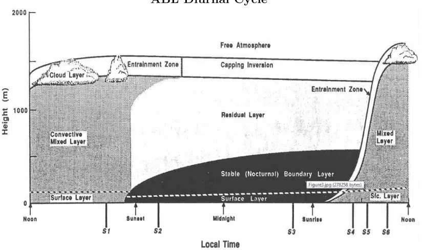
ABL Diurnal Cycle

Figure 3.6: Vertical cross-section of the atmospheric boundary layer structure and its typical evolution over land under fair weather, cloud free conditions. Heating from below sets to a convective very turbulent mixing layer during the day, while at night a less turbulent residual layer containing former mixed layer air and a nocturnal stable boundary layer of sporadic turbulence (dark region). Illustration adopted from Stull [88].

stresses are regarded as negligible and it responds very slowly to surface events. There is a buffer region between the free atmosphere and the boundary layer, termed the entrainment zone. Entrainment occurs when air from a non-turbulent free atmosphere is drawn into an adjacent turbulent region. Figure 3.6 shows how the sublayers of the ABL evolve throughout a typical cloud free diurnal (daily) cycle.

Figure 3.7: Flow over a flat plate. Illustration adopted from [22].

chaotic motions. Turbulence in the ABL differs from that studied in wind tunnels. Unlike wind tunnels, turbulence associated with thermal or convective mixing coexists with mechanical turbulence [40].

3.4.1 ABL Mechanical Turbulence

Mechanical turbulence results from wind shear due to viscous effects of the fluid. The magnitude of mechanical turbulence depends on the wind speed, roughness of the terrain, and stability of the air. Flow over a smooth flat plate is the most common and basic way to study mechanical turbulence. The boundary layer forms downstream from the leading edge of the plate, extending up where the velocity is 99% of the free stream velocity [64]. The no-slip surface condition and viscous forces generate shear stress turbulence. Initially the flow over a flat plate is laminar, but after covering some distance, fully turbulent flow is developed, illustrated in Figure 3.7.

by the surface roughness and the physical terrain. Rough flow occurs when the shear stress is dominated by the drag of the roughness elements, and in smooth flow shear stress is dominated by viscosity [73]. A better model for atmospheric flow is a rough wall boundary layer, where both smooth wall shear and fixed objects generate mechanical turbulence.

Turbulent wake structures occur when wind flows over or around large terrain and obstructions. More and more wind turbines are being built away from flat regions in complex terrain. Elevated positions like hill tops are favorable sites due to the increased wind velocity. In complex terrain, wake turbulence may occur behind structures and rapid changing terrain. Flow over a two-dimensional ridge is an example of wake turbulence and is shown in Figure 3.8. There is an elevated wind velocity over the crest of the ridge, separation on the downwind slope where flow reverses direction, and a highly turbulent wake region follows.

The CFD simulations completed in this thesis are in a region of moderately complex terrain. Because of the turbulent effects that occur in these regions, it’s necessary to use a computational mesh and turbulent model that can adequately resolve the turbulent flow characteristics that occur.

3.4.2 ABL Convective Turbulence

Figure 3.8: Flow over a two-dimensional ridge showing formation of an increased velocity over the crest and a separation bubble when the downwind slope is steep enough [53].

to buoyancy forces. Two principal types of thermal stability can be distinguished. If heating from below dominates, there is a convective or unstable ABL with high turbulence. If cooled from below, a stable boundary layer with low turbulence will exist.

Earth’s surface is heated differently according to latitude, season, and surface properties. The uneven surface heating heats the layer of air nearest the ground at different rates, causing horizontal heat gradients. The vertical distance between two given levels of constant pressure depends on air temperature [34]. Warm air is less dense and has a larger vertical distance between two given pressure surfaces than colder air. Mathematically this is described by the hydrostatic equation, given as

∂p

Figure 3.9: Vertical pressure gradients in warmer (right) and colder (left) air. Planes symbolize constant pressure levels. Numbers give air pressure in hPa. Capital letters indicate high (H) and low (L) pressure at the surface (lower letters) and on constant height surfaces aloft (upper letters). Arrows indicate a thermally directed circulation. Illustration adapted from Emeis [34].

where p is air pressure,z is the vertical coordinate, g is gravity, and ρ is air density. Assuming a constant surface pressure, this will result in horizontal pressure gradients. These pressure gradients produce compensating winds, blowing from higher pressure towards lower pressure to remove them. In reality, there isn’t a constant surface pressure and a small pressure sink occurs in warmer regions; this is illustrated in Figure 3.9.

There are local wind systems that do not emerge from large global scale temper-ature differences, but from local tempertemper-ature differences. Local wind systems, much like global systems, often exhibit a large regularity of daily and seasonal wind and weather cycles [26]. This regularity is attributed to the local terrain and surface properties.

3.4.3 ABL Surface Layer

The surface layer represents the bottom 10% of the ABL and is of particular importance in this study because it’s where transmission lines and wind turbines reside. During the day, high convective turbulence can push the surface layer to heights of ∼200 meters. At night, when convective turbulence dies, the top of the surface layer drops to ∼100 meters [34, 88] and under strong stable conditions it can be even lower. The surface layer is defined meteorologically as the layer where the turbulent vertical fluxes of momentum, heat and moisture deviate less than 10% from their surface values, and the influence of the Coriolis force is negligible [34]. The most important features of the surface layer is the highly turbulent flow where viscous forces dominate and the wind speed increases strongly with height. A logarithmic wind profile or power-law are often used to extrapolate the wind velocity, they are only valid in the surface layer. The logarithmic wind profile is given as

u(z) = u∗

k

ln

z

z0

+ψ(z, z0, L)

, (3.46)

whereu is the horizontal wind speed,u∗ is the friction velocity, k is the von Karman

stability term is equal to zero and drops out. The logarithmic wind profile is derived from physical and dimensional arguments. However, the power-law can be convenient to use; it is found empirically and is given as

u(z) =u(zr)

z

zr

α

, (3.47)

where zr is a reference height and α is the power law exponent. The power law

exponent depends on the surface roughness and the thermal stability.

ABL Roughness Sublayer

At the bottom of the surface layer, a roughness sublayer exists, referred to as the micro-layer. The micro-layer can be considered as the region influenced directly by the elements; it’s where molecular diffusion is an important process by which heat and mass are exchanged between the surface and the air [40]. The top of the micro-layer layer is the roughness length (zo), the height above the ground where wind speed is

theoretically zero [40, 88]. In reality, wind in the micro-layer is not zero, it no longer follows the mathematical logarithm velocity profile. The roughness layer depth is affected by surface topography and physical features. It’s not a physical length; it’s a length scale that represents the roughness of the surface. Estimates of the roughness length are usually determined from observations of the wind profile, preferably in neutral conditions [40].

3.4.4 ABL Ekman Layer

turning of the wind direction with height. It’s the layer where the flow is a result of the pressure gradient, Coriolis, and turbulent drag forces. In the outer region, the flow shows little dependence on the physical terrain of the surface.

3.5

Numerical Wind Modeling and Prediction

Linear wind flow models such as WAsP [32] (Wind Analysis and Application Program) are widely used to predict the spatial variation of the average wind speed, directional frequency, wind shear, and other boundary layer characteristics. Linear models gained wide use in the 1980s due to the simple turbulence and surface rough-ness models requiring limited computing resources. They run fast while performing reasonably well where the wind is not significantly affected by nonlinear phenomena. The WAsP model is best suited for simple geometries and is known to poorly predict flow separation and recirculation [17]. Its strength is in simple regions. Transmission lines and wind farms are now being placed in complex terrain where linear models have been pushed past their limitations [70].

Computational fluid dynamic (CFD) models solve the complex Navier-Stokes (NS) equations that govern the physical phenomena of fluid flow as well as heat transfer. They are derived from Newton’s second law with the assumption that fluid stress is the sum of a diffusing viscous term plus a pressure term. Solutions to the NS equations give a velocity or flow field, which describes the velocity of the fluid at a given point in space and time. The general form of the NS equations is given as

ρ

∂v

∂t +v· ∇v

=−∇p+∇ ·_T+f, (3.48)