The Thirty-Third AAAI Conference on Artificial Intelligence (AAAI-19)
Deep Convolutional Sum-Product Networks
Cory J. Butz
[email protected] University of ReginaCanada
Jhonatan S. Oliveira
[email protected]University of Regina Canada
Andr´e E. dos Santos
[email protected]University of Regina Canada
Andr´e L. Teixeira
[email protected] University of ReginaCanada
Abstract
We give conditions under whichconvolutional neural net-works (CNNs) define valid sum-product networks (SPNs). One subclass, calledconvolutional SPNs (CSPNs), can be implemented using tensors, but also can suffer from being too shallow. Fortunately, tensors can be augmented while maintaining valid SPNs. This yields a larger subclass of CNNs, which we calldeep convolutionalSPNs (DCSPNs), where the convolutional and sum-pooling layers form rich di-rected acyclic graph structures. One salient feature of DC-SPNs is that they are a rigorous probabilistic model. As such, they can exploit multiple kinds of probabilistic reason-ing, includingmarginalinference andmost probable expla-nation(MPE) inference. This allows an alternative method for learning DCSPNs using vectorized differentiable MPE, which plays a similar role to the generator ingenerative ad-versarial networks(GANs). Image sampling is yet another application demonstrating the robustness of DCSPNs. Our preliminary results on image sampling are encouraging, since the DCSPN sampled images exhibit variability. Experiments on image completion show that DCSPNs significantly outper-form competing methods by achieving several state-of-the-art
mean squared error(MSE) scores in both left-completion and bottom-completion in benchmark datasets.
Introduction
Generative models are of current interest in the deep learning community, includinggenerative adversarial net-works(GANs) (Goodfellow et al. 2014), variational auto-encoders (Kingma and Welling 2014), neural autoregres-sive distribution estimators (Larochelle and Murray 2011), pixel recurrent neural networks (Oord, Kalchbrenner, and Kavukcuoglu 2016), and convolutional arithmetic circuits (Sharir et al. 2018).Convolutional neural networks(CNNs) (Goodfellow, Bengio, and Courville 2016) can be used in GANs. Sum-product networks (SPNs) (Poon and Domin-gos 2011) are a generative model that have received limited attention from the deep learning community (Peharz et al. 2018). An SPN is adirected acyclic graph (DAG), where leaf nodes are tractable distributions and each internal node is either a sum or product operation. AvalidSPN defines a joint probability distribution and allows for efficient infer-ence (Poon and Domingos 2011).
Copyright c2019, Association for the Advancement of Artificial Intelligence (www.aaai.org). All rights reserved.
Conditions are given as to when subclasses of CNNs de-fine valid SPNs, including convolutional layer filters of cer-tain sizes and non-overlapping windows in sum-pooling lay-ers. Satisfaction of these conditions yields a subclass of CNNs, calledconvolutionalSPNs (CSPNs). CSPNs permit a vectorized representation allowing for exploitation of tensor libraries such as Tensorflow, but they also can suffer from being too shallow, and it is known that deep SPNs are more expressive than shallow SPNs (Delalleau and Bengio 2011). We introducedeep convolutional sum-product networks (DCSPNs). DCSPNs permit the convolutional and sum-pooling layers to form rich DAG structures by augmenting layer tensors under conditions that maintain decomposabil-ityandcompleteness. As a decomposable and complete SPN is a valid SPN, our main result is that DCSPNs are a larger subclass of CNNs that define valid SPNs. DCSPNs are a rig-orous probabilistic model. As such, they can exploit prob-abilistic reasoning, including marginal inference andmost probable explanation (MPE) inference. This allows an al-ternative method for learning DCSPNs using vectorized dif-ferentiable MPE. We show how to vectorize MPE using a mask algorithm and how it plays a role similar to the GANs generator. Image sampling is yet another application demon-strating the robustness of DCSPNs. This involves a minor modification to the mask algorithm. Our preliminary results on image sampling are promising, since the DCSPN sam-pled images exhibit variability. Experimental results on left-and bottom-completion like those in Table 1 show DCSPNs achieve state-of-the-art by building deeper structures using both vertical and horizontal sum-pooling windows, which leverage local structure in the image data in both direc-tions. Applying a simple low pass filter as a post-processing smoothing operation lowers themean squared error(MSE) score from455to401for left-completion in Olivetti.
Table 1: Mean squared error (MSE) scores in Olivetti Face.
left bottom P&D (Poon and Domingos 2011) 942 918 ICNN (Amos, Xu, and Kolter 2017) 833 -D&V (Dennis and Ventura 2012) 779 782 DCGAN (Yeh et al. 2017) 935 707
Sum-Product Networks
We denote random variables by uppercase letters, such as X and Y, possibly with subscripts, and their values by corre-sponding lowercase letters x and y. Sets of random variables are denoted by boldfaced uppercase letters and their com-bined values by corresponding boldfaced lowercase letters.
A sum-product network (SPN) (Poon and Domingos 2011) over variablesXcan be defined as adirected acyclic graph(DAG) containing three types of nodes: leaf distribu-tions, sums, and products. Leaves are tractable distribution functions over Y ⊆ X. Sum nodes S compute weighted sumsS = P
N∈Ch(S)wS,NN, whereCh(S)are the
chil-dren ofSandwS,N are weights that are assumed to be
non-negative and normalized (Peharz et al. 2015). Product nodes
P computeP =Q
N∈Ch(P)N. The value of an SPN,
de-notedS(x), is the value of its root.
Thescopeof a sum or product nodeN is recursively de-fined assc(N) = S
C∈Ch(N)sc(C), while the scope of a
leaf distribution is the set of variables over which the dis-tribution is defined. A validSPN defines a joint probabil-ity distribution and allows for efficient inference (Poon and Domingos 2011). The following two structural constraints on the DAG guarantee validity. An SPN iscompleteif, for every sum node, its children have the same scope. An SPN isdecomposableif, for every product node, the scopes of its children are pairwise disjoint.
Nodes of an SPN can be organized as layers for a vector-ized implementation. The discussion here draws from (Ver-gari, Di Mauro, and Esposito 2016). The SPNinput layeris formed by the leaf distribution nodes. LetL(x)∈IRsbe the output of a generic layer withsnodes and inputx. The value of asum layerwith an inputxfromrinput nodes is
L(x) =log(w×x), (1)
wherew ∈ IRs×r is a matrix of weights defining sparse connections:
wij=
wij if edge(i, j)exists
0 otherwise
andx∈[0,1]rrepresents the input probability values.
Sim-ilarly, the value of aproduct layerwith inputxis
L(x) =exp(p×x), (2)
wherep∈ {0,1}s×ris a matrix of sparse connections:
pij=
1
if edge(i, j)exists 0 otherwise
andx∈[0,1]rrepresents the input probability values in log-space. In this formulation, the exponential and logarithmic functions act as nonlinearities.
In our paper, we relate SPNs with convolutional neu-ral networks (CNNs) (Goodfellow, Bengio, and Courville 2016). In general, CNNs are formed by convolutional and pooling layers. Aconvolutional layercan be constructed by applying a convolutional operation with afilteron a previ-ous layer output. Apooling layercan be built by applying a max or average operation over some elements of the previ-ous layer with respect to a slidingwindow. A sum-pooling layer can be easily obtained from an average-pooling layer.
Convolutional SPNs
We study when subclasses of CNNs define valid SPNs. First, note that a vectorized SPN can represent a CNN. SPN sum layers correspond to CNN convolutional layers. Here, sum layer weights are convolutional filters and the sum layer value computes the convolution operation. Sim-ilarly, SPN product layers correspond to CNN sum-pooling layers. The sum-pooling window computes the product layer value in log-space.
Example 1 Figure 1 illustrates an SPN with 3 layers being represented by a CNN with 3 layers, where colours represent node scopes. The input layer is the same for both, while the sum and product layers in the SPN are convolutional and sum-pooling layers in the CNN, respectively.
Conversely, we show how a CNN can represent a vector-ized SPN in log-space. Representational, convolutional, and sum-pooling layers in CNNs can represent the input, sum, and product layers in SPNs, respectively.
Arepresentational layer(Sharir et al. 2018) is formed by applyingnrepresentation functionsf1, . . . , fn : IRs→IR
over s-dimensional local patches of the dataset. We apply the logarithmic function in representational layers so as to correspond to SPN input layers in log-space. For instance,
nGaussian distributions can be used as representation func-tions to map patches of dataset instances tonvalues in the representational layer.
The value of aconvolutional layerwith inputxis com-puted element-wise depending on filterw’s size with depth
cbeing eitherm-by-n(top) or height-by-width (bottom):
Lij(x) =
( Pm−1
q=0 Pn−1
l=0 log(wql) +x(i+q)(j+l) Pc−1
k=0log(wijk) +xijk.
(3)
Convolutional layers in (3) relate to sum layers in (1). The value of a sum-pooling layer with sliding window sizem-by-nand inputxis computed element-wise as:
Lij(x) = m−1
X
q=0
n−1 X
l=0
x(i+q)(j+l). (4)
Figure 2: A CSPN represents a valid SPN and is vectorized, but also can suffer from being shallow.
Sum-pooling layers in (4) relate to product layers in (2). We now define a subclass of CNNs that represent SPNs by restricting convolutional and sum-pooling layers.
Definition 1 Aconvolutional SPN(CSPN) is a CNN formed under the following two restrictions: (i) convolutional layer filters must have height and width of 1-by-1 or h-by-w, wherehandware the height and width of the convolutional layer, respectively; (ii) in sum-pooling layers, the horizontal and vertical stride of the sliding window must be at least the width and the height of the window itself, respectively.
Example 2 Consider the CSPN illustrated in Figure 2, where colours represent node scopes. The dataset is mapped to a 4-by-4 representational layer using 2 representation functions. Next, a convolutional layer is formed with 6 filters of size 4-by-4. A 2-by-2 sum-pooling layer is then built with a 2-by-2 sliding window. Finally, the root node is a 1-by-1 convolutional layer obtained using one 2-by-2 filter.
Next, we show that CSPNs represent valid SPNs.
Theorem 1 LetCbe a CSPN formed with respect to a CNN
C0in Definition 1. Then,Cis avalidSPN.
Proof 1 To be valid,Cmust be bothcompleteand decom-posable. The restriction on each convolutional layer filter in C0 to be 1-by-1 or h-by-w ensures that the sum in the
convolution operation in (3) occurs over elements of the same scope. Thus,Cis complete. The restriction on the sum-pooling layers with the horizontal and vertical stride of the sliding window being at least the size of the window itself guarantees that the multiplication (summation, in log-space) in the pooling operation in (4) occurs over elements with dis-joint scopes in the current and subsequent layers. Therefore,
Cis decomposable. By definition,Cis a valid SPN.
CSPNs can struggle with depth, since the sum-pooling window size quickly reduces the size of the layers. For ex-ample, as depicted by the CSPN in Figure 2, the 4-by-4 rep-resentational layer reduced to the 1-by-1 root layer after two convolutions and one sum-pooling operation. As deep SPNs are more expressive than shallow SPNs (Delalleau and Ben-gio 2011), we now turn our attention to introducing deep CSPNs.
We build deep CSPNs by considering two related issues. First, we seek a DAG structure rather than a chain structure. Second, since each node is implemented as a tensor, each combination of tensors must be done such that a valid SPN is maintained. The next section formalizes these ideas.
Deep Convolutional SPNs
In this section, we introduce a tractable generative model, calleddeep convolutional SPNs(DCSPNs).
We denote by T a tensor of rank (order) n and dimen-sionmin each mode. That is,T is a multi-dimensional ar-ray, specified by a shape withnindexes[d1, . . . , dn], each
ranging in[m]≡ {1, . . . , m}. Without loss of generality, a layer is represented as a rank 4 tensor with shape[b, h, w, c], wherebis the batch (number of instances) being considered, andh,w, andcare the height, width, and channel (depth), respectively. Tensor elements are SPN nodes. In a sum layer tensor, elements are sum nodes, while in a product layer, tensor elements are product nodes.
LetT1andT2be two tensors with the same height and the
same width. Thechannel augmentationofT1andT2is the tensor with the same height and the same width formed by concatenatingT1andT2with respect to the channel axis.
Example 3 LetT1andT2be the two tensors in Figure 3 (a) (left, right), respectively. Then, the channel augmentation of
T1andT2is the tensor depicted in Figure 3 (b).
Let T1 and T2 be two tensors with the same depth and height. Thewidth augmentation ofT1 andT2is the tensor with the same depth and the same height formed by concate-natingT1andT2with respect to the width axis. Theheight augmentationis defined similarly.
Example 4 LetT1andT2be the two tensors in Figure 3 (c) (left, right), respectively. Then, the width augmentation ofT1
andT2is the tensor depicted in Figure 3 (d).
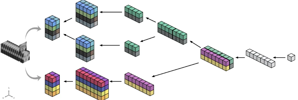
Definition 2 A deep convolutional sum-product network (DCSPN)DovernvariablesX1, . . . , Xnis a rooted DAG
whose leaves are representational layers and whose internal nodes are convolutional and sum-pooling layers. A convolu-tional layer with more than one child is formed by recur-sively applying channel augmentation on all its children. A
(a) (b) (c) (d)
Figure 4: A DCSPN, depicting a rich DAG structure of convolutional and sum-pooling layers, while still being a valid SPN.
sum-pooling layer with more than one child is formed by re-cursively applying either height or width augmentation on all its children.
Example 5 Consider the DCSPN in Figure 4. The dataset is mapped to 2 representational layers, each using 2 represen-tation functions. In the upper branches, after a convolutional and a sum-pooling layer, a channel augmentation is used to form a convolutional layer. In the lower branch, after a convolutional and sum-pooling layer, a width augmentation is used to form a sum-pooling layer. Lastly, a sum-pooling layer is followed by the root convolutional layer.
By construction, DCSPNs represent SPNs. We now pro-vide structural conditions under which DCSPNs represent valid SPNs.
Lemma 1 Consider a DCSPNDwhere every convolutional layer has children over the same element-wise scope. Con-nect the children of each convolutional layer using channel augmentation. Then,Dis a complete SPN.
Proof 2 Consider the SPN defined by the DCSPND. Chan-nel augmentation over all children of each convolutional layer yields tensors (layers) with elements of the same scope aligned along the channel axis. By construction, summation in the convolutional operation in (3) occurs over the channel axis. Hence, every summation involves operands of the same scope. By definition,Dis complete.
Lemma 1 is important as it establishes one practical method for combining tensors such that the resulting DC-SPN is complete. Lemma 2, given next, provides a practical method for combining tensors such that the obtained DC-SPN is decomposable.
Lemma 2 Consider a DCSPNDwhere every sum-pooling layer has children with element-wise disjoint scopes. Con-nect the children of each sum-pooling layer using either height or width augmentation. Then,Dis a decomposable SPN.
Proof 3 Consider the SPN defined by the DCSPND. Width augmentation over all children of each sum-pooling layer yields tensors (layers) with elements of disjoint scopes at corresponding positions in the width axis. A similar property holds for height augmentation and the height axis. By con-struction, multiplication in the log-space sum-pooling op-eration in (4) occurs over either height or width or both axes. Thus, every multiplication involves operands of dis-joint scopes. By definition,Dis decomposable.
We now show the desired result.
Theorem 2 LetDbe a DCSPN in which the tensors of each convolutional and sum-pooling layer are connected in ac-cordance to Lemmas 1 and 2. Then,Dis a valid SPN.
Proof 4 Consider the SPN defined by the DCSPN D. By Lemma 1,D is necessarily a complete SPN. Moreover,D
is guaranteed to be a decomposable SPN, by Lemma 2. By definition, sinceDis both complete and decomposable,Dis a valid SPN.
Theorem 2 is significant for two reasons. First, as DC-SPNs define joint probability distributions, they are tractable deep generative models. Second, DCSPNs are robust in that there are many possible DAG structures in theory satisfying Theorem 2. We will examine later a specific DAG structure that performed exceptionally well in practice.
The DCSPN parameters can be learned with methods such asexpectation maximizationandgradient descent, sim-ilar to SPNs (Poon and Domingos 2011). More specifically, given a DAG structure, we consider learning its parame-ters Θ (weights of sum nodes) with the maximum likeli-hood principle. This optimization problem can be equiva-lently seen as minimizing thenegative log-likelihood(NLL) loss functionL(Sharir et al. 2018):
L(Θ) =E[−logS(x)]. (5)
DCSPN Image Completion
Image completion is a difficult task (Dennis and Ventura 2012) that has been studied quite extensively in graphic and vision communities (Poon and Domingos 2011). One SPN approach is to usemost probable explanation(MPE) infer-ence (Poon and Domingos 2011; Dennis and Ventura 2012). In our case, we will apply MPE inference in CNNs through the unifying framework of DCSPNs.
MPE inference in SPNs is NP-hard (Peharz et al. 2017; Conaty, Mau´a, and de Campos 2017). Hence, approximate MPE inference is used (Poon and Domingos 2011; Peharz et al. 2017) and is briefly summarized as two passes. In the forward pass, replace sum nodes with max nodes. The MPE assignment is then obtained via Viterbi-style backtracking. That is, start at the root and follow all children of product nodes and one maximizing child of max nodes.
We propose a method for vectorizing MPE in DCSPNs. In the forward pass, replace the sum operation in a con-volutional layer with the max operation. For the backward pass, vectorize the Viterbi-style backtracking by using mask propagation. Starting at the root layer, a tensor mask of all ones initiates the backward propagation. Using a slice of the mask from each parent, a layer computes one mask for its children. Participating children nodes assume value 1; other-wise, 0. Lastly, representational layer masks indicate which representation function is used in the MPE assignment.
Algorithm 1 formally describes our mask MPE backward propagation method, which can utilize sparse tensor opti-mization techniques available in libraries. Lines 1-2 per-form initialization. The DCSPN is traversed according to any topological ordering. For every layerL, we perform two tasks: (i) combine slices from parent masks; and (ii) com-pute one mask for its children using (i).
Consider task (i). IfP is a convolutional layer in line 8, slice the channel (depth) axis at the position ofLin the mask from each of its parents. Next, compute the channel augmen-tation of all slices. Now, supposeP is a sum-pooling layer in line 11, slice the width axis at the position of Lin the mask from each of its parents. Observe that here the DAG dictates whether width or height augmentation is applied on all slices. A mask of all ones is used for the root layer. The output of task (i) is the maskP M.
Now consider task (ii). LetLbe a convolutional layer in line 18. The activation ofLis saved in the forward pass and represents the product of the filter and the input values dur-ing the convolution. Determine the position of a maximizdur-ing child using theARGMAXfunction in line 20. TheONE HOT
function builds a mask of zeros, except for a 1 in the maxi-mizing child position. Lastly,L’s mask is the element-wise multiplication of the ONE HOTmask and P M. Next, if L
is a sum-pooling layer, then resizeP M in line 24 to match
L’s previous layer size by upsamplingP M using the near-est neighbour method. Lastly, ifLis a representational leaf layer, then its mask in line 26 isP M. Finally, return all leaf masks saved in line 26.
The output of Algorithm 1 indicates which representation function is selected in the Viterbi-style backtracking. This, in turn, can be used for computing the MPE assignment of each selected representation function.
Algorithm 1Mask MPE Backward Propagation
Input: a DCSPNDwith forward pass node values Output: representational layer leaf masks
Main:
1: forLinDdo .Initialization
2: masks[L] =∅
3: forLinTOPOLOGICAL SORT(D)do
4: .Task (i): Combine parent layer masks (PM)
5: P M =∅
6: forPinP a(L)do
7: .Always slice at the position ofL
8: ifP is convolutionalthen
9: S=slice channel axis ofmasks[P]
10: Channel augmentation ofP MandS
11: else . P is sum-pooling
12: .Dmay dictate height augmentation instead
13: S=slice width axis ofmasks[P]
14: Width augmentation ofP MandS
15: ifLis the rootthen
16: P M =ONES([1,1,1])
17: .Task (ii): Compute current layer mask (CM)
18: ifLis convolutionalthen
19: Ais the activation ofLin the forward pass
20: C=ARGMAX(A)
21: M =ONE HOT(C)
22: mask=MP M .Hadamard product
23: else ifLis sum-poolingthen
24: mask=RESIZE(P M) .Upsample
25: else .Representational (Leaf)
26: leaf masks[L] =P M .Leaf mask
27: masks[L] =mask
returnleaf masks .Masks for leaves ofD
Experiments
As promised, we now describe a DCSPN DAG structure that performed exceptionally well in practice. A convolu-tional layer follows every representaconvolu-tional layer and every sum-pooling layer. All convolutional layers have filter sizes height-by-width matching the layer size. Two sum-pooling layers follow each convolutional layer: one with a window size of 1-by-2 and the other 2-by-1. Alternate the window sizes of 1-by-2 and 2-by-1 with 2-by-2 and 2-by-2 everyn
layers. This hyperparameternis tuned per dataset and varied between 70 and 100 in our experiments. For each dataset, we randomly set aside one third (up to 50 images) for testing. For training, we useADAM(Kingma and Ba 2014) with a learning rate of 0.005. Four Gaussian representation func-tions are used per pixel (variable), where the mean and vari-ance are computed from equal quantiles of pixel intensities. In practice, we observed better accuracy when maintaining a sum operation in convolutional layers rather than a max operation during MPE. (Poon and Domingos 2011) made a similar observation.
the hyperparameter values suggested in (Amos 2016) and 100 epochs during training. The Poisson blending (P´erez, Gangnet, and Blake 2003) post-processing technique for DCGANs is not implemented in (Amos 2016).
Table 1 gives themean squared error (MSE) scores for left-completion and bottom-completion in theOlivettiFace dataset (Samaria and Harter 1994). We also compare com-peting methods in (Poon and Domingos 2011; Amos, Xu, and Kolter 2017; Dennis and Ventura 2012) with DCSPNs. For left-completion, DCSPNs score 455, which is signifi-cantly lower than the next lowest score 779. Similarly, for bottom-completion, DCSPNs (503) again dramatically out-perform the competition, whose lowest MSE score is 707.
Table 2 shows left-completion and bottom-completion MSE scores in the Caltech datasets (Fei-Fei, Fergus, and Perona 2007). (Dennis and Ventura 2012) did not report MSE scores for the Dolphin and Helicopter datasets. DC-SPNs have the lowest MSE scores in all three datasets for left-completion. Similarly, for bottom-completion, DCSPNs score well below its competitors in Dolphin and Helicopter, but are slightly edged out by DCGANs in Face. Representa-tive completions are illustrated in Figure 5.
Table 2: MSE scores in Caltech datasets.
left P&D D&V DCGAN DCSPN
Face 1815 1657 1334 1178
Dolphin 3096 - 4096 2002
Helicopter 2749 - 3925 1702 bottom
Face 1924 1517 1046 1149
Dolphin 2767 - 4016 2102
Helicopter 3064 - 3811 2103
Analysis suggests several reasons why DCSPNs can reach state-of-the-art results. First, deeper structures are created by simultaneously deriving 1-by-2 and 2-by-1 sum-pooling window sizes. Second, alternating everynlayers with win-dow sizes 2-by-2 and 2-by-2 serves as a regularization tech-nique, since larger windows tend to yield shallower DAGs. Third, the known vanishing gradient problem in SPNs (Poon and Domingos 2011) seems to be alleviated by alternating window sizes as above, since this has the effect of creating branches of different lengths. This is similar to how short-cuts work in residual networks (He et al. 2016). Fourth, the vertical and horizontal windows of 1-by-2 and 2-by-1
lever-Figure 5: Columns show original, DCSPN, DCGAN, and P&D. The first and second rows show left-completion and bottom-completions, respectively. Left and right pictures are from datasets Olivetti Face and Caltech Face, respectively.
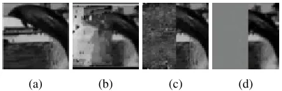
(a) (b) (c) (d)
Figure 6: DCSPNs performed well on a dataset with 65 im-ages. Left-completion of the original image in (a) by DC-SPN (b), P&D (c), and DCGAN (d).
age local structure in the image data in both directions. Fifth, accuracy was improved by using height-by-width instead of a 1-by-1 filter, that is, no sharing of parameters was more effective than sharing parameters. A similar finding was ob-served in (Sharir et al. 2018).
DCSPNs left-complete well on a small dataset. The Cal-tech Dolphin dataset only contains 65 images. Nevertheless, DCSPNs performed quite well, as exemplified by the MSE scores in Table 2 and by the left-completions illustrated in Figure 6.
On the contrary, DCSPN completions admittedly look as though they are sometimes composed of random blocks of high frequency. To mitigate this, a low pass Gaussian fil-ter can be applied as a smoothing post-processing step. This simple technique lowers the DCSPN MSE score in Olivetti left-completion in Table 1 from 455 to401.
We also tried other common CNN techniques, such as average-pooling instead of sum-pooling layers, sharing pa-rameters in convolutional layers, batch normalization, and dropout, but did not observe any significant improvement. It is noted that dropout was successfully applied in SPNs for image classification (Peharz et al. 2018).
DCSPNs with Differentiable MPE
Motivated by future work suggested in (Vergari et al. 2018), we propose an alternative method of training DCSPNs that is based on differentiable MPE. Whereas (5) minimizes the negative log-likelihood loss function, the new training method also considers the error between the given input and the MPE assignment (completion).More formally, letD(x)be the value of a DCSPNDwith inputx. LetY⊆Xand consider inputy, where the value of each variable inY is 1, namely, the variables inY are marginalized out. The MPE assignment after both forward and backward propagation inDis denoted byM(y). Then, the objective function for trainingDcan be defined as:
min
M maxD E[log D(x)] +E[log(1−D(M(y)))]. (6)
Using (6) to train DCSPNs yields an MSE score of651for left-completion in the Olivetti dataset. This beats all compet-ing scores in Table 1, except for DCSPNs trained uscompet-ing (5). Training DCSPNs using (6) is intriguing for more than sim-ply a promising MSE score.
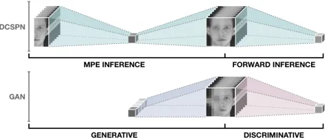
Figure 7: MPE and forward inference in SPNs are similar to the generator and discriminator in GANs, respectively.
a simple distribution such as a normal distribution.G up-sampleszand outputs G(z). The discriminatorDreceives
G(z)or dataset samplesxand downsamples to a classifica-tion output. Hence, training GANs involves minimizingG
and maximizingD:
min
G maxD E[log D(x)] +E[log(1−D(G(z)))]. (7)
Figure 7 illustrates a general relationship between training DCSPNs with differentiable MPE in (6) and GANs training in (7). Observe that MPE inference computingM(y)in (6) plays the role of the generatorGin GANs computingG(z)in (7). However, while the GANs generatorGupsamples noise to form an image, DCSPNs use MPE inference to upsample the network value to form an image.
Similarly, forward inference in DCSPNs computingD(x) in (6) assumes the part of the discriminator in GANs computingD(x)in (7). Hence, DCSPN forward inference downsamples to a log-likelihood value measuring how likely the given input is from the sample distribution, whereas the GANs discriminator downsamples to a classification of whether or not the input data is real.
On the other hand, the GANs generator has its own learn-able parameters, since the generator and discriminator are two different networks. However, a DCSPN is a single net-work, resulting in the sharing of parameters during learning between MPE inference and forward inference. Further in-vestigation of DCSPNs with differentiable MPE and its re-lationship to GANs training remains as future work.
Image Sampling
DCSPNs can sample images by modifying Algorithm 1. In-stead of selecting a maximizing child, randomly select a child. More formally, replace lines 19 and 20 to instead as-sign values toCby randomly sampling from a categorical distribution parameterized by the convolutional layer filter weights. Note that the forward pass is no longer needed.
The sampled images in Figure 8 are encouraging as vari-ability is evident. Moreover, these results were obtained in an inaugural attempt at DCSPN image sampling involving a minor modification to Algorithm 1. Some generative mod-els, including GANs, are known for low variability due to mode collapse(Metz et al. 2017; Salimans et al. 2016).
Figure 8: DCSPN image sampling shows variability.
Related Works
Here we comment on other vectorized approaches to SPNs. (Poon and Domingos 2011) and (Vergari, Di Mauro, and Esposito 2015) have discussed relationships between CNNs and SPNs. The interpretation of an SPN sum layer depends on the type of probabilistic inference being conducted. For marginal inference, an SPN sum layer corresponds to a con-volutional layer in CNNs. For MPE, on the other hand, an SPN sum layer corresponds to a max-pooling layer in CNNs. We extend the literature by showing that an SPN product layer can correspond to a sum-pooling layer in CNNs.
(Sharir et al. 2018) introduced a tractable generative model, calledconvolutional arithmetic circuits(ConvACs). An arithmetic circuit (Darwiche 2003) is a deep learning model that has been shown by (Rooshenas and Lowd 2014) to be equivalent to SPNs. In particular, ConvACs include a representation layer(Sharir et al. 2018). We found this in-troduction useful in practice. However, similar to CSPNs, ConvACs may suffer from being shallow.
(Peharz et al. 2018) suggest an SPN learning method in-volving a discriminative and generative loss function. Al-though the generative part is also based on the log-likelihood similar to (6), the discriminative part is different. They con-sider the cross-entropy function of the SPN parameters, while we introduced to notion of a minmax game using dif-ferentiable MPE.
Conclusion
Deep convolutional sum-product networks (DCSPNs) can form rich DAG structures of convolutional and sum-pooling layers, while still being valid SPNs. As a tractable generative model, DCSPNs can perform efficient probabilistic reason-ing, including marginal inference and approximate MPE in-ference. On the other hand, as a CNN, DCSPNs can build deeper structures using both vertical and horizontal sum-pooling windows, which leverage local structure in the im-age data. Practical applications of DCSPNs include imim-age completion and image sampling. DCSPNs are flexible in that they allow for an alternative learning method based on differentiable MPE. Relationships between this learning ap-proach and learning in GANs are discussed.
References
Amos, B.; Xu, L.; and Kolter, J. Z. 2017. Input convex neural networks. InProceedings of the Thirty-Fourth Inter-national Conference on Machine Learning (ICML 2017). Amos, B. 2016. Image Completion with Deep Learn-ing in TensorFlow. http://bamos.github.io/2016/08/09/ deep-completion. Accessed: July 1st, 2018.
Conaty, D.; Mau´a, D.; and de Campos, C. P. 2017. Approx-imation complexity of maximum a posteriori inference in sum-product networks. InProceedings of the Thirtieth Con-ference on Uncertainty in Artificial Intelligence (UAI 2017). Darwiche, A. 2003. A differential approach to inference in Bayesian networks.Journal of the ACM (JACM)50(3):280– 305.
Delalleau, O., and Bengio, Y. 2011. Shallow vs. deep sum-product networks. InProceedings of the Twenty-Fourth Con-ference on Neural Information Processing Systems (NIPS 2011), 666–674.
Dennis, A., and Ventura, D. 2012. Learning the architecture of sum-product networks using clustering on variables. In Proceedings of the Twenty-Fifth Conference on Neural In-formation Processing Systems (NIPS 2012), 2033–2041. Fei-Fei, L.; Fergus, R.; and Perona, P. 2007. Learning gen-erative visual models from few training examples: An incre-mental Bayesian approach tested on 101 object categories. Computer Vision and Image Understanding106(1):59–70. Goodfellow, I.; Bengio, Y.; and Courville, A. 2016. Deep Learning. MIT Press.
Goodfellow, I.; Pouget-Abadie, J.; Mirza, M.; Xu, B.; Warde-Farley, D.; Ozair, S.; Courville, A.; and Bengio, Y. 2014. Generative adversarial nets. In Proceedings of the Twenty-Seventh Conference on Neural Information Process-ing Systems (NIPS 2014), 2672–2680.
He, K.; Zhang, X.; Ren, S.; and Sun, J. 2016. Deep resid-ual learning for image recognition. InProceedings of the IEEE Conference on Computer Vision and Pattern Recogni-tion (CVPR 2016), 770–778.
Kingma, D. P., and Ba, J. 2014. Adam: A method for stochastic optimization.arXiv preprint arXiv:1412.6980. Kingma, D. P., and Welling, M. 2014. Auto-encoding vari-ational Bayes. InProceedings of the International Confer-ence on Learning Representations (ICLR 2014).
Larochelle, H., and Murray, I. 2011. The neural autore-gressive distribution estimator. InProceedings of the Four-teenth International Conference on Artificial Intelligence and Statistics (AISTATS 2011), 29–37.
Metz, L.; Poole, B.; Pfau, D.; and Sohl-Dickstein, J. 2017. Unrolled generative adversarial networks. Proceedings of the International Conference on Learning Representations (ICLR 2017).
Oord, A. v. d.; Kalchbrenner, N.; and Kavukcuoglu, K. 2016. Pixel recurrent neural networks. InProceedings of the Inter-national Conference on Machine Learning (ICML 2016). Peharz, R.; Tschiatschek, S.; Pernkopf, F.; and Domingos, P. 2015. On theoretical properties of sum-product networks. In
Proceedings of the Eighteenth International Conference on Artificial Intelligence and Statistics (AISTATS 2015), 744– 752.
Peharz, R.; Gens, R.; Pernkopf, F.; and Domingos, P. 2017. On the latent variable interpretation in sum-product net-works.IEEE Transactions on Pattern Analysis and Machine Intelligence39(10):2030–2044.
Peharz, R.; Vergari, A.; Stelzner, K.; Molina, A.; Trapp, M.; Kersting, K.; and Ghahramani, Z. 2018. Probabilistic deep learning using random sum-product networks. arXiv preprint arXiv:1806.01910.
P´erez, P.; Gangnet, M.; and Blake, A. 2003. Poisson image editing. ACM Transactions on Graphics (TOG)22(3):313– 318.
Poon, H., and Domingos, P. 2011. Sum-product networks: A new deep architecture. In Proceedings of the Twenty-Seventh Conference on Uncertainty in Artificial Intelligence (UAI 2011), 337–346.
Rooshenas, A., and Lowd, D. 2014. Learning sum-product networks with direct and indirect variable interactions. In Proceedings of the Thirty-First International Conference on Machine Learning, 710–718.
Salimans, T.; Goodfellow, I.; Zaremba, W.; Cheung, V.; Rad-ford, A.; and Chen, X. 2016. Improved techniques for training gans. InProceedings of the Thirtieth Annual Con-ference on Neural Information Processing Systems (NIPS 2016), 2234–2242.
Samaria, F. S., and Harter, A. C. 1994. Parameterisation of a stochastic model for human face identification. In Pro-ceedings of the Second IEEE Workshop on Applications of Computer Vision (WACV 1994), 138–142.
Sharir, O.; Tamari, R.; Cohen, N.; and Shashua, A. 2018. Tensorial mixture models. arXiv preprint arXiv:1610.04167.
Vergari, A.; Peharz, R.; Di Mauro, N.; Molina, A.; Kerst-ing, K.; and Esposito, F. 2018. Sum-product autoencoding: Encoding and decoding representations using sum-product networks. InProceedings of the Thirty-Second AAAI Con-ference on Artificial Intelligence (AAAI 2018), 4163–4170. Vergari, A.; Di Mauro, N.; and Esposito, F. 2015. Simpli-fying, regularizing and strengthening sum-product network structure learning. In Proceedings of the Joint European Conference on Machine Learning and Knowledge Discov-ery in Databases (ECML PKDD 2015), 343–358.
Vergari, A.; Di Mauro, N.; and Esposito, F. 2016. Vi-sualizing and understanding sum-product networks. arXiv preprint arXiv:1608.08266.