Eigenvalue Approach to Generalized
Thermoelastic Interactions in an Annular Disk
N. Gangopadhyaya#1,N. C. Das#2
1
Department of Mathematics, Calcutta Institute of Engineering and Management, Kolkata-700040, India. 2
Department of Mathematics, Brainware Group of Institutions, Kolkata-700124, India.
Abstract: The present paper encompasses the analytical solution for axisymmetric one dimensional thermomechanical response of an annular disk. The basic equations have been written in the form of a vectormatrix differential equation in the Laplace transform domain and solved by eigenvalue approach. The solutions for displacement, temperature, radial and hoop stresses are obtained in closed form in the Laplace transform domain. Numerical inversions for these field variables in the space-time domain have been made and presented in graphical form.
Keywords: Generalized thermoelasticity, Thermomechanical response, Annular disk, Eigenvalue approach, Laplace transform.
I. INTRODUCTION
The unrealistic prediction that the thermal disturbances propagate at infinite speed as given in the classical theory of thermoelasticity based on conventional heat conduction equation, some modified dynamic thermoelastic models are proposed by some researchers which encompasses the notion that not only the equations of motion but also the heat conduction equation must be of hyperbolic type and as such the elastic wave and heat wave propagate in finite speed. This modified thermoelastic theory is known as Generalized theory of thermoelasticity. Lord and Shulman [1], based on a modified Fourier law, developed a generalized theory (L-S theory) where they used a relaxation time parameter. Green and Lindsay [2], based on an entropy production inequality, which was put forwarded by Green and Laws [3], developed a temperature rate dependent thermoelasticity (G-L theory) that includes the temperature-rate among constitutive variables also predicts a finite speed for heat propagation where they have used two time relaxation parameters. Another theoretical model on this area is due to Green and Nagdhi [4, 5] (G-N theory) who provide sufficient basic modifications in the constitutive equations that permit treatment of a much wider class of heat flow problems. The applications of these theories have been examined extensively by a host of researchers and to name a few vide, [6-12]. The problems of generalized thermoelasticity with phase-lag effects are also being considered by the researchers, vide, [13-16].
Bagri and Eslami [17] applied the finite element method to solve the problem of generalized coupled thermoelastic disk based on LS model [1]. Taheri, et.al [18] presented the thermoelastic analysis of an annulus using GN-model. Kar and Kanoria [19] considered the thermoelastic response in a fiber reinforced thin annular disk with three phase-lag effect. Following Bagri and Eslami [17], we have considered the thermoelastic interactions in an annular disk using eigenvalue approach to achieve the solution. Finally, the displacement, temperature, radial and hoop stresses are inverted from the transform domain to the space time domain by numerical method and presented graphically. The results are also compared with the corresponding results as in [17].
II. BASIC EQUATIONS AND CONSTITUTIVE RELATIONS
We consider an isotropic homogeneous annular disk of inner radius and outer radius having initially at a uniform temperature , under axisymmetric thermal shock load applied into its inner boundary. The disk is assumed to be in plane
stresscondition and the origin in plane polar coordinates is taken at the centre of the hole.
Following L-S model [1], the linear coupled equations of motion and generalized heat conduction equation in terms of displacement and temperature and in absence of heat source and body forces can be written in plane-stress condition as
22
2
grad div
u
curl curl
u
grad
T
u
t
(1) 2 2 20 2 0 0 2
div
0
e e
T
T
k
T
c
c t
T
t
u
t
t
t
t
(2)
The stress-strain-temperature relations can be written as
div
2
ij
u
ije
ijT
ij
(3) For plane-stress condition, we write2
2
, =
2
2
(4) where are the Lame constants and are the density, stress tensor, referencetemperature, stress temperature module, thermal conductivity, specific heat and relaxation time parameter respectively.
We now consider an annular disk under axisymmetric thermal shock load applied to its inner boundary of the disk.
Writing the equations (1) - (3) in plane coordinates and assuming that
( , ),
0 and
( , )
u
u r t
v
w
T
T r t
we write these equations (1) - (3) as
2 22 2 2
1
1
2
u
T
u
r
r r
r
r
t
(5)2 3 2 2
0 0 0
2 2 2
1
1
1
1
0
e
k
c
t
T
T t
u
r
r r
t
t
r t
r t
r t
r t
(6)
2
1
1
rru
T
u
u
r
u
r
r
T
r
(7)In order to make the above equations in dimensionless form, we introduce the dimensionless parameters as
0 1 1
0
0 0 0
2
,
tc
,
t c
,
,
u
,
r
T
qt
r
t
t
T
u
q
t
t
t
T
t T
kT
(8)where 2 1 1
2
,
ek
l
c
c c
Employing these dimensionless parameters and neglecting the prime notation for convenience, equations (5) – (7) become
2 2
2 2 2
1
1
0
T
u
r
r r
r
t
r
(9)2 3 2 2
0 0
2 2 2
1
1
1
1
t
T
C t
u
0
r
r r
t
t
r t
r t
r t
r t
(10)
2
1
1
1
1
2
2
rr
u
u
u
r
T
u
r
r
r
(11)
where is the thermoelastic coupling coefficient. It may be noted from the equations (9) and (10) that the
elastic wave propagates with the speed to unity and the thermal disturbance propagates with the speed of . Since
finite speed is predicted for the generalized L-S model. Otherwise when , infinite speed of thermal disturbance is
estimated for classical thermoelastic case.
The mechanical and thermal boundary conditions for the annular disk may be taken as
1
2
1
2
0 at
0 at
and
at
0 at
rr
u
r
r
r
r
T
k
q t
r
r
r
T
r
r
(12)
Using the relations (8), the dimensionless forms of the equation (12) may be written as
0 ,
at
0 ,
0 at
rr
T
u
q
r
a
r
T
r
b
(13)
where , is a constant and is the Heaviside unit step function of t for the heat flux input at the
inner boundary and a, b are the dimensionless inner and outer radii respectively.
III. SOLUTION OF THE PROBLEM
We now apply Laplace transform of the function with parameter defined by
0
pt
f p
e
f t dt
to the equations (9) – (10) and get 2
2
2 2
1
d u
du
u
dT
p u
dr
r dr
r
dr
(14)
2
0 0
2
1
1
1
d T
dT
du
u
p
t p T
Cp
t p
dr
r dr
dr
r
(15) Equations (14) can be written as
2dT
L u
p u
dr
(16)Differentiating (15) with respect to „
r
‟ and using the equation (16) we get
2
0
1
1
dT
dT
L
p
t p
Cp u
C
dr
dr
(17) where the operatorL
is given by2
2 2
1
1
d
d
L
dr
r dr
r
Equations (16) and (17) may be combined to write in the vector-matrix differential equation form as
2
3
0 0
1
1
1
1
u
u
p
L dT
dT
Cp
t p
p
C
t p
dr
dr
This equation may be written as
Lv
Av
(18)where 11 12 11 2 12 21 3
0
22
0
21 22
,
,
,
1,
1
,
1
1
u
a
a
v
dT
A
a
p
a
a
Cp
t p
a
p
C
t p
a
a
dr
In order to solve the equation (18), we follow the procedure as in [20].
Let be the eigenvectors corresponding to the eigenvalues of the matrix and let
1
A V V
where 1
1 2
20
,
0
V
V
V
(19)Equation (18) becomes
1
Lv
V V
v
(20) Premultiplying by , equation (20) may be written as
1 1L V v
V v
or,
L y
y
, where
y
V v
1
or,
v
V y
(21)Writing (say), we get from (19) and (21)
Ly
1
1 1y
and
Ly
2
2y
2(22) We write equations (22) in the form
2
2 2
1
1
- (
)
0,
1, 2
m m
m m
d y
dy
y
m
dr
r dr
r
(23)Writing (say), (24)
the solution of equation (23) can be written as
1
(
)
1(
),
1, 2
m m m m m
y
A K
r
B I
r
m
(25)where are the modified Bessel functions of the second kind and are constants.
The eigenvalues of the matrix A can be determined from the characteristic equation:
2
11 22 11 22 21 12
- (
a
a
)
(
a a
-
a a
)
0
(26)Then can be written as
12 12
1 11 2 11
a
a
V
a
a
(27)Using (25), we now write down as
1 1 1
(
1)
1 1(
1)
y
A K
r
B I
r
(28)2 2 1
(
2)
2 1(
2)
y
A K
r
B I
r
(29)Thus, from (21), since we obtain
12 12 1
2 2
1 11 2 11 2
u
a
a
y
dT
a
a
y
dr
Hence, we get the displacement and temperature in the Laplace transform domain as
,
1 1(
1)
1 1(
1)
2 1(
2)
2 1(
2)
u r p
A K
r
B I
r
A K
r
B I
r
(30)
2 12 2 12 2 22 2 221 0 1 1 0 1 2 0 2 2 0 2
1 1 2 2
,
p
(
)
p
(
) +
p
(
)
p
(
)
T r p
A
K
r
B
I
r
A
K
r
B
I
r
(31) Using (30) and (31), we calculate the radial and hoop stresses as
1 2 0 1 1 1 1 2 0 1 1 11 1
2 2
2 0 2 1 2 2 0 2 1 2
2 2
1
2
1
2
,
(
)
(
)
(
)
(
)
2
2
1
2
1
2
(
)
(
)
(
)
(
)
2
2
rr
p
p
r p
A
K
r
K
r
B
I
r
I
r
r
r
p
p
A
K
r
K
r
B
I
r
I
r
r
r
(32)
2 121 1 0 1 1 1
1
2 2
1
1 1 0 1 1 1
1
2 2
2
2 2 0 2
2
1
2
,
(
)
(
)
2
2
1
2
(
)
(
)
2
2
(
2
p
r p
A
K
r
K
r
r
p
B
I
r
I
r
r
p
A
K
r
1 22 2
2
2 2 0 2 1 2
2
1
2
)
(
)
2
1
2
(
)
(
)
2
2
K
r
r
p
B
I
r
I
r
r
(33)We now use the boundary conditions (13) to determine the constants . The resulting equations are as follows:
11 1 12 1 13 2 14 2
21 1 22 1 23 2 24 2 0
31 1 32 1 33 2 34 2
41 1 42 1 43 2 44 2
0
0
0
C A
C B
C A
C B
C A
C B
C A
C B
H
C A
C B
C A
C B
C A
C B
C A
C B
(34) where
2 211 1 1 12 1 1 13 1 2 14 1 2 21 1 1 1
2 2 2 2 2 2
22 1 1 1 23 2 1 2 24 2 1 2
2 2 2 2
1 1
32 0 1 32 0 1
1 1
(
),
(
),
(
),
(
),
(
),
(
),
(
),
(
),
(
),
(
),
C
K
a
C
I
a
C
K
a
C
I
a
C
p p
K
a
C
p p
I
a
C
p p
K
a
C
p p
I
a
p
p
C
K
b
C
I
b
2 2 233 0 2
2
2 2 2
2
34 0 2 41 0 1 1 1
2 1
2 2
42 0 1 1 1 43 0 2 1 2
1 2
2
44 0 2
2
=
(
),
1
2
(
),
(
)
(
),
2
1
2
1
2
(
)
(
),
(
)
(
),
2
2
1
2
(
)
2
p
C
K
b
p
p
C
I
b
C
K
b
K
b
b
p
p
C
I
r
I
b
C
K
b
K
b
b
b
p
C
I
r
b
1(
2)
I
b
Solving this system of equations for the constants and substituting them in the equations (30) – (33) we get
the displacement, temperature and stresses in the Laplace transform domain as
1 1 1 2 1 1 3 1 2 4 1 2
1
,
(
)
(
)
(
)
(
)
u r p
K
r
I
r
K
r
I
r
(35)
2 12 2 12 2 221 0 1 2 0 1 3 0 2
1 1 2
2 2
2
4 0 2
2
1
,
(
)
(
) +
(
)
(
)
p
p
p
T r p
K
r
I
r
K
r
p
I
r
(36)
1 2 0 1 1 1 2 2 0 1 1 11 1
2 2
3 0 2 1 2 4 0 2 1 2
2 2
1
1
2
1
2
,
(
)
(
)
(
)
(
)
2
2
1
2
1
2
(
)
(
)
(
)
(
)
2
2
rr
p
p
r p
K
r
K
r
I
r
I
r
r
r
p
p
K
r
K
r
I
r
I
r
r
r
(37)
2 121 1 0 1 1 1
1
2 2
1
2 1 0 1 1 1
1
2 2
2 3
1
1
2
,
(
)
(
)
2
2
1
2
(
)
(
)
2
2
p
r p
K
r
K
r
r
p
I
r
I
r
r
p
2 0 2 1 22
2 2
2
4 2 0 2 1 2
2
1
2
(
)
(
)
2
2
1
2
(
)
(
)
2
2
K
r
K
r
r
p
I
r
I
r
r
(38) where11 12 13 14 12 13 14 11 13 14
21 22 23 24 0 22 23 24 21 0 23 24
1 2
31 32 33 34 32 33 34 31 33 34
41 42 43 44 42 43 44 41 43 44
0
0
,
,
,
0
0
0
0
C
C
C
C
C
C
C
C
C
C
C
C
C
C
H
C
C
C
C
H
C
C
C
C
C
C
C
C
C
C
C
C
C
C
C
C
C
C
C
C
C
C
11 12 13
11 12 14
21 22 23 0
21 22 0 24
3 4
31 32 33
31 32 34
41 42 43
41 42 44
0
0
,
0
0
0
0
C
C
C
C
C
C
C
C
C
H
C
C
H
C
C
C
C
C
C
C
C
C
C
C
C
C
IV. FOR SOLID DISK
Instead of choosing an annular disk, we now choose a solid disk of radius with centre at the origin.
In this case, the boundary conditions may be taken as
0,
on
rr
dT
q
r
b
dr
(39)Since is undefined for , we write the solution for displacement and temperature in the Laplace
transform domain as
,
1 1(
1)
2 1(
2)
u r p
B I
r
B I
r
(40)
2 12 2 221 0 1 2 0 2
1 2
,
p
(
)
p
(
)
T r p
B
I
r
B
I
r
(41)
1 2 0 1 1 1 2 2 0 2 1 21 2
1
2
1
2
,
(
)
(
)
(
)
(
)
2
2
rr
p
p
r p
B
I
r
I
r
B
I
r
I
r
r
r
(42)
2 121 1 0 1 1 1
1
2 2
2
2 2 0 2 1 2
2
1
2
,
(
)
(
)
2
2
1
2
(
)
(
)
2
2
p
r p
B
I
r
I
r
r
p
B
I
r
I
r
r
(43)Applying the boundary conditions (39), we calculate the constants and which when substituted in (40) – (43), give
, ,
rrand
u T
for the solid disk as
1 1 1 2 1 2
1
,
(
)
(
)
u r p
I
r
I
r
(44)
2 12 2 221 0 1 2 0 2
1 2
1
,
p
(
) +
p
(
)
T r p
I
r
I
r
(45)
1 2 0 1 1 1 2 2 0 2 1 21 2
1
1
2
1
2
,
(
)
(
)
(
)
(
)
2
2
rr
p
p
r p
I
r
I
r
I
r
I
r
r
r
(46)
2 121 1 0 1 1 1
1
2 2
2
2 2 0 2 1 2
2
1
1
2
,
(
)
(
)
2
2
1
2
(
)
(
)
2
2
p
r p
I
r
I
r
r
p
I
r
I
r
r
(47)where 11 12 11 22 12 21 0 12 0 22 11 0 0 21
21 22 22 21
,
,
0
0
C
C
H
C
C
H
C C
C C
H C
H C
C
C
C
C
2 2
2 2
11 1 1 1
,
12 2 1 2,
C
p p
I
b
C
p p
I
b
2 2
21 0 1 1 1 22 0 2 1 2
1 2
1
2
1
2
(
)
(
),
(
)
(
)
2
2
p
p
C
I
b
I
b
C
I
b
I
b
b
b
, ,, V. NUMERICAL RESULTS
In order to illustrate the preceding results graphically, we have chosen the material aluminium for numerical evaluation. As in [17] the material constants are taken as
The first four figures represent the wave propagation of temperature, radial displacement, radial stress and hoop stress along the radial direction where we have considered the numerical values of the relaxation time and coupling parameter as 0.64 and
0.02 respectively.
Figure 1 predicts the wave propagation of temperature along the radial direction for different values of time . It is noticed that
the temperature at assume the maximum value of 0.2181, 0.3863, 0.519, 0.6268, 0.7168 and 0.7926 at = 0.2, 0.4, 0.6,
0.8, 1.0 and 1.2 respectively. The maximum temperature occurs for = 1.2 at . The figure shows that at time = 0.2,
0.4, 0.6 the thermal wave propagates through the radius of the disk and it is reflected from the outer boundary of the disk at times = 0.8, 1.0 and 1.2 respectively.
Figure 2 represents the radial displacement when increases. At the stipulated values of time as mentioned in Figure1, it
is seen that the maximum displacement for = 0.2, 0.4, 0.6, 0.8, 1.0 and 1.2 are 0.005625 at = 1.09, 0.02011 at = 1.21,
0.04101 at = 1.3, 0.06651 at = 1.39, 0.09524 at = 1.49 and 0.1608 at = 1.98 respectively. It is also noticed that the
curves related to times = 0.2, 0.4, 0.6 and 0.8 show the propagation of displacement waves whereas those related to = 1.0
and 1.2 show the reflection of same waves from the outer boundary of the disk.
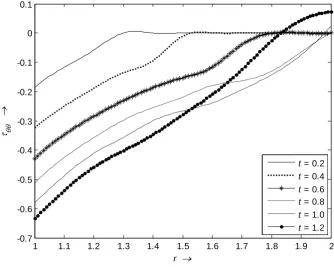
The natures of the radial stress and hoop stress have been presented in Figure 3 and Figure 4 respectively. For both the figures it is noticed that the reflection of waves change from contraction to tensile at the outer boundary of the disk since the outer boundary is stress free.
Figure 3 and Figure 4 represent the radial and hoop stress distribution along the radial direction for different values of time. As time increases the magnitude of the stress at the wave front also increases whereas the gradient decreases.
Figure 5 – Figure 8 gives the time variation of temperature, displacement, radial stress and hoop stress at the middle of the disk for different values of relaxation time with coupling coefficient taken as 0.02.
From Figure5 it is observed that as relaxation time increases from 0.64 to 1.5625 the peak value of temperature also increases in the range , thereafter the temperature decreases to the minimum 0.278 at = 2.68 for = 0.64. The curve for
temperature for = 1.5625 predicts the minimum value of 0.2509 at = 4.31.
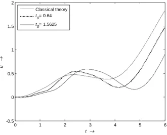
Graphs of similar nature as in Figure5 have been exhibited by the displacement as presented in Figure6.
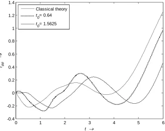
From Figure7 it is seen that for the relaxation time = 0.64, the minimum values are -0.3211, 0.06008, -0.209 at = 1.05,
1.95 and 4.03 respectively and maximum values of 0.06118, 0.1075, 0.5739 are attained at = 0.12, 1.66 and 2.68. For =
1.5625, the minimum values are -0.2631, 0.03827 and -0.2475 at = 1.31, 2.28 and 4.77 respectively whereas the maximum
values are 0.006349, 0.07122, 0.5397 at = 0.36, 2.01 and 3.18.
Hoop stress as presented in Figure8 shows the graphs of similar nature as in Figure 7.
In order to compare our results for temperature, displacement and stresses as presented by graphs in Figure 5 – Figure 8 with the corresponding field variables for the classical case, we have presented curves by dashed lines in each of the figure.
We now consider the case of the solid disk in which we have deduced the equations for displacement, temperature, radial stress and hoop stress in equations (44) – (47).
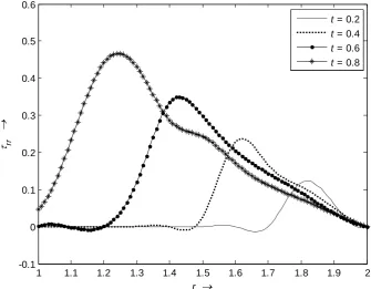
In the present paper we would present the graph of the radial stress versus variation of radial distance for some stipulated time
. In this case the coupling coefficient and the relaxation time are assumed to be 0.02 and 0.64 respectively. It is noticed from
Figure 9 that the radial stress in each case first increases nearly from zero to a maximum value and then decreases to zero as
increases. The peak values of are respectively 0.466 at = 1.24 for = 0.8, 0.3497 at = 1.43 for = 0.6, 0.2374 at =
1.62 for = 0.4, 0.1229 at = 1.82 for = 0.2.
Our graphs of temperature, displacement, radial stress and hoop stress in figures (1) to (8) are in complete agreement in nature with the corresponding figures (1) to (8) of Bagri and Eslami [17] who obtained the solution of the problem through finite element method.
1 1.1 1.2 1.3 1.4 1.5 1.6 1.7 1.8 1.9 2 -0.1
0 0.1 0.2 0.3 0.4 0.5 0.6 0.7 0.8
r
T
t = 0.2
t = 0.4
t = 0.6
t = 0.8
t = 1.0
t = 1.2
Figure1. The temperature distribution along the radius of the disk
1 1.1 1.2 1.3 1.4 1.5 1.6 1.7 1.8 1.9 2 -0.02
0 0.02 0.04 0.06 0.08 0.1 0.12 0.14 0.16 0.18
r
u
t = 0.2
t = 0.4
t = 0.6
t = 0.8
t = 1.0
t = 1.2
Figure2. The displacement distribution along the radius of the disk
1 1.1 1.2 1.3 1.4 1.5 1.6 1.7 1.8 1.9 2 -0.35
-0.3 -0.25 -0.2 -0.15 -0.1 -0.05 0 0.05 0.1
r
rr
t = 0.2
t = 0.4
t = 0.6
t = 0.8
t = 1.0
t = 1.2
Figure3. The radial stress distribution along the radius of the disk
1 1.1 1.2 1.3 1.4 1.5 1.6 1.7 1.8 1.9 2 -0.7
-0.6 -0.5 -0.4 -0.3 -0.2 -0.1 0 0.1
r
t = 0.2
t = 0.4
t = 0.6
t = 0.8
t = 1.0
t = 1.2
Figure 4. The hoop stress distribution along the radius of the disk
0 1 2 3 4 5 6 -0.1
0 0.1 0.2 0.3 0.4 0.5 0.6
t
T
Classical theory
t
0= 0.64
t0= 1.5625
Figure 5. The temperature variation at middle of disk for different values of relaxation time
0 1 2 3 4 5 6
-0.5 0 0.5 1 1.5 2
t
u
Classical theory
t0= 0.64
t0= 1.5625
Figure 6. The displacement variation at middle of disk for different values of relaxation time
0 1 2 3 4 5 6 -0.4
-0.2 0 0.2 0.4 0.6 0.8 1 1.2 1.4 1.6
t
rr
Classical theory
t
0= 0.64
t
0= 1.5625
Figure 7. The radial stress variation at middle of disk for different values of relaxation time
0 1 2 3 4 5 6
-0.4 -0.2 0 0.2 0.4 0.6 0.8 1 1.2 1.4
t
Classical theory
t
0= 0.64
t
0= 1.5625
Figure 8. The hoop stress variation at middle of disk for different values of relaxation time
1 1.1 1.2 1.3 1.4 1.5 1.6 1.7 1.8 1.9 2 -0.1
0 0.1 0.2 0.3 0.4 0.5 0.6
r
rr
t = 0.2
t = 0.4
t = 0.6
t = 0.8
Figure 9. The radial stress distribution along the radius of the solid disk
VI. CONCLUSIONS
In this paper, we consider generalized theory of thermoelasticity with one relaxation time parameter (Lord Shulman model) to investigate the thermomechanical response of an annular disk as well as solid disk. In order to invert the field variables
( , ), ( , ),
rr( , ),
( , )
u r p
T r p
r p
r p
as in equations (35) to (38) and (44) to (47) from Laplace transform domain tospace-time domain, we consider Zakian‟s algorithm [21] technique. The distributions of temperature, displacement, radial and hoop stresses are plotted along the radial direction for different values of time. Also the effects of relaxation time on the field variables are exhibited. The wave front for temperature is detected from Fig.1 and the elastic wave fronts are detected from Fig.3 and Fig.4. Also the effects of relaxation time on the field variables are exhibited. Finally, the radial stress along the radial direction for different values of time for solid disk is presented graphically.
REFERENCES
[1] H.W.Lord, Y.Shulman, “A Generalized Dynamical Theory of Thermoelasticity”, J.Mech.Phys.Solids, vol.15, pp.299-309, 1967. [2]A.E.Green, K.A.Lindsay, “Thermoelasticity”, J.Elasticity, vol.2, pp.1-7, 1972.
[3]A.E.Green, N.Laws, “On The Entropy Production Inequality”, Arch.Rat.Mech.Anal, vol.45, pp.45-47, 1972.
[4]A.E.Green, P.M.Nagdhi, “A Re-examination of The Basic Postulates of Thermodynamics”, Proc.R.Soc. London A, vol.432, pp.171-194, 1991. [5] A.E.Green, P.M.Nagdhi, “Thermoelasticity without Energy Dissipation”, J.Elasticity, vol.31, pp. 189-208, 1993.
[6]R.B.Hetnarski, J.Ignaczak, “Generalized Thermoelasticity”, J.Thermal Stresses, vol.22, pp.451-476, 2004.
[7]D.S.Chandrasekharaiah,” Hyperbolic Thermoelasticity: A review of Recent Literature”, Appl.Mech.Review, vol.51, pp.705-729, 1998. [8]M.Anwar, H.Sherief, “State Space Approach to Generalized Thermoelasticity”, J.Thermal Stresses, vol.11, pp.353-365, 1988.
[9]N.C.Das, A.Lahiri, “Thermoelastic Interactions Due to Prescribed Pressure Inside a Spherical Cavity in an Unbounded Medium”, Int. J. Pure and Appl.Math., vol.31, pp.19-32, 2001.
[10]H.Sherief, “On Uniqueness and Stability in Generalized Thermoelasticity”, Quarterly of Appl.Math., vol.45, pp.773-778, 1987. [11]J. Ignaczak , “Uniqueness in Generalized Thermoelasticity”, J.Thermal Stresses, vol.2, pp.171-175, 1979.
[12]H. M. Youssef, “Theory of Two-Temperature Generalized Thermoelasticity”, IMA J.Appl.Math, vol.71, pp.383-390, 2006.
[13]S.Banik, M.Kanoria, “Effects of Three-Phase-Lag on Two-Temperature Generalized Thermoelasticity for Infinite Medium with Spherical Cavity”, Appl. Math. Mech-Engl.Ed., vol.33, pp.483-498, 2012.
[14]R.Quintanilla, R. Racke, “A Note on Stability in Three-Phase Lag Heat Conduction, International “, J. Heat and Mass Transfer, vol. 51, pp.24-29, 2008. [15]R. Kumar, S. Mukhopadhyay, “Analysis of The effects of Phase-lags on Propagation of Harmonic Plane Waves in Thermoelastic Media”, Comp. Methods in Science and Technology, vol.16, pp.19-28, 2010.
[16] R. Kumar, S. Mukhopadhyay, “Effects of Three-Phase Lags on Generalized Thermoelasticity for an Infinite Medium with a Cylindrical Cavity”, J.Thermal stresses, vol.32, pp.1149-1165, 2009.
[17]A. Bagri, M. R. Eslami, “Generalized Coupled Thermoelasticity of Disks Based on The Lord-Shulman Model”, J.Thermal Stresses, vol.27, pp.691-704, 2004.
[18]H.Taheri, S.J.Fariborz, M.R.Eslami, “Thermoelastic Analysis of an Annulus Using the Green-Nagdhi Model”, J.Thermal Stresses, vol.28, pp.911-927, 2005.
[19]A. Kar, M.Kanoria, “ Analysis of Thermoelastic Response in a Fiber Reinforced Thin Annular Disc with Three-Phase-Lag Effect”, European J.of Pure and Applied Math, vol.4, pp.304-321, 2011
[20]A.Lahiri, N.C.Das, S.Sarkar and M.Das, “Matrix Method of solution of Coupled Differential Equations and Its Applications in Generalized Thermoelasticity”, Bull. Calcutta Mathematical Society, vol.101, pp.571-590, 2009.
[21]V.Zakian, “ Inversion of Laplace Transforms”, Electronic Letters, vol.5, pp.120-121, 1969.