A Particle-Based Variational Approach to Bayesian
Non-negative Matrix Factorization
Muhammad A Masood [email protected]
Harvard John A. Paulson
School of Engineering and Applied Science Cambridge, MA 02138, USA
Finale Doshi-Velez [email protected]
Harvard John A. Paulson
School of Engineering and Applied Science Cambridge, MA 02138, USA
Editor:Francois Caron
Abstract
Bayesian Non-negative Matrix Factorization (BNMF) is a promising approach for under-standing uncertainty and structure in matrix data. However, a large volume of applied work optimizes traditional non-Bayesian NMF objectives that fail to provide a principled understanding of the non-identifiability inherent in NMF—an issue ideally addressed by a Bayesian approach. Despite their suitability, current BNMF approaches have failed to gain popularity in an applied setting; they sacrifice flexibility in modeling for tractable computation, tend to get stuck in local modes, and can require many thousands of samples for meaningful uncertainty estimates. We address these issues through a particle-based variational approach to BNMF that only requires the joint likelihood to be differentiable for computational tractability, uses a novel transfer-based initialization technique to iden-tify multiple modes in the posterior, and thus allows domain experts to inspect a small set of factorizations that faithfully represent the posterior. On several real datasets, we obtain better particle approximations to the BNMF posterior in less time than baselines and demonstrate the significant role that multimodality plays in NMF-related tasks.
Keywords: Bayesian, Non-negative Matrix Factorization, Stein discrepancy, Non-identifiability, Transfer Learning
1. Introduction
The goal of non-negative matrix factorization (NMF) is to find a rank-RNMF factorization
for a non-negative data matrixX (Ddimensions byN observations) into two non-negative factor matrices A and W. Typically, the rank RNMF is much smaller than the dimensions
and observations (RNMF D, N).
X≈AW | X ∈RD+×N, A∈R
D×RNMF
+ , W ∈R
RNMF×N
+
The linear, additive structure of these non-negative factor matrices makes NMF a popular unsupervised learning framework for discovering and interpreting latent structure in data. Each observation in the data X is approximated by an additive combination of the RNMF
columns of A with the combination weights given by the column of W corresponding to
c
that observation. In this way, the basis matrix A provides a part-based representation of the data and the weights matrixW provides anRNMF-dimensional latent representation of
the data under this part-based representation.
The ability to easily interpret NMF solutions in this way has made them appealing in many applied areas. A few applications of NMF include understanding protein-protein interactions (Greene et al., 2008), topic modeling (Roberts et al., 2016), hyperspectral un-mixing (Bioucas-Dias et al., 2012), polyphonic music transcription (Smaragdis and Brown, 2003), discovering molecular pathways from genomic samples (Brunet et al., 2004), and summarizing activations of a neural network for greater interpretability (Olah et al., 2018). However, the analysis and interpretation of latent structure in a dataset via NMF is affected by the possibility that several non-trivially different pairs ofA, W may reconstruct the dataXequally well. This non-identifiability of the NMF solution space has been studied in detail in the theoretical literature (Pan and Doshi-Velez, 2016; Donoho and Stodden, 2003; Arora et al., 2012; Ge and Zou, 2015b; Bhattacharyya et al., 2016), and domain experts using NMF as a tool have noticed this issue as well. Greene et al. (2008) use ensembles of NMF solutions to model chemical interactions, while Roberts et al. (2016) conduct a detailed empirical study of multiple optima in the context of extracting topics from large corpora.
Bayesian approaches to NMF promise to characterize this parameter uncertainty in a principled manner by solving for the posteriorp(A, W|X) given priorp(A, W) and likelihood
p(X|A, W) e.g. Schmidt et al. (2009); Moussaoui et al. (2006). Having a representation of uncertainty in the parameters of the factorizations can assist with the proper interpretation of the factors, allowing us to place low or high confidence on parameters of the factorization. However, computational tractability of inference limits the application of the Bayesian ap-proach. Uncertainty estimates obtained from current Bayesian methods are often of limited use: variational approaches (e.g. Paisley et al. (2015); Hoffman and Blei (2015)) typi-cally underestimate uncertainty and fit to a single mode; sampling-based approaches (e.g. Schmidt et al. (2009); Moussaoui et al. (2006)) also rarely switch between multiple modes and often require many thousands of samples for meaningful uncertainty estimates.
As a result of the limitations of current Bayesian approaches, domain experts tend to rely on non-Bayesian approaches to characterize uncertainty in NMF parameters. For example, Greene et al. (2008); Roberts et al. (2016); Brunet et al. (2004) all use random restarts to find multiple solutions.1 Random restarts have no Bayesian interpretation (as they depend on the basins of attraction of each mode), but they do often find multiple optima in the objective that can be used to understand and interpret the data.
Contributions In this work, we present a transfer-learning approach that remains faithful to a principled Bayesian framework and can efficiently identify multiple, disconnected modes for any differentiable prior and likelihood model. Our transfer-learning based approach provides high-quality and diverse NMF initializations to seed a particle-based approximation to the Bayesian NMF (BNMF) posterior. We demonstrate our inference approach on two different BNMF models: first, the common exponential-Gaussian model; second, a novel
model that corresponds more closely with the desires of domain experts. Through our experiments, we demonstrate that:
• On a large number of real-world datasets, our particle-based posterior approximations consistently outperform baselines in terms of both posterior quality and computational running time.
• Our approach allows us to produce relatively small (less than 100 NMFs) sets of par-ticles that belong to multiple modes of the posterior landscape, have distinct inter-pretations, and exhibit variability in performance on downstream tasks—all of which may be essential for a domain expert to inspect and understand the full solution space.
• Our novel practitioner-friendly BNMF model involves a new scale-fixing prior that removes many uninteresting multiple optima and captures the kinds of loss-insensitive regions that are important in many applications. Inference in this non-conjugate model is significantly more challenging than with more standard BNMF models, but our approach handles this case with ease.
2. Inference Setting
The general process of Bayesian modeling consists of three main parts. First, we must select a model (a likelihood and prior). Next, we perform inference on the model given data (under some objective). Finally, we evaluate the quality of the inference. The main innovation in this work is a novel transfer-based approach to the inference phase (Section 4). Along the way, we also introduce a novel model for BNMF that is more closely aligned to what domain experts desire from NMFs (Section 5.2).
When performing inference, we must choose how we will approximate the true posterior
p(A, W|X). For notational simplicity, letθrepresent NMF parameters (A, W). We approxi-mate the full BNMF posteriorp(θ|X) with a discrete variational distributionq(θ|θ1:M, w1:M)
that has M different point-masses θm. Each θm represents a different NMF solution’s full
set of parameters: θm = vec[ATm, Wm], and is assigned probability masswm. The functional
form of the variational distribution is given by:
p(θ|X)≈q(θ|θ1:M, w1:M) = M X m=1
wmδ(θ−θm)
s.tw1:M ∈∆M−1, where θm= vec[ATm, Wm]
(1)
whereδis the Dirac delta distribution and ∆M−1is the probability simplex inRM.
Particle-based approximations are attractive to domain experts because each sample represents something that they can inspect and understand.
Section 3) now enables us to measure the quality of anarbitrary finite collection as a poste-rior approximation.2 As such, it opens the door to entirely new classes of particle-generation techniques, where traditional conditions, such as detailed balance, are now replaced with minimizing the Stein discrepancySp(q)3 between the true BNMF posterior p(θ|X) and the
discrete approximationq(θ|θ1:M, w1:M):
q∗(θ|θ1:M, w1:M) = argminq(θ|θ1:M,w1:M)Sp(θ|X)(q(θ|θ1:M, w1:M)) s.t.w1:M ∈∆
M−1 (2)
As with all variational inference problems, the problem of posterior inference is now reduced to the problem of optimizing the objective above; we are free to explore any method for producing settings{θ1:M, w1:M} to minimize the Stein discrepancy to the true posterior.
In the following, we observe that the task of minimizing this Stein discrepancy often depends on producing high-quality, diverse factorization collections θ1:M and determining
their associated weightsw1:M. In Section 4, we introduce a transfer-learning based approach
to efficiently suggest a diverse collection of particles and optimize their associated weights. We describe traditional BNMF as well as a novel threshold-based NMF model, and discuss their merits in the context of our approach in Section 5. Experimental details including parameter choices for our approach as well as description of baselines and evaluation metrics is provided in Section 6. In Section 7, we compare our approach to more traditional particle-based approaches (MCMC), more naive ways of generating candidate particle collections, as well as directly attempting to optimize the Stein objective above. We evaluate the quality of different posterior approximations both based on their Stein discrepancies, likelihoods and reconstruction on held-out data.
3. Background
Bayesian Non-negative Matrix Factorization In BNMF, we define a prior p(A, W) and a likelihood p(X|A, W) and seek to characterize the posterior p(A, W|X). These are related by Bayes’ rule:
p(A, W|X) = p(X|A, W)p(A, W)
p(X)
There exist many options for the choice of prior and likelihood (e.g., exponential-Gaussian, (Paisley et al., 2015; Schmidt et al., 2009), Gamma Markov chain priors (Dikmen and Cemgil, 2009) and volume-based priors (Arngren et al., 2011)). The likelihood and prior choices are often chosen to have good computational properties (e.g. the resulting partial conjugacy of the exponential-Gaussian model). One advantage of our work is that we do not require the computationally convenient priors for inference.
Transfer learning The field of transfer learning aims to leverage models and inference applied to one problem to assist in solving related problems. It is of practical value because
2. While the popular Kullback-Leibler divergence requires comparing the ratio of probability densities or probability masses, the Stein discrepancy can be used to compare a particle-based collection defined by probability masses with a continuous target distribution.
3. This notation refers to the Stein discrepancy (a variational objective) between two distributionspand
there may be an abundance of data and computational resources for one problem but not another (see Pan and Yang (2010) for a survey). In this work, we shall use the solutions to BNMF from small, synthetic problems to help solve much larger NMF problems.
Stein discrepancy The Stein discrepancy Sp(q) is a divergence from distributions q(θ)
to p(θ) that only requires sampling from the variational distribution q(θ) and evaluating the score function of the target distributionp(θ). The Stein discrepancy is computed over some class of test functions f ∈ F and satisfies the closeness property for operator vari-ational inference (Ranganath et al., 2016): it is non-negative in general and zero only for some equivalence class of distributions q ∈ Q0. For a rich enough function class, the only distribution for which the Stein discrepancy is zero is the distributionp itself. For discrete distributions like ourq(θ|θ1:M, w1:M) from Section 2, the approximation quality to the
pos-terior distributionp(θ|X) of interest can be analytically computed using recent advances in Stein discrepancy evaluation with kernels (Liu and Feng, 2016; Chwialkowski et al., 2016; Gretton et al., 2006; Liu et al., 2016; Gorham and Mackey, 2015). The Stein discrepancy is related to the maximum mean discrepancy (MMD): a discrepancy that measures the worst-case deviation between expectations of functions h ∈ H under p and q (Gretton et al., 2006).
MMD(H, q, p) := sup
h∈HEθ
∼q[h(θ)]−Eθ0∼p[h(θ0)]
The Stein operator Tp corresponding to the distribution p is given by
(Tph)(x) :=
1
p(x)h∇, p(x)h(x)i
and under its application, the function space His transformed into another function space
Tp(H) =F. The advantage of applying this operator to the MMD equation is that expec-tations under p of any f ∈ F are zero, i.e. Eθ0∼pf(θ0)) = 0 (Barbour and Brown, 1992).
The Stein discrepancy is given by:
Sp(H, q) := sup f∈Tp(H)
(Eθ∼qf(θ))2
Computing the Stein discrepancy is of particular interest when the distribution p is intractable. Evaluating the Stein discrepancy does not require expectations overp and the Stein operator Tp only depends on the unnormalized distribution via the score function ∇θlogp(θ).
In this work, we use a kernelized form of the Stein discrepancy. For every positive definite kernel k(θ, θ0), a unique Reproducing Kernel Hilbert Space (RKHS) H is defined. Chwialkowski et al. (2016) showed that the Stein operator applied to an RKHS defines a modified positive definite kernel Kp given by:
Kp(θ, θ0) =∇θlogp(θ)T∇θ0logp(θ0)k(θ, θ0)
+∇θ0logp(θ0)T∇θk(θ, θ0)
+∇θlogp(θ)T∇θ0k(θ, θ0)
+
d X
i=1
∂2k(θ, θ0)
∂θi∂θi0
Finally, the Stein discrepancy is simply the expectation of the modified kernelKp under the joint distribution of two independent variables θ,θ0 ∼q.
Sp(q) =Eθ,θ0∼q[Kp(θ, θ0)]
For a discrete distribution over θ1:M with probability masses w1:M (of the form in
equa-tion 1), this can be evaluated exactly (Liu and Lee, 2016) as:
Sp(q) = M X i,j=1
wiwjKp(θi, θj)
=wTKw
(4)
The (pure) quadratic formwTKwis a reformulation where K∈RM×M is the (positive
definite) pairwise kernel matrix with entries Kij = Kp(θi, θj) and the probability masses
w1:M are embedded into a vector w ∈ RM×1. Our particle-based variational objective
(equation 2) simplifies to the form in equation 4. In Section 4, we will provide a method for estimatingθ1:M and w1:M for the BNMF problem.
4. Approach
In this Section, we describe our transfer-based inference. As noted in Section 2, creating a particle-based posterior involves two distinct parts: creating a collection of candidate NMFs
θ1:M, and then optimizing their weightsw1:M. We introduce a novel transfer-based approach
that uses state-of-the-art (non-Bayesian) algorithms to efficiently generate the candidate NMFs θ1:M (Section 4.1). Given θ1:M, we optimize the weights w1:M via standard convex
optimization tools to minimize Stein discrepancy. (See Algorithm 1 for the full algorithm.) In Section 7, we compare our approach for generating candidate NMFs and weights to other baselines, including those that use traditional methods for particle generation (MCMC), other ways of creating candidate NMFs (and then again using a convex optimization on the weights), and gradient-based optimization of the objective.
4.1. Learning factorization parameters θ1:M via Transfer Learning
A natural approach to finding the factorization parameters θ1:M is to optimize for them
directly via the variational objective (equation 2), however, as we shall see in Section 7, the direct approach tends to get stuck in poor local optima and is computationally expensive. Since the quality of the variational approximation is determined solely by the value of the variational objective under a given set of parametersθ1:M,w1:M, we are free to employ any
technique that produces a suitable collectionθ1:M.
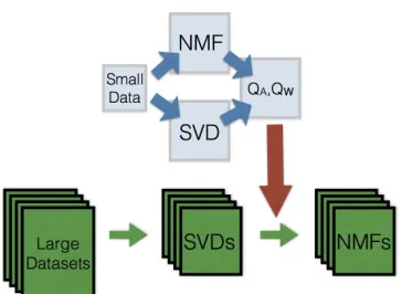
Figure 1: A schematic of the transfer learning procedure for NMF: A small dataset is used to learn transformation matricesQA, QW. We then apply these transformation matrices to
multiple larger datasets (with any number of dimensions or observations) using its SVD to obtain a transfer-based initialization.
convergence of these methods (Salakhutdinov et al., 2002; Wild et al., 2004; Xue et al., 2008; Boutsidis and Gallopoulos, 2008). However, these random restarts do not take advantage of any structure of NMF; for each new NMF instance they propose random initializations from scratch. As such, many initializations may converge to the same mode—a waste of computational effort—while missing other modes (especially when the number of restarts is small).
In this Section, we introduce a transfer-based technique (which we will callQ-Transform) to speed-up, as compared to random restarts, the process of finding a diverse set of fac-torizations from high-density regions of the posterior. Our initializations are determined by identifying the low-rank subspace of the data (via singular value decomposition (SVD)) and then transforming it in specific ways. Figure 1 shows a schematic illustrating the idea: we generate subspace transformation matrices QA, QW from a number of small,
syn-thetic datasets and then apply those transformations to the dataset of interest. These transformations serve as more intelligent initializations—compared to random restarts— from which to apply NMF algorithms to obtain a more diverse collection of high-quality NMFs. Because our initializations are almost always already decent NMFs, convergence is also computationally faster. To explain our Q-Transform procedure, we first define the subspace transformation matrices, then describe the method for generating transformation matrices QA, QW using synthetic data, and finally discuss how to apply them to real data
sets (transfer learning).
Subspace transformations QA, QW relating SVD and NMF A low dimensional
approximation for the data X can be obtained via the top RSVD vectors of the SVD ASVD, WSVD. An NMFA, W of rankRT (which may be different fromRSVD) also leads to
an approximation of the data. The NMF factors are interpretable due to the non-negativity constraint whereas the SVD factors typically violate non-negativity. However, both ap-proaches describe low dimensional subspaces that can be used to understand and approxi-mate the data. These subspaces are the same whenRSVD =RT and the NMF is exact (i.e.
Algorithm 1 Particle-based Variational Inference for BNMF usingQ-Transform
Input: Data{X}, Rank{RNMF}, # Factorizations M
Step 1: PerformM repetitions of Algorithm 2 to get matrices {QmA, QmW}M
m=1 or re-use
them if previously constructed
Step 2: ApplyQ-Transform (Algorithm 3) to get Initializations {Am0 , W0m}M m=1 Step 3: Apply NMF algorithm to get Factorizations {Am, Wm}M
m=1
Step 4: Apply Algorithm 5 using a given BNMF model to get weights {wm}M m=1 for
approximate posterior
Output: Discrete NMF Posterior {wm, Am, Wm}M m=1
these conditions, there exist transformation matrices QA, QW to obtain the non-negative
basis and weights exactly in terms of the singular value decomposition matrices:
If X =ASVDWSVD=AW then A=ASVDQA W =QWWSVD
When the data X is not an exact NMF but rather a perturbation of it (i.e. X =
AW+), the singular subspace of the matrix is bounded by Wedin’s theorem (Wedin, 1972). We therefore still expect that there exist transformation matrices QA∈ RRSVD×RT, Q
W ∈ RRT×RSVDto yield approximations of the NMF factorizations that can be expressed in terms
of the singular value decomposition matrices.
AQ=ASVDQA≈A WQ=QWWSVD ≈W
Our transfer-based strategy will involve identifying candidate matricesAQ∈RD×RT, W
Q∈ RRT×N such thatASVDQAandQWWSVD are likely to be good initializations for an NMF of
the dataX. (Note that we assume that computing the SVD to obtainASVDandWSVDfrom
the data X is straight-forward.) We will describe the details for using these initializations below, but first we describe how we might create a collection of candidate transformation matrices QA, QW.
Generating transformations QA, QW for NMF initialization. To generate
candi-date transformations, we note that if we have already computed an NMF A, W for a dataset X, the appropriate transforms QA, QW can be computed by relating the SVD
factorsASVD, WSVD toA, W (e.g. via linear least squares). We propose to generate
candi-date transforms by using random restarts on small, synthetic datasetsXs that follow some
generative model for NMF, where we can run (non-Bayesian) NMF algorithms quickly and solve forQA, QW (Algorithm 2). Multiple pairs of transformation matrices can be obtained
by repeating Algorithm 2 with different random initializations to compute NMF of the synthetic dataXs, as well as by generating multiple synthetic datasets (see Section 8.1 for
experiments and discussion of alternate generation procedures). Since the transformations
QA, QW act on the inner dimensions (columns of ASVD and rows of WSVD), we emphasize
Algorithm 2 GenerateQ-Transform Matrices
Input: Synthetic Data{Xs}, SVD Dimension{RSVD}, Transfer Dimension{RT}
ASVD, WSVD ← Compute topRSVD SVD of Xs
ANMF, WNMF ← Compute rank-RT NMF of Xs using random initialization
QA= arg min Q
kANMF−ASVDQkF via linear least squares
QW = arg min Q
kWNMF−QWSVDkF via linear least squares Output: QA,QW
Algorithm 3 ApplyQ-Transform
Input: Real Data {X}, SVD Rank {RSVD}, NMF Rank {RNMF}, Transformation
Ma-trices {QA, QW}
ASVD, WSVD ← Compute topRSVD SVD of X
˜
A0=ASVDQA, W˜0 =QWWSVD
A0, W0 ←Apply non-negativity and fix dimensions: Algorithm 4 ( ˜A0,W˜0, RNMF) Output: A0,W0
Creating initializations for a new dataset. Given the top SVD factors of a new datasetASVD, WSVD, we apply theQ-Transform (Algorithm 3) which multiplies SVD factors
by the QA, QW matrices and adjusts entries of ASVDQA and QWWSVD to ensure
non-negativity and correct dimensions using Algorithm 4 to obtain initializationsA0, W0that can
be used as input for any standard (non-Bayesian) NMF algorithm (e.g. Cichocki and Phan (2009), F´evotte and Idier (2011)). Algorithm 4 ensures that all values in the initialization
A0, W0 are non-negative as well as provides a way to pad the initialization if the size RT
of the transforms QA, QW are smaller than the desired NMF rank RNMF. The latter is
an important point: in Section 8.3 we find that it is often the first few dimensions of the transformation that contain transferable information, and the rest provide little benefit. This observation also allows us to use transforms of some rankRT on problems with a range
of desired NMF ranksRNMF. Finally, running the algorithm gives us a set of factorization
parameters θm = vec[ATm, Wm] that we may (or may not) ultimately decide to keep in our
approximation of the true posterior.
In the experiments in Section 7, we find that knowledge from these transformations
QA, QW can be transferred to real datasets by re-using them to relate the top SVD factors
of other datasets to high quality, approximately non-negative factorizations.4
4.2. Learning weights w1:M given parameters θ1:M
To infer the weights corresponding to a given factorization collection θ1:M, we minimize
the Stein discrepancy (Algorithm 5) subject to the simplex constraint on the weights. This process involves first computing the pairwise kernel matrix5 Kusing the kernelKp in equa-tion 3. The objective funcequa-tion is convex and can be solved using standard convex optimiza-tion solvers. Given point-masses θ1:M, this framework can be employed to infer weights
Algorithm 4 Initialization Adjustment
Input: Approximation matrices {AQ, WQ}, NMF Rank {RNMF}
˜
A0←Absolute Value(AQ)
˜
W0←Absolute Value(WQ)
Transfer Rank RT = # Columns ofAQ
if NMF RankRNMF >Transfer RankRT then
r=RNMF−RT
Pad ˜A0,W˜0 with matrices MD×r and MN×r having small random entries so that
ini-tializations are the correct dimensions and matrices MD×r, MN×r have little effect of
the product ˜A0W˜0. A0 ←[ ˜A0, MD×k]
W0 ←[ ˜W0 T
, MN×k]T
else if NMF Rank RNMF <Transfer RankRT then
Pick the top RNMF columns of ˜A0 and rows of ˜W0 A0 ←A˜0[:,0 :RNMF]
W0 ←W˜0[0 :RNMF,:] end if
Algorithm 5 Kernelized Stein inference for discrete approximations to posterior
Input: Particlesθ1:M, Score∇θlogp(θ), RKHS H defined by kernelk Step 1: Compute pairwise kernel matrix Ki,j =Kp(θi, θj) (from equation 3)
Step 2: Find probability masses that minimize the Stein discrepancy for the given point-masses: w∗ = arg minwwTKw s.t. w∈∆M−1 via standard convex optimization.
Output: Probability masses w∗
for discrete approximations to any posterior for which the score function∇θlogp(θ) can be computed.
5. BNMF Models
Section 4 outlined a general procedure for producing a particle-based approximation to the BNMF posterior using transfer learning. In Section 7, we compare our approach to other particle-based approaches for BNMF. However, before going to the results, we first describe the two BNMF models (below) as well as our experimental procedure (Section 6).
differences are small compared to the magnitude of the likelihood may be considered similar by a practitioner (Roberts et al., 2016). Our threshold-based likelihood model allows the practitioner to choose what levels of error are effectively the same for their purposes.
Before continuing, we emphasize again that our transfer-based inference approach can be applied to any BNMF model; in this paper we demonstrate our approach on the follow-ing two models because together they include a standard model often-used in the machine learning community and a novel model of interest to the practitioner community. Impor-tantly, because our inference approach decouples the process of model choice, particle gen-eration, and particle weighting, we use the same particle generation process (non-Bayesian optimization algorithms using the Frobenius objective) for both models. In Section 7, we demonstrate empirically that this particle generation process is robust enough; that is, we do not require processes tuned to each model.
5.1. Exponential-Gaussian Model for BNMF
The commonly used exponential-Gaussian BNMF model uses a Gaussian likelihood and exponential priors for the basis and weights matrices:
pN(X|A, W) =
Y d,n
N(Xd,n,(AW)d,n, σX2 )
p(A) =
D Y d=1 R Y r=1
p(Ad,r), Ad,r ∼Exp(λd,r)
p(W) =
N Y n=1 R Y r=1
p(Wr,n), Wr,n∼Exp(λr,n)
As derived in Schmidt et al. (2009), the combination of exponential priors and Gaussian likelihoods results in element-wise conjugate parameter updates; in general, this model enjoys relatively straightforward inference approaches.
That said, as noted above, the exponential-Gaussian has several drawbacks from the perspective of a domain expert seeking to interpret their data via NMF. First, especially in settings where the model is misspecified (which will almost always be the case), the recon-struction error of even the best factorization may be relatively large. Even so, the Gaussian likelihood will tend to make the posterior highly peaked around the MAP solution—and exclude factorizations of only slightly worse (relative approximation) quality with respect to the overall error. However, domain experts may have found those factorizations inter-esting, as they have about the same relative error. Second, the exponential prior allows for some amount of uncertainty simply due to scale, which is typically uninteresting for domain experts. In the following, we introduce a model that addresses both of these shortcomings; because our transfer-based inference approach does not require conjugacy, we will be able to efficiently compute approximate posteriors for such more complex models.
5.2. Threshold-based, Scale-Fixing Model for BNMF
the joint density p(X, W, A) to be differentiable in order to make inference tractable. Such flexibility is important as different applied domains use different notions of factorization quality: squared Euclidean distance is commonly used in hyperspectral unmixing (Bioucas-Dias et al., 2012), Kullback-Leibler divergence in image analysis (Lee and Seung, 2001) and Itakura-Saito divergence in music analysis (F´evotte et al., 2009).
A common theme in many applied domains is that small differences in factorization qual-ity may not be important if all factorizations have some large level of approximation error. In such cases, domain experts may be interested in all of these solutions (Roberts et al., 2016). At the same time, solutions that are different only in scale are likely uninteresting. Below, we present a novel prior and likelihood that reflect these application-specific prefer-ences of practitioners in a Bayesian framework. In particular, our model class allows domain experts to take any application-specific notion of a high-quality factorization—conjugate or not—and put it into a Bayesian context.
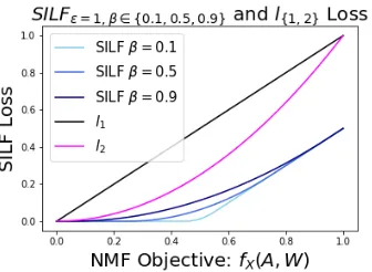
Likelihood: Soft Insensitive Loss Function (SILF) over NMF objectives We define a likelihood that is maximum (and flat) in the region of high quality factorizations and decays as factorization quality decreases. To do so, we use the soft insensitive loss function (SILF) (Chu et al., 2004): a loss function defined over the real numbersR, where
the loss is negligible in some region around zero defined by the insensitivity threshold , and grows linearly outside that region (see figure 2). A quadratic term depending on the smoothness parameterβ, makes the transition between the two main regions smooth. This transition region has length 2β, making smaller values ofβcorrespond to sharper transitions between the flat and linear loss regions. We adapt the SILF from (Chu et al., 2004) to only be defined over the non-negative numbersR+(as is typical with NMF objectives) and define
it as:
SILF,β(y) =
0 0≤y ≤(1−β) (y−(1−β))2
4β (1−β)≤y≤(1 +β)
y− y ≥(1 +β)
To form the likelihood, we apply the SILF loss to an NMF objectivefX(A, W) to give:
P(X|W, A) = 1
Ze
(−C×SILF,β(fX(A,W))) (5)
We emphasize that the SILF-based likelihood allows the domain expert to use an NMF objectivefX(A, W) that is best suited to their task and can specify a threshold under that
objective for identifying high-quality factorizations. Once an NMF objective is chosen, the domain expert can easily choose appropriate parameters for the SILF-based likelihood since the parameters (insensitivity factorand smooth transition factor β) are interpretable and the likelihood can be visually inspected (as a one-dimensional function of a chosen NMF objective) to validate parameter choices.
Figure 2: A comparison of SILF loss and commonly used l1, l2 loss functions. The SILF
insensitivity parameter is set to 0.5, and the smooth transition factor β is varied. Small values of β lead to sharp transition in the SILF loss profile whereas the transition is less abrupt for large values ofβ. In contrast, other popular loss functions such asl1 orl2 do not
have insensitive regions, and in the case of NMF, treat the objective function as the sole guide for factorization quality.
that is uninteresting in practice:
AW =ASP | {z } e
A
(SP)−1W | {z }
f
W
where S is a positive diagonal matrix, P is a permutation matrix
(6)
Depending on the priors chosen, this ambiguity can add redundancy to the posterior dis-tribution.
To facilitate exploration of the space of distinct high-quality factorizations, we propose an NMF prior that eliminates redundancy due to scale and is also uniform over the space of factorizations. Specifically, we let each column of the basis matrix Ar be generated by
a symmetric Dirichlet distribution with parameter α = 1. This prior determines a unique scale of the factorization and is uniform over the basis matrixAfor that scaling. ForW, we use a prior where each entryWr,n is i.i.d from an exponential distribution with parameter
λr,n. The exponential distribution has support over allR+ensuring that any weights matrix W corresponding to a column-stochastic basis matrix A is a valid parameter setting under our model, and that the posterior is proper.
p(A) =
R Y r=1
p(Ar), Ar ∼Dir(1D)
p(W) =
N Y n=1 R Y r=1
p(Wr,n), Wr,n∼Exp(λr,n)
6. Experimental Setup
array of benchmark NMF datasets as well as on Electronic Health Records (EHR) data of patients with Autism Spectrum Disorder (ASD) that is of interest to the medical community (see quantitative and qualitative results in Section 7).
6.1. Model, Evaluation, and Inference Settings
Model: exponential-Gaussian model parameters: We set the standard deviation
σX to be equal to the empirical standard deviation of a reference NMF. The exponential
parameter was set to one for each entry in the basis and weights matrices (λd,r =λr,n= 1).
Model: SILF model parameters: While any objective can be put into the SILF likeli-hood, in the following, we used the squared Frobenius objectivefX(A, W) =kX−AWk2F.
To set the threshold parameter for each dataset, we use an empirical approach where we find a collection of 50 high-quality factorizations under default settings of scikit-learn (Pedregosa et al., 2011). The objective function is evaluated for each of them {fi}50i=1 and = 1.2 maxifi. We set the remaining SILF likelihood sensitivity parameters β = 0.1,
C= 2. For the prior, we identically set the exponential parameter for each entry: λr,n= 1.
Inference: Generating Q-transform matrices for transfer: For the Q-Transform initializations, we set the transfer rank and SVD rank RT = RSVD = 3. We generated
twenty sets of synthetic data Xs ∈ R12+×12 using non-negative matrices of rank RT with
truncated Gaussian noise. For each synthetic dataset, we find five pairs of transformation matrices through random restarts. In all our experiments, the same set of Mmax = 100
pairs of transformation matrices {QmA, QmW}100
m=1 are applied to each of the real datasets. Inference: Solver for inferring weights w1:M: The optimization for the weightsw1:M
(Step 2 in Algorithm 5) is carried out using the Splitting Conic Solver (SCS) in the convex optimization package CVXPY (Diamond and Boyd, 2016).
Inference and evaluation: Stein discrepancy base RKHS and parameters: The Stein discrepancy for our variational objective requires a function space to optimize over. This optimization over the function space has an analytical solution when a Reproducing Kernel Hilbert Space (RKHS) is used. Gorham and Mackey (2017) show that the Inverse Multiquadric (IMQ) kernel is a suitable kernel choice for Stein discrepancy calculations as it detects non-convergence to posterior6 forc >0 and b∈(−1,0).
kIMQ(θi, θj) = (kθi−θjk2+c2)b
Since the length scales of the basis and weights matrix differ, we define a kernel via a linear combination of two IMQ kernels defined separately over the basisA and weightsW.
k([A1, W1],[A2, W2]) =
1 2γA
(kA1−A2k2+c2A)bA+
1 2γW
(kW1−W2k2+c2W)bW (7)
Here γA = (c2A)bA and similarly γW = (c2W)bW are scaling factors that ensure the kernel
takes values between 0 and 1. In general, across our datasets, the Dirichlet prior on the
basis matrix induces a small length scale forAand a larger length scale for the weights W. We uniformly setcA= 1×10⁻²,cW = 1×10³ andbA=bW =−0.5 across all our datasets.
We note that choosing sensible values for these parameters—and validating them—is important. Kernel parameters that induce length scales that are too small or too large give rise to a similarity measure that either considers all factorizations completely dissimilar or completely similar respectively. In our experiments, our kernel choice gives rise to a simi-larity measure that distinguishes across collections of factorizations obtained from different algorithms. Our kernel similarity analysis shows agreement with difference between factor-izations as measured by the Frobenius distances between basis and weights matrices (see figures 24, 25, 26 in Appendix). The range in kernel similarity values and its agreement with alternative measures indicates that our parameter choices for the kernel are reasonable and fairly robust.7
Evaluation: Measuring computational time In experiments, we keep track of the time taken (initialization and optimization) to produce each of the Mmax = 100
factoriza-tions. We sample collections of size M = {5,25,50} from these factorizations and report the total time taken to produce the factorizations in the collection alongside reporting the Stein Discrepancies for the approximate BNMF posteriors.
For the baselines below, the reported runtimes correspond to time taken to generate NMFs{θm}Mm=1in the approximate posterior. For initialization approaches this corresponds
to the time taken to generate the initialization and subsequent optimization time. To allow for a transparent comparison of the performance of these initialization approaches with MCMC and gradient-based algorithms, we report runtimes at various points in the duration of the MCMC chain and for the gradient-based algorithms. For more details on measuring computational time, see Appendix E in supplementary materials.
6.2. Baselines
In the previous Section, we described the implementation details for our transfer-based inference approach. In this Section, we describe implementation details for three classes of baselines for our experiments: MCMC, which represents standard practice for generat-ing particle-based posteriors; gradient-based approaches which directly minimize the Stein variational objective, which represent our main competitors; and alternate initialization approaches, which represent simpler ablations on our approach.
Markov Chain Monte Carlo baselines MCMC approaches involve sampling from a Markov Chain whose stationary distribution is the posterior of interest, and are often consid-ered the gold-standard for approximating posterior distributions (as opposed to variational methods). That said, for a finite sample size, MCMC will still be approximate—and thus we must still evaluate its quality with respect to the Stein objective. In this work, we consider two different MCMC baselines:
• Hamiltonian Monte Carlo (HMC) Our HMC was initialized with an NMF ob-tained using the default settings of scikit-learn (Pedregosa et al., 2011) (warm start), and adaptively selects the step-size using the procedure outlined in Neal et al. (2011).
We run the chain for a total of 10000 samples and at various intermediate points thin it to M = {5,25,50} factorizations and compute the Stein discrepancy using Algorithm 5. We repeat this experiment three times to capture variability in the performance of the HMC.
For our scale-fixing prior in Section 5.2, we needed to simulate Hamiltonian dy-namics as defined on the manifold of the simplex. To do this, we incorporate a reparametrization trick (Betancourt, 2012; Altmann et al., 2014) to sample under the column-stochastic (simplex) constraints of the basis matrix A, and a mirroring trick (Patterson and Teh, 2013) for sampling from the positive orthant for the weights matrixW.
• Gibbs Sampling. Only the exponential-Gaussian model admits a conjugate form for straight-forward Gibbs sampling. For experiments using the exponential-Gaussian, we use the same number of samples and thinning factor as with HMC for a Gibbs sampler. Similarly to the HMC baseline, the Gibbs sampler was also initialized with an NMF obtained using the default settings of scikit-learn (Pedregosa et al., 2011) (warm start).
Gradient-based baselines Gradient-based baselines optimize the collection of factor-izations directly via gradient descent on the Stein variational objective. They represent the class of inference approaches most similar to ours. Gradient-based approaches typically require fixing the size of the collection. In our experiments, we set the size of this collection to be equal toM = 5. Due to the large memory requirement of running this algorithm with automatic differentiation using autograd (Maclaurin et al., 2015), we were unable to run these algorithms for largerM. We impose scaling and non-negativity constraints after every gradient step (for a total of 2000 steps) and keep track of the Stein discrepancy in relation to the algorithm’s runtime. The experiment is repeated three times to capture variability in its performance over multiple iterations. We use the following three algorithms:
• SVGD: Stein Variational Gradient Descent is a functional gradient descent algorithm (Liu and Wang, 2016) that optimizes a collection of particles (factorizations) to ap-proximate the posterior. We replace the RBF kernel from the original work with the more principled IMQ-based kernel defined in equation 7.
• SVGD-Qis a variant were we initialize SVGD with theQ-Transform.
• DSGD: Direct Stein Gradient Descent is a variant where we replace the functional gradient descent of SVGD with the gradient of the Stein discrepancy (using automatic differentiation (Baydin et al., 2015; Maclaurin et al., 2015)).
Initialization-based baselines Our Q-transform approach can be thought of as an ini-tialization approach: we provide a way of creating a collection of particles that we believe are likely to be representative of the posterior. Our main algorithm can be run with any pro-cess for creating the collection (step 2 of Algorithm 1). Our final set of baselines considers other alternatives to creating the collection.
from a truncated standard normal distribution. These entries are all scaled by η =
q 1 RNMF
P
D,NXd,n and are given by: A0d,k, Wk,n0 ∼η|N(0,1)|.
• NNDSVDar NNDSVDar is a variant of a popular initialization technique called Nonnegative Double Singular Value Decomposition (NNDSVD) which was introduced by Boutsidis and Gallopoulos (2008). It is based on approximating the SVD expansion with non-negative matrices. Since the NNDSVD algorithm is deterministic, this only gives a single initialization. The NNDSVDar variant of this initialization replaces the zeros in the NNDSVD initialization with small random values. We use the scikit-learn initialization for NNDSVDar which uses a randomized SVD algorithm (Halko et al., 2011), and note that it introduces some additional variability in the initializations.
6.3. Datasets
Our datasets cover a range of different types and can be divided into three main categories (count data, grayscale face images and hyperspectral images). The ranks for hyperspectral data are chosen according to ground truth values. In the 20-Newsgroups data, we select articles from 16 newsgroups (hence the rank 16) and for other datasets we pick a rank that corresponds to explaining at least 70 percent of the variance in the data (as measured by the SVD). Table 1 provides a description of each dataset as well as the rank used and a citation. The Autism dataset is of interest to the medical community for understanding disease subtypes in the Autism spectrum and is not publicly available. The remaining datasets are public and are considered standard benchmark datasets for NMF. In our experiments, we hold out ten percent of the observations and report performance on both provided and held-out observations.
Table 1: Datasets for NMF
Dataset Dimension Observations Rank Description
20-Newsgroups 1000 8926 16 Newspaper articles (20NG, 2013) Autism 2862 5848 20 Patient visits (Doshi-Velez et al., 2014)
LFW 1850 1288 10 Grayscale Faces Images (LFW, 2017)
Olivetti Faces 4096 400 10 Grayscale Faces Images (Samaria, 1994) Faces CBCL 361 2429 10 Grayscale Faces Images (CBCL, 2000) Faces BIO 6816 1514 10 Grayscale Faces Images (Jesorsky et al., 2001) Hubble 100 2046 8 Hyperspectral Image (Nicolas Gillis, 1987) Salinas A 204 7138 6 Hyperspectral Image (SalinasA, 2015) Urban 162 10404 6 Hyperspectral Image (Zhu et al., 2014)
7. Results
posterior approximation using transfer learning (Q-Transform) consistently produces the highest quality posterior approximations in the shortest amount of time (see Section 6.1 for details on runtime calculation). Inspection of factorization parameters from Q-Transform reveals that the parameter uncertainty captured by the BNMF posterior approximation has meaningful consequences for interpreting and utilizing these factorizations.
In the supplement, we provide an in-depth look at our results. We report on quality metrics for both the training data (figures 18, 19, 15 and 16) as well as held-out data (figures 20 and 17); we report on multiple metrics for measuring diversity of factorizations obtained from different algorithms (figures 24, 25, 26, 21, 22 and 23). Overall, these results support the notion that the Stein discrepancy is lowest for algorithms with the most diverse collection of high-quality factorizations.
7.1. Exponential-Gaussian Model Results
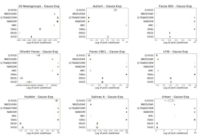
In figure 3, we show the performance of our algorithm and other competing baselines across our various datasets. Overall, we note that the best approximate posteriors are produced in the shortest time either by our Q-Transform algorithm or the Gibbs sampler for this model. Using random restarts for initialization yields approximate posteriors with similar Stein discrepancies to our approach but typically takes more time. The gradient-based approaches (even Q-SVGD which is initialized with Q-Transform) rarely do well, often plateauing at much higher discrepancies.
While the likelihood term in this model is invariant to (redundant) scalings8, a limitation is that the prior (chosen for computational convenience) is dependent on the scaling. We find that this is an undesirable feature because the posterior landscape includes infinite redundant scalings and therefore requires greater effort from the inference procedure to find appropriate scalings of factorizations. Another concern is that the likelihood model is not directly expressible in terms of whatever properties might be of interest to a practitioner. To address our concerns regarding the exponential-Gaussian model, we focus for the remainder of this work on the threshold-based model with scale-fixing prior.
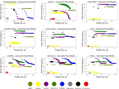
7.2. SILF-based Model Results
In figure 4, we show the performance of our algorithm and other competing baselines across our various datasets. Recall that the Stein discrepancy variational objective involves terms that consider both the quality of the factorizations (as given by the score function∇θlogp(θ) ) and their similarity (as given by the base RKHS kernelk(θi, θj)). The NNDSVDar
initial-izations and thinned HMC samples lead to factorinitial-izations that are high-quality but often not diverse (see diversity analysis in supplementary material: figures 24, 25, 26). The SVGD and the DSGD are generally the worst performing algorithms. These methods are often unable to find factorization parameters that meet the quality criteria of the SILF likelihood (see quality analysis in supplementary material: figures 18 and 19). This is understandable because even using simple gradient-based approaches to find a single high-quality NMF turns out to be difficult, hence the existence of a literature on specialized algorithms for performing NMF. Our Q-transform algorithm and random restarts are able to find
Stein discrepancy over time for exponential-Gaussian BNMF Discrete Posteriors
ples that are both high-quality and diverse, thus achieving the lowest Stein discrepancies; however, ourQ-transform algorithm does so in the shortest time.
Figures 31 and 32 in the Appendix show results for M ={25,50} where Q-Transform continues to have a runtime advantage over other baselines. Additionally, for some datasets (Olivetti Faces, LFW and Faces BIO) Q-Transform also produces higher quality of the posterior approximations. Variational posteriors constructed using thinned samples from HMC significantly lack diversity as the Stein discrepancies for collections of size 5, 25 and 50 are comparable. This indicates that the HMC chain only explores a small region of the posterior distribution and can be confirmed through the diversity analysis in the Appendix (figures 24, 25, 26). Sminchisescu et al. (2007) notes that in high dimensional spaces, we expect there to be many ridges of probability as there are likely to be some directions in which the posterior density decays sharply. Alternatively, there may be several isolated modes with no connecting regions of high probability making it particularly challenging for the HMC chain to avoid getting stuck in a local mode of the BNMF posterior.
Stein discrepancy over time for SILF BNMF Discrete Posteriors
Figure 5: The top 15 words for topic A (computers/electronics) and topic B (space) shows that different factorizations provide an emphasis on different terms. In topic A, the top word from factorization 1 and 2 is ‘card’, but it does not appear in the top 15 words of factorizations 3. Instead a similar term ‘chip’ is emphasized in Factorization 3. In topic B, the terms ‘space’ and ‘nasa’ appear in all three factorizations but factorization 2 is the only one with digital terms like ‘ftp’, ’server’,’site’ and ’faq’. In contrast factorization 1 and 3 both contain more physical terms like ‘sun’, ‘moon’,‘launch’.
7.2.1. Interpretation and Utilization of Posterior Estimates
BNMF posteriors can provide insight into the non-identifiability present within a particular dataset. Different factorizations may explain the data as a whole equally well, but do it through dictionary elements that have different interpretations, or can be used to understand specific parts of the data better than other factorizations. We show visual examples of diversity in the top words of the 20 Newsgroups BNMF posteriors and examples of how performance in downstream tasks for the 20 Newsgroups and Autism dataset is dependent on the posterior samples. Our analysis yields meaningful insights that could not be gained through a single factorization.
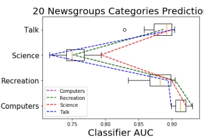
20-Newsgroups Our BNMF of 20-Newsgroups was a rank 16 decomposition of posts from 4 categories. In figure 6, we show the held-out AUC of a classifier trained to predict those categories based on the weights matrixW from each factorization in our variational posterior. Even though all of these factorizations have essentially equivalent reconstruction (see figure 19 in supplementary material), there exists a significant variation in the perfor-mance of these NMFs on the prediction tasks. The best performing NMF for one category is generally not the best (or even one of the top performing) NMFs for other categories. This observation may be valuable to a practitioner intending to use the NMF for some downstream task: different samples explain different patterns in the data. In figure 5, we see that this is indeed true: even after alignment,9 distinct NMF factorizations have top
words that indicate different emphasis across topics.
Autism Spectrum Disorder (ASD) In addition to core autism symptoms, Doshi-Velez et al. (2014) describe three major subtypes in autism spectrum disorder: those with higher rates of neurological disorder, those with higher rates of autoimmune disorders, and those with higher rates of psychiatric disorders. In figure 7, we show the number of topics that
Figure 6: Classifiers trained on feature vectors from different factorizations yield variability in prediction performance (as measured by AUC). The dotted lines show the factorization that produces the best performing classifier for each category. The factorization (blue dotted line) that predicts the ‘Talk’ category best is actually one of the worst performing factorizations for the ‘Science’ category. This variability in performance demonstrates that no single factorization gives the best latent representation for the overall prediction task.
contain key terms corresponding to these areas (expressive language disorder, epilepsy, asthma, and attention deficit disorder) across different factorizations in the variational pos-terior obtained viaQ-Transform. The large variation suggests that different factorizations in the particle-based posterior are spending different amount of modeling effort across these known factors; knowing that such uncertainty exists is essential for clinicians who may be trying to interpret topics to understand patterns in autism spectrum disorder.
On the same set of patients, we can also ask whether we can predict the onset of certain medical issues in the subsequent patient trajectory. We train a classifier on the weights of the NMFs to predict the onset of these medical issues. Similar to the category prediction results in 20-Newsgroups, figure 8 shows that there is a large variability (around 0.1 in AUC) in the performance of classifiers trained on the weights matrices of different factorizations on the prediction task. No single factorization has the best performance across the different prediction tasks.
7.3. Extension: BNMF in the presence of missing data
In the presence of missing data, there is perhaps an even greater need to understand the uncertainty in factorization parameters for NMF. The factorization space of a fully observed dataset forms a subset of the factorization space in the presence of missing data. Our particle-based approach to BNMF posterior approximation can be applied to the missing data setting by making some minor adjustments to the experimental settings.
The multiplicative update algorithm for NMF (Lee and Seung, 2001) can be adjusted so that the update equations for factorization parameters only consider the observed data. We use an implementation of this modification to the multiplicative update algorithm10to find a completion of the data X, compute the SVD subspace and then apply our Q-Transform initializations. Figure 9 demonstrates that our approach to BNMF can be extended to the
Figure 7: We explore top words in the topics relating to key terms of interest to clinicians and discover that different NMFs place varying amount of emphasis on different terms. Such variability is of interest to clinicians who may be trying to interpret topics to understand patterns in ASD.
Figure 8: Classifiers trained on weights matrix of Mmax = 100 different factorizations to
Figure 9: Under different percentages of missingness in the Olivetti Faces dataset (10%, 30%, 50%), the quality of the BNMF approximate posterior and the corresponding runtime ofQ-Transform and the other baselines is shown. The best discrete posterior approximations to BNMF are produced using the Q-Transform initializations (in red).
Figure 10: Sample factorizations from the variational posterior using Q-Transforms show that a diverse range of basis elements can be use to approximate the data. However, HMC samples seem to be identical indicating that HMC was only exploring a very small region of the posterior space.
case where the data matrix X is partially observed. For the Olivetti Faces dataset with varying degrees of missingness, the Q-Transform approach to BNMF consistently finds posterior approximations that are significantly better (as measured by Stein discrepancy) than other baselines whereas for a given M, the runtime is second-lowest.
from HMC have basis elements that look identical. This indicates that the HMC has explored a limited region of the posterior space.
8. Discussion: When is Q-Transform successful?
Our ability to extract transferable low-rank transformation matrices from an SVD and an instance of NMF indicates that there exist similarities across different NMF problems. In this Section we seek to develop a better intuition behind the success of the Q-Transform initializations at exploiting these similarities. In this Section, we provide discussion and smaller-scale experiments to shed light on when, why, and how our Q-transform approach is successful.
8.1. Q-Transform Generating Process
In our approach, we generated candidate Q-Transform matrices (Algorithm 2) by applying random restarts to small, synthetic data sets. We focused on this approach because small datasets are much faster to train, and with synthetic data sets, we can know at least one ground truth NMF and level of noise. However, there are obviously a large number of choices for the data used to generate candidateQ-Transform matrices.
In figure 11, we present results with a variety of different methods for generating candi-dates. In all cases, the source data was of small dimension (XS ∈R15×15), and the target
data was larger (XT ∈ R500×500). The target data had a true non-negative rank of 10
and factors were generated with i.i.d. entries from a standard normal. In all these experi-ments we set the transfer rank to be RT =RSVD = 3. We explored six ways of generating
candidates from the source data:
• Uniform data: Generating a dataset XS where each entry is i.i.d. with a uniform
distribution in [0,1]; then apply random restarts to find candidate transforms.
• Simple sub-sample data: Generating dataset XS by uniformly selecting 15 rows and
columns of the target dataXT; then apply random restarts to find candidate
trans-forms
• Column-projection data: Generating dataset XS by sub-sampling 15 columns of XT
and applying a random projection intoR15 for each each column; then apply random
restarts to find candidate transforms.
• Dirichlet factors: Generating factorsA,W with each column ofA, W from a Dirichlet distribution (with concentration parameterαset to 1); letXS =AW+Gaussian Noise;
then apply random restarts to find candidate transforms.
• Uniform factors: Generating factors A, W with each entry i.i.d. from a uniform distribution in [0,1]; let XS =AW + Gaussian Noise; then apply random restarts to
find candidate transforms.
• Gaussian factors: Generating factors A, W with each entry i.i.d. from a standard normal distribution; let XS =AW+ Gaussian Noise; then apply random restarts to
The methods that produced the source data from some true NMF factors produced candi-date transformations that resulted in the highest quality initializations on the target data (figure 11). In settings where a practitioner deals with a collection of similar NMF datasets (e.g. music analysis, hyper spectral images), there may be more clever ways in which the NMF solution spaces corresponding to a real dataset may yield more appropriate Q -Transforms specific to that type of data. Finally, we find in figure 12 that the performance of Gaussian factors method does not vary with the rank of the synthetic data (the transfer rank is still held fixed).
Figure 11: For different synthetic data XS
generating procedures, we show the initial-ization quality obtained via the Q-Transform matrices on a target data XT. Dirichlet,
Uniform, Gaussian have significantly supe-rior performance compared to Sub-sample, Column-projection and Uniform data. For comparison, we show the quality of NMF so-lutions (solid line) and random initializations (dashed line).
Figure 12: Using Gaussian factors for the synthetic data generation process with different ranks does not appear to change the quality of the Q-Transform initialization qual-ity on the target data XT. This
in-dicates that this generating proce-dure is not sensitive to the rank in order to produce high quality (close to true NMF solution) initializations usingQ-Transform. For comparison, we show the quality of NMF solu-tions (solid line) and random initial-izations (dashed line).
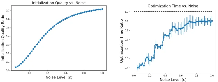
8.2. The Q-Transform Initialization versus Noise
In Section 4, we sought high-quality initializations because they generally require less time to converge. On synthetic target dataXT =AW+No (D = N = 500, R = 20) we explore
the effect of increasing noise () on the quality of our transfer-based NMF initializations and the time taken to converge. Specifically: are there noise regimes in which the Q-transform method works better, and noise regimes in which it does not?
We normalize the norm of the noise matrix to be equal to the norm of the datakNok= kAWk so that the contribution of signal AW and noise No to the data is equal when
= 1. We continue to use the same 100 pairs of QA, QW matrices. We compare the
Figure 13: In the low-noise regime, the reconstruction error of Q-Transform initializations is significantly less than random restart initializations. This relative advantage gets smaller as the noise level increases. Similarly, the time taken to converge is significantly shorter than the random restart approach under the low noise scenario and continues to increase with noise. As expected, at high noise levels there exists no additional advantage to the
Q-Transform approach (the optimization time ratio approaches 1).
and time to convergence (ratio of time taken usingQ-Transform initialization to time taken using random restart). In both metrics, the Q-Transform has an advantage over random restarts for values of the noise smaller than 1, and the advantage is greatest for smallest noise. Figure 13 shows that the advantage ofQ-Transform initializations is highest in a low noise regime and decreases as the noise increases. This behavior makes sense because as noise increases, the data is no longer truly low rank.
8.3. Selecting ranks
We emphasize that there are two distinct ranks that need to be chosen when applying our technique. The first is the rank of the factorizationRNMF. There exist multiple approaches
for choosing this rank, e.g. Tan and F´evotte (2009); Alquier and Guedj (2017), and they can be applied to our approach (as well as any other NMF algorithm).
The second is choosing the transfer rank RT. The transformation dimensions RT and
RSVDdetermine the dimensions of transformation matricesQA, QW which map basis vectors
defining the top SVD subspace of dimensionRSVDto a set ofRT non-negative basis vectors
that approximate the same subspace. The full initialization for NMF is obtained by either padding the initialization with small entries (RT < RNMF) or removing extra columns and
rows of the factor matrices (RT > RNMF). (For simplicity, we consider the case where
the transfer rank and SVD rank are equal RT = RSVD and the resulting transformation
matrices QA, QW are square.)
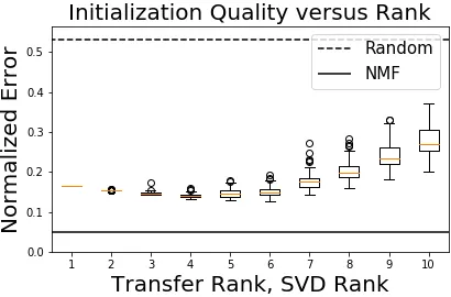
The choice of the transfer rank RT is specific to our algorithm, and in figure 14 we
investigate how well our transfer learning performs for different choices of transfer rankRT.
In the experiment, we extract a set of 100 transformation matrices QA, QW for transfer
dimensions RT =RSVD ={1,2, . . . ,10} using synthetic source data (D=N = 15). Once
constructed, we applied the transformation matrices to a 500×500 target datasetXT of rank
Figure 14: On a synthetic target dataset (D = N = 500, KNMF = 10), we apply Q
-Transform initializations using varying transfer ranks and SVD ranks RT = RSVD = {1,2, . . . ,10}. We see that for a range of low rank values, the Q-Transform initializa-tions are high quality, but at larger values the quality of initializainitializa-tions gets worse. The dotted line shows the quality of random initializations and the solid line shows the quality NMF solutions. The reconstruction errors are normalized by the norm of the data.
matrices found using the 15×15 synthetic source dataset are unable to successfully transfer to this new dataset. We see that the error initially decreases, but then increases as the transfer rank increases. This result suggests that the top directions of variation hold the most transferable information across NMF problems.
8.4. Sign Convention for SVD
In considering whenQ-Transform is successful, we note that there exists an intrinsic ambi-guity in the sign of the singular vectors ofX: changing the sign of any column ofASVD and
corresponding row ofWSVD gives a valid SVD. ForQ-Transform to work, we must apply a
consistent resolution of the sign ambiguity (e.g. from Bro et al. (2008)). This ensures that learned transformations QA, QW map in a consistent way to SVD decompositions of new
datasets.
9. Related Work
Closer to the goals of our work, Gershman et al. (2012) develop a non-parametric ap-proach to variational inference that provides flexibility in modeling the number of Gaussian components required to approximate a posterior. However, the isotropic covariance in the model makes it unsuitable for applying it to BNMF. With regard to the inference pro-cess, ourQ-Transform approach to finding multiple optima is most similar to Roˇckov´a and George (2016) and Paatero and Tapper (1994), who use rotations to find solutions to a sin-gle matrix factorization problem that are sparse and non-negative respectively. In contrast, we use rotations to find multiple non-negative solutions, and also demonstrate how these rotations can be re-used for transfer learning.
More broadly, recent work on NMF has involved theoretical work on non-identifiability with new algorithms that can provably recover the NMF under certain assumptions (Li and Liang, 2017; Bhattacharya et al., 2016; Ge and Zou, 2015a). However, these assumptions are often difficult to check and may indeed be violated in practice; Bayesian methods typically provide more flexibility in modeling and assumptions.
All of the works above typically assume some desired factorization rank. There also exists work on models that automatically detect the rank—through automatic relevance determination for NMF (Tan and F´evotte, 2009) or more recently, via a rank-adaptive prior Alquier and Guedj (2017). These works are complementary to ours, in that those techniques could be combined with our transfer-based approach of generating candidates of whatever rank those algorithms determine is appropriate.
The ability of Stein discrepancies to assess the quality of any collection of particles (Gorham and Mackey, 2015) has resulted in large recent interest in other ways to create collections of samples (Oates et al., 2017; Liu and Wang, 2016). Liu et al. (2016) and Chwialkowski et al. (2016) showed that kernelized Stein discrepancy could be computed analytically in Reproducing Kernel Hilbert Spaces (RKHS); Pu et al. (2017) and Feng et al. (2017) use neural networks instead. Ranganath et al. (2016) establish the Stein discrepancy as a valid variational objective. To our knowledge, Stein discrepancy-based posterior approximation has not been applied to NMF, and yet, we see that it allows us to leverage existing non-Bayesian approaches to characterize these multi-modal posteriors. In our work, the Dirichlet prior on the columns of the basis matrix A is important to ensure that we avoid a known saddle point of the zero factorization (from likelihood term) that yields a corresponding zero for the score function.
10. Conclusion
In this work, we presented a novel transfer learning-based approach to posterior estima-tion in BNMF. Simply creating collecestima-tions of factorizaestima-tions via random restarts on our
Through Q-Transform, we introduce a way to speed-up the process of finding multiple diverse NMFs. The discovery that Q-Transform matrices can transfer from synthetic to multiple real datasets is exciting and also suggests interesting questions for further research. For example, what is the theoretical nature of the similarities between principal eigenspaces of different non-negative matrices and the relation between their SVD and NMF bases? And, how does the synthetic data generation process used to obtainQ-Transform matrices impact the initializations and the effectiveness of the Q-Transform algorithm in general?
More broadly, our qualitative results demonstrate that even relatively simple models, such as NMF, can have multiple optima that are comparable under the objective function but have large variation in how well they explain different portions of the data—or how they perform on different downstream tasks. Thus, it is important to be able to compute these posteriors efficiently.
Acknowledgments
References
20NG. The 20 newsgroups text dataset scikit-learn 0.19.1 documentation. http:// scikit-learn.org/stable/datasets/twenty_newsgroups.html, July 2013. (Accessed on 01/23/2018).
Pierre Alquier and Benjamin Guedj. An oracle inequality for quasi-Bayesian Nonnegative Matrix Factorization. Mathematical Methods of Statistics, 26(1):55–67, 2017.
Yoann Altmann, Nicolas Dobigeon, and Jean-Yves Tourneret. Unsupervised post-nonlinear unmixing of hyperspectral images using a Hamiltonian Monte Carlo algorithm. IEEE Transactions on Image Processing, 23(6):2663–2675, 2014.
Morten Arngren, Mikkel N Schmidt, and Jan Larsen. Unmixing of hyperspectral images using Bayesian Non-Negative Matrix Factorization with volume prior. Journal of Signal Processing Systems, 65(3):479–496, 2011.
Sanjeev Arora, Rong Ge, Ravindran Kannan, and Ankur Moitra. Computing a Non-Negative Matrix Factorization–provably. In Proceedings of the forty-fourth annual ACM symposium on Theory of computing, pages 145–162. ACM, 2012.
Andrew D Barbour and Timothy C Brown. Stein’s method and point process approxima-tion. Stochastic Processes and their Applications, 43(1):9–31, 1992.
Atilim Gunes Baydin, Barak A Pearlmutter, Alexey Andreyevich Radul, and Jeffrey Mark Siskind. Automatic differentiation in machine learning: a survey. arXiv preprint arXiv:1502.05767, 2015.
Nancy Bertin, Roland Badeau, and Emmanuel Vincent. Fast Bayesian NMF algorithms enforcing harmonicity and temporal continuity in polyphonic music transcription. In
Applications of Signal Processing to Audio and Acoustics, 2009. WASPAA’09. IEEE Workshop on, pages 29–32. IEEE, 2009.
Michael Betancourt. Cruising the simplex: Hamiltonian Monte Carlo and the Dirichlet distribution. In AIP Conference Proceedings 31st, volume 1443, pages 157–164. AIP, 2012.
Chiranjib Bhattacharya, Navin Goyal, Ravindran Kannan, and Jagdeep Pani. Non-Negative Matrix Factorization under Heavy Noise. InInternational Conference on Machine Learn-ing, pages 1426–1434, 2016.
Chiranjib Bhattacharyya, IISC ERNET, Navin Goyal, COM Ravindran Kannan, and COM Jagdeep Pani. Non-Negative Matrix Factorization under heavy noise. In Pro-ceedings of The 33rd International Conference on Machine Learning, pages 1426–1434, 2016.
Christos Boutsidis and Efstratios Gallopoulos. SVD based initialization: A head start for Non-Negative Matrix Factorization. Pattern Recognition, 41(4):1350–1362, 2008.
Rasmus Bro, Evrim Acar, and Tamara G Kolda. Resolving the sign ambiguity in the Singular Value Decomposition. Journal of Chemometrics, 22(2):135–140, 2008.
Jean-Philippe Brunet, Pablo Tamayo, Todd R Golub, and Jill P Mesirov. Metagenes and molecular pattern discovery using Matrix Factorization. PNAS, 101(12):4164–4169, 2004.
CBCL. Home — poggio lab. http://poggio-lab.mit.edu/, 2000. (Accessed on 01/23/2018).
Ali Taylan Cemgil. Bayesian inference for Non-Negative Matrix factorisation models. Com-putational Intelligence and Neuroscience, 2009, 2009.
Wei Chu, S Sathiya Keerthi, and Chong Jin Ong. Bayesian support vector regression using a unified loss function. IEEE transactions on neural networks, 15(1):29–44, 2004.
Kacper Chwialkowski, Heiko Strathmann, and Arthur Gretton. A kernel test of goodness of fit. arXiv preprint arXiv:1602.02964, 2016.
Andrzej Cichocki and Anh-Huy Phan. Fast local algorithms for large scale Non-Negative Matrix and Tensor Factorizations. IEICE transactions on fundamentals of electronics, communications and computer sciences, 92(3):708–721, 2009.
Steven Diamond and Stephen Boyd. Cvxpy: A python-embedded modeling language for convex optimization. The Journal of Machine Learning Research, 17(1):2909–2913, 2016.
Onur Dikmen and A Taylan Cemgil. Unsupervised single-channel source separation us-ing Bayesian NMF. In Applications of Signal Processing to Audio and Acoustics, 2009. WASPAA’09. IEEE Workshop on, pages 93–96. IEEE, 2009.
David Donoho and Victoria Stodden. When does Non-Negative Matrix Factorization give a correct decomposition into parts? InAdvances in neural information processing systems, page None, 2003.
Finale Doshi-Velez, Yaorong Ge, and Isaac Kohane. Comorbidity clusters in autism spec-trum disorders: an electronic health record time-series analysis. Pediatrics, 133(1):e54– e63, 2014.
Yihao Feng, Dilin Wang, and Qiang Liu. Learning to draw samples with amortized Stein Variational Gradient Descent. arXiv preprint arXiv:1707.06626, 2017.
C´edric F´evotte and J´erˆome Idier. Algorithms for Non-Negative Matrix Factorization with the β-divergence. Neural computation, 23(9):2421–2456, 2011.