Attitude towards E-learning Technology -- A study in Kerala

(1)

Volume-5, Issue-1, February-2015

International Journal of Engineering and Management Research

Page Number: 308-313

Block Matching and 3D Filtering for Image Denoising

Abhinit Bajaj1, Sukhjit Singh2 1

M.Tech (Student), ECE Section, GTBKIET Chhapianwali, Malout, INDIA 2

Assistant Professor, ECE Section, GTBKIET Chhapianwali, Malout, INDIA Punjab Technical University, Jalandher, INDIA

ABSTRACT

We present a novel approach to still image denoising based on effective filtering in 3D transform domain by combining sliding-window transform processing with block-matching. We process blocks within the image in a sliding manner and utilize the block-matching concept by searching for blocks which are similar to the currently processed one. The matched blocks are stacked together to form a 3D array and due to the similarity between them, the data in the array exhibit high level of correlation. We exploit this correlation by applying a 3D decorrelating unitary transform and effectively attenuate the no1ise by shrinkage of the transform coefficients. The subsequent inverse 3D transform yields estimates of all matched blocks. After repeating this procedure for all image blocks in sliding manner, the final estimate is computed as weighed average of all overlapping block estimates.

A fast and efficient algorithm implementing the proposed approach is developed. The experimental results show that the proposed method delivers state-of-art denoising performance, both in terms of objective criteria and visual quality.

Keywords: Image Denoising, Block-matching, 3D transforms.

I. INTRODUCTION

In these methods we undertake the block-matching concept for a single noisy image; as we process image blocks in a sliding manner, we search for blocks that exhibit similarity to the currently-processed one. The matched blocks are stacked together to form a 3D array. In this manner, we induce high correlation along the dimension of the array in which the blocks are stacked. We exploit this correlation by applying a 3D decorrelating unitary transform which produces a sparse representation of the true signal in 3D transform domain. Efficient noise attenuation is done by applying a shrinkage operator (e.g. hard thresholding or Wiener filtering) on the transform coefficients. This results in improved denoising performance and effective detail preservation in the local estimates of the matched blocks, which are reconstructed by an inverse 3D transform of the filtered coeffcients. After

processing all blocks, the final estimate is the weighted average of all overlapping local block-estimates. Because of overcompleteness which is due to the overlap, we avoid blocking artifacts and further improve the estimation ability.

II. DENOISING BY SHRINKAGE

IN 3D TRANSFORM DOMAIN WITH

BLOCK-MATCHING

Let us introduce the observation model and notation used throughout the chapter. We consider noisy observations z : X→ R of the form

z (x) = y (x) + η (x), where x

∈

X is a 2D spatial coordinate that belongs to the image domain X , y is the true image, and η (x) is white Gaussian noise of zero mean and variance

σ

2. By

Z

_x we denote a block of fixed size N1

×N1

x

Z

extracted from z, which has z (x) as its upper-left element; alternatively, we say that is located at x. With

y

ˆ

we designate the final estimate of the true image.

A- Local Estimates

We successively process all overlapping blocks of fixed size in a sliding manner, where "process" stands for the consecutive application of block-matching and denoising in local 3D transform domain. For the sub-subsections to follow, we fix the currently processed block as

Z

xR, where

x

R

∈

X

, and denominate it as "reference block".

B- Block-matching

(2)

similarity) as

( )

(

,

2 log(

)

||

)

,

(

Z

₁

Z

₂

N

₁1

T

₂

Z

₁ ₂

N

₁2

d

_x _x

=

−

γ

_D _x

λ

_thr _D

σ

(

)

2

)

₂

1 2

2

2 Z , 2log(N ) ||

T D x

λ

thr D

σ

γ

− (1)

where x1, x2

∈

X,

T

₂_D is a 2D linear unitary transform

operator (e.g. DFT),

γ

is a hard-threshold operator,

D thr2

λ

is fixed threshold parameter, and || ||2 denotes the

L2 - norm. Naturally,

γ

is defined as













>

=

otherwise

if

thr thr

,

0 |

|

,

)

,

(

λ

γ

The result of the block-matching is a set

S

_xR

⊆

X

of the coordinates of the blocks that are similar to

Z

_xR according to our d-distance (1); thus, SxR

},

)

,

(

|

{

xR x match

xR

x

X

d

Z

S

=

∈

<

τ

is defined as

(2)

where

τ

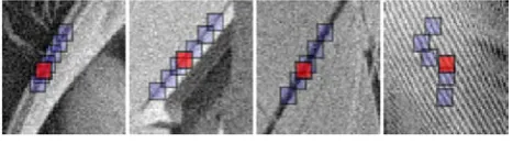
_match is the maximum d-distance for which two blocks are considered similar. The matching procedure in presence of noise is demonstrated on Figure 1, where we show a few reference blocks and the ones matched as similar to them.

Figure 1 Fragments of Lena, House, Boats and

Barbaracorrupted by AWGN of σ = 15. For each fragment

block matching is illustrated by showing a reference block marked shown with red color and a few of its matched ones.

C- Denoising in 3D transform domain

We stack the matched noisy blocks

Z

_x_∈_SxR

(ordering them by increasing d-distance to

Z

_xR) to form a 3D array of size N1 × N1 × |SxR|, which is denoted by ZSxR . We apply a unitary 3D transform T3D on ZSxR

1 3

−

D

T

in order to attain sparse representation of the true signal. The noise is attenuated by hard-thresholding the transform coefficients . Subsequently, the inverse transform operator yields a 3D array of reconstructed estimates

ˆ

SxR

=

T

₃D1

(

γ

(

T

₃D

(

SxR

)

,

λ

thr₃D

σ

2 log

( )

N

₁2

)

−

Z

Y

(3)

where λthr3D is a fixed threshold parameter. The array

Y

ˆ

_SxR

comprises of |SxR

xR SxR x

Y

ˆ

_∈ | stacked local block estimates of

the true image blocks located at x

∈

S

_xR. We define a weight for these local estimates as

















_≥

=

otherwise

N

if

N

w

har har xR

,

1

1 ,

1

(4)

where Nhar

xR SxR x

Y

ˆ

_∈

is the number of non-zero transform coefficients after hard-thresholding.

D- Estimate Aggregation

After processing all reference blocks, we have a set of local block estimates (and their corresponding weights wxR

y

ˆ

), which constitute an overcomplete representation of the estimated image due to the overlap between the blocks. The final estimate is computed as a weighted average of all local ones as given by

∑

∈ ∈ ∈ ∈

=

SxR

xm xR xm

X xR SxR xm xR xm xR X xR

x

w

x

Y

w

x

y

)

(

)

(

ˆ

)

(

ˆ

χ

(5)

where

χ

_xm is the characteristic function of the square support of a block located at xm

R

:

X

→

e

.

III. WIENER FILTER EXTENSION

Provided that an estimate of the true image is available (e.g. it can be obtained from the method given in the previous section), we can construct an empirical Wiener filter as a natural extension of the above thresholding technique. Because it follows the same approach, we only give the few fundamental modifications that are required for its development and thus omitting repetition of the concept. Let us denote the initial image estimate by . In accordance with our established notation,

Ex

∈

designates a square block of fixed size N1 × N1, extracted from e and located at x X.

A- Modification to Block-Matching

In order to improve the accuracy of block-matching, it is performed within the initial estimate e rather than the noisy image. Accordingly, we replace the thresholding based d-distance measure from (1) with the normalized L2-norm of the difference of two blocks with subtracted means. Hence, SxR

(

) (

)

{

xR xR x x match

}

xR

x

X

N

E

S

=

∈

|

₁−1

||

−

||

₂

<

τ

becomes

(6)

where

E

_xR and

E

_xare the mean values of the blocks ExR

and Ex, respectively. The mean subtraction allows for

(3)

The linear Wiener filter replaces the nonlinear hard-thresholding operator. The attenuating coefficients for the Wiener filter are computed in 3D transform domain as

₂ ₂

3

2 3

|

)

(

|

)

(

|

σ

+

=

SxR D

SxR D SxR

T

E

W

,

where ESxR is a 3D array built by stacking the matched blocks. We filter the 3D array of noisy observations ZSxR in

T3D-transform domain by an elementwise multiplication

with WSxR.

(

)

(

SxR D SxR

)

D

SxR

T

W

T

Z

Y

ˆ

=

₃−1 ₃

The subsequent inverse transform gives

, (7)

where

Y

ˆ

_SxR comprises of stacked local block estimates of the true image blocks located at the matched locations. As in (4), the weight assigned to the estimates is defined as

1 |

|

1

2 1

1 1

1

|

)

,

(

|

−

= =

=













=

∑

SxR t

SxR N

j N

i

xR

i

j

t

w

W

(8)

IV. ALGORITHM

We present an algorithm which employs the hard-thresholding approach to deliver an initial estimate for the Wiener filtering part that produces the final estimate. A straightforward implementation of this general approach is computationally demanding. Thus, in order to realize a practical and efficient algorithm, we impose constraints and exploit certain expedients.

It is often assumed that neighboring pixels in small blocks extracted from natural images exhibit high correlation; thus, such blocks can be sparsely represented by well-established decorrelating transforms, such as the DCT, the DFT, wavelets, etc. From computational efficiency point of view, however, very important characteristics are the separability and the availability of fast algorithms. Hence, the most natural choice for T2D and

T3D

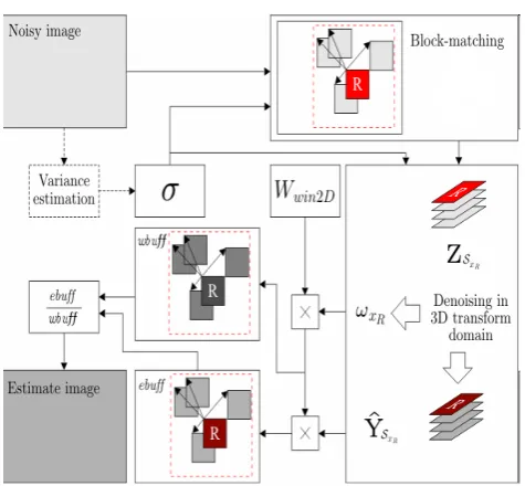
Figure 2 Flowchart for denoising by hard-thresholding in 3D transform domain with block-matching .

blocks by setting an integer N

is a fast separable transform which allows for sparse representation of the true-image signal in each dimension of the input array.

Efficient Image Denoising Algorithm with Block-Matching and 3D Filtering

Let us introduce constraints for the complexity of the algorithm. First, we fix the maximum number of matched

2 to be the upper

bound for the cardinality of the sets SxR. Second, we do

block-matching within a local neighbourhood of fixed size

NS × NS cantered about each reference block, instead of

doing it in the whole image. Finally, we use Nstep as a step

by which we slide to every next reference block. Accordingly, we introduce XR

⊆

X as the set of the

reference blocks’ coordinates, where

|

₂

|

step R

N

X

≈

In order to reduce the impact of artifacts on the borders of blocks (border effects), we use a Kaiser window

Wwin2D (with a single parameter β) as part of the weights of

the local estimates. These artifacts are inherent of many transforms (e.g. DFT) in presence of sharp intensity differences across the borders of a block.

Let the input noisy image be of size M ×N, thus |X| = MN. We use two buffers of the same size, ebuff for estimates and wbuff for weights to represent the summations in the numerator and denominator, respectively, in (5.5). For simplicity, we extend our notation so that ebuff(x) denotes a single pixel at coordinate x and

ebuffx

∈

designates a block located at x in ebuff (the same notation is to be used for wbuff ). A flowchart of the hard-thresholding part of the algorithm is given in Figure 2 (but we do not give such for the Wiener filtering part since it requires only the few changes.). Following are the steps of the image denoising algorithm with block-matching and 3D filtering.

(i).Initialization. Initialize ebuff (x) = 0 and wbuff (x) = 0, for all x X.

(ii). Local hard-thresholding estimates. For each xR

∈

(4)

(2) but restrict the search to a local neighbourhood of fixed size NS ×NS centred about xR. If |SxR| >

N2, then let only the coordinates of the N2 blocks

with smallest d-distance to ZxRremain in SxR

xR SxR x

Y

ˆ

_∈

and exclude the others.

(b) Denoising by hard-thresholding in local 3D transform domain. Compute the local estimate blocks and their corresponding weight wxR

xR x

Y

ˆ

as given in (3) and (5.4), respectively.

(c) Aggregation. Scale each reconstructed local block estimate , by a block of weights W(xR) = wxR

Wwin2D and accumulate to the estimate buffer:

ebuffx=ebuffx + W(xR

xR x

Y

ˆ

) , for all x

∈

SxR.

Accordingly, the weight block is accumulated to

same locations as the estimates but in the

weights buffer: wbuffx=wbuffx + W(xR

∈

SxR ) , for all x

)

(

)

(

)

(

x

wbuff

x

ebuff

x

e

=

.

(iii). Intermediate estimate. Produce the intermediate

estimate( for all x

∈

X, which is to be

used as initial estimate for the Wiener counterpart.

(iv). Local Wiener filtering estimates. Use e as initial estimate. The buffers are re-initialized: ebuff (x) = 0 and

wbuff (x) = 0, for all x

∈

X. For each xR

∈

XR, do the

following sub-steps.

(a) Block-matching. Compute SxR as given in (6) but

restrict the search to a local neighbourhood of fixed size NS ×NS cantered about xR. If |SxR| > N2,

then let only the coordinates of the N2 blocks with

smallest distance to ExR remain in SxR

xR SxR x

Y

ˆ

_∈

and exclude the others.

(b) Denoising by Wiener filtering in local 3D transform domain. The local block estimates and their weight wxR

)

(

)

(

)

(

ˆ

x

wbuff

x

ebuff

x

y

=

are computed as given in (7) and (8), respectively.

(c) Aggregation. It is identical to step (ii)c.

(v). Final estimate. The final estimate is given by

, for all x

∈

X.

V. RESULTS AND DISCUSSION

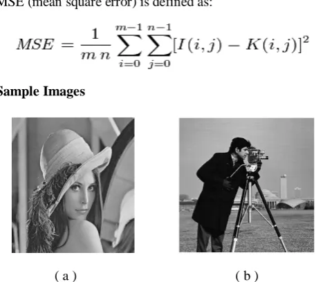
We present experiments conducted with the algorithm introduced in Section 4, where the transforms T2D and T3D are the 2D DFT and the 3D DFT, respectively. All results are produced with the same fixed parameters–but different for the hard-thresholding and Wiener filtering parts. We consider two sample images

Lena(512x512 pixels) and Cameraman (256x256 pixels) as shown below for proposed method ,SADCT[] and K-SVD[]. We summarize the results of the proposed technique in terms of output peak signal-to-noise ratio (PSNR) in decibels (dB), in table1 and table2 for Lena and Cameraman image respectfully. The diagrams below also shows their respective graphs and reconstructed images This is used to compare the relative filtering performance of various methods. The PSNR between the filtered output image K(i,j) and the original image I(i,j) of dimension M × N pixels is defined as:

Here, MAXI is the maximum possible pixel value of the image. When the pixels are represented using 8 bits per sample, this

Sample Images

MSE (mean square error) is defined as:

( a ) ( b )

Figure 3: Sample images considered ( a ) Lena image , ( b ) Cameraman image

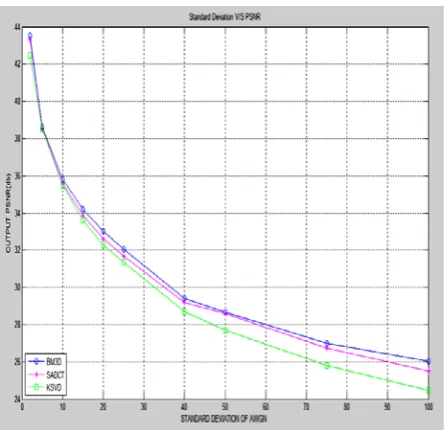
PSNR values for Lena Image

METHODS→ BM3D-DFT

SA-DCT

K-SVD ↓

STANDARD DEVIATION

OF GAUSSIAN

NOISE

2 43.52 43.33 42.46

5 38.63 38.54 38.52

10 35.82 35.58 35.47

15 34.21 33.86 33.6

20 33.03 32.62 32.28

25 32.06 31.66 31.33

40 29.41 29.17 28.7

50 28.68 28.59 27.69

75 27.01 26.75 25.8

(5)

standard deviation of AWGN of noisy image for BM3DFT,SADCT and KSVD.

Graphs for Lena Images

Graph 1 : PSNR Values for denoised image versus standard deviation of AWGN for Lena image for BM3DFT,SADCT and KSVD

Reconstructed Images For Lena

(a) (b)

( c ) ( d )

Figure 4: Lena images ( a ) noisy image with standard deviation of AWGN 20 , denoised images with ( b ) KSVD ( c ) SADCT ( d ) BM3DFT.

PSNR values for Cameraman Image

METHODS→

BM3D-DFT

SA-DCT K-SVD ↓

STANDARD DEVIATION

OF GAUSSIAN

NOISE

2 _43.74 _43.54 _43.14 5 37.99 37.15 37.01

10 _33.76 _33.98 _32.08 15 31.5 31.7 31.52

20 30.34 30.18 30.02

25 29.08 29.11 28.79

40 26.97 26.9 26.16

50 25.55 25.38 25.12

75 24.29 23.87 23.62

100 22.73 22.49 22.32

Table 2: PSNR Values for denoised Cameraman image versus standard deviation of AWGN of noisy image for BM3DFT,SADCT and KSVD.

Graphs for Cameraman Image

Graph 2 : PSNR Values for denoised image versus standard deviation of AWGN for Cameraman image for BM3DFT, SADCT and KSVD

Reconstructed Images for Cameraman

(6)

( c ) ( d )

Figure 5: Cameraman images ( a) noisy image with standard deviation of AWGN 20 , denoised images with ( b ) KSVD ( c ) SADCT ( d ) BM3DFT

We conclude by remarking that the proposed method outperforms–in terms of objective criteria–all techniques known to us. Moreover, our estimates retain good visual quality even for relatively high levels of noise.

Our current research extends the presented approach by the adoption of variable-sized blocks and shapeadaptive transforms, thus further improving the adaptivity to the structures of the underlying image. Also,application of the technique to more general restoration problems is being considered.

REFERENCES

[1] M. J.Wainwright and E. P. Simoncelli, “Scale mixtures of Gaussians and the statistics of natural images,” in Adv. Neural Information Processing Systems, S. A. Solla, T. K. Leen, and K. R. Müller, Eds. Cambridge, MA: MIT Press, 2000, vol. 12, pp. 855–861.

[2] L. Yaroslavsky, K. Egiazarian, and J. Astola, "Transform domain image restoration methods: review, comparison and interpretation," in Nonlinear Image Processing and Pattern Analysis XII, Proc. SPIE 4304,pp. 155—169, 2001.

[3] V. Katkovnik, K. Egiazarian, and J. Astola, “Adaptive window size image de-noising based on intersection of confidence intervals (ICI) rule,” Math. Imag. Vis., vol. 16, no. 3, pp. 223–235, May 2002.

[4] Rafael C. Gonzalez and Richard E. wood,Steven L. Eddins,” Digital Image Processing Using MATLAB”,Pearson education, 2006.

[5] A. Foi, K. Dabov, V. Katkovnik, and K. Egiazarian, "Shape-Adaptive DCT for Denoising and Image Reconstruction," in Electronic Imaging’06, Proc. SPIE 6064, no. 6064A-18, San Jose, California USA, 2006 [6] Eero P. Simoncelli ,Edward H. Adelson “Noise removal via bayesian wavelet coring” Proceedings of IEEE International Conference on Image Processing. Vol. 14, pp. 379-382. Lausanne, Switzerland. 2009

[7] Lei Zhang, weisheng Dong, David Zhang, Guangming Shi,” Two-stage image denoising by principal component analysis with local pixel grouping.”Science Direct Journal on Pattern Recognition, volume 43, issue 4, April 2010, Pages 1531-1549.

[8] J. Portilla, V. Strela, M. Wainwright, and E. P. Simoncelli,”Image denoising using a scale mixture of

Gaussians in the wavelet domain”. IEEE Trans. Image Process., vol. 12, no. 11,pp. 1338.1351, November 2010. [9] M. Elad and M. Aharon, “Image denoising via sparse and redundant representations over learned dictionaries”.

IEEE Trans. on Image Process., vol. 15, no. 12, pp. 3736.3745, December 2011...

[10] A. Buades, B. Coll, AND J. M. Morel “A review of image denoising algorithms, with a new One” MULTISCALE MODEL. SIMUL. c_ 2012 Society for Industrial and Applied Mathematics, Vol. 4, No. 2, pp. 490–530

[11]C. A. Graves “Deblocking of dct-compressed images using noise injection Followed by image denoising” Proceedings of the International Conference on Information Technology: Computers and Communications © 2013 IEEE