MURDOCH RESEARCH REPOSITORY
http://dx.doi.org/10.1109/IJCNN.1992.227189
Morrison, M. and Attikiouzel, Y. (1992) A probabilistic neural
network based image segmentation network for magnetic
resonance images. In: International Joint Conference on Neural
Networks, IJCNN 92, 7 - 11 July, Baltimore, MD, USA,
pp. 60 – 65 Vol 3.
http://researchrepository.murdoch.edu.au/20249/
Copyright © 1992 IEEE
Personal use of this material is permitted. However, permission to reprint/republish
this material for advertising or promotional purposes or for creating new collective
A Probabilistic Neural Network Based Image Segmentation
Network
for
Magnetic Resonance Images
M.Monison and
Y.
Attikiouzel
Centre for Intelligent Information Processing Systems
University of Western Australia.
Abstract
A network structure for segmenting magnetic resonance medical images is proposed. The network incorporates
a
probabilistic neural network to facilitate the generationof
likelihood estimates for use in an iterative segmentation process, which is shown to produce good segmentation results on real MRI images.1.
Introduction
Magnetic resonance imaging (MRI) is an extremely powerful tool for use in the visualisation of two- dimensional cross-sectional images of Uie internal structure of the human body. Whilst still in its infancy as a diagnostic imaging modality, MRI is gaining ever increasing acceptance as a safe, non-invasive companion to the more common technique of x-ray CT (or CAT scan),
MRI is a relatively high resolution imaging teclinology and as such, is ideally suited to the task of volumetric tissue analysis. Such analysis can be extremely valuable as an aid in the treatment of muscle wasting diseases or in the assessment of muscle development programs for sportsmen. Unfortunately, in order to calculate the desired tissue volume, the region of interest (ROI) must be identified and isolated in every cross-sectional image containing the ROI, which, for a high resolution image, may be in the vicinity of one hundred images or more. In addition, not only must the ROI be identified in every image, but each image must then be painstakingly segmented using a mouse or similar pointing device, in order to isolate the desired tissue for the volumetric calculations. An automated MRI image segmentation system is UIUS of critical importance in the development of any practical volumetric analysis system.
Current research into image segmentation (see [l] for a recent review) has tended to produce algorithms which rely 011 a high degree of a-priori morphological and/or physical consistency information typically manifested in tlie form of complex rule-based systems. This approach has the drawback that not only is the processing of such information computationally expensive but it is also extremely difficult to encode in any robust and situationally invariant manner.
At the olher end of the spectrum, simple, single-pass segmentation algorithms incorporating a minimum of prior knowledge are generally less than satisfactory for any subsequent processing requirements. Attempts to improve the performance of these algorithms by incorporating information about neighbouring pixels in iterative segmentation algorithms have in general met with only limited success. A major reason for this is the fact that decisions regarding the classification of pixels are made too early in the segmentation process, which tends to lead to incorrect initial decisions becoming compounded in later processing stages.
This paper proposes a neural network-based segmentation network which attempts to overcome the aforementioned limitations of iterative segmentation processes. The incorporation of a probabilistic neural network structure into tlie segmentation process allows decisions regarding the characterisation of each pixel to be made in a probabilistic manner, thus reducing the effect of incorrect decisions early in the process upon the final segmentation result.
The following section gives a brief outline of the probabilistic neural network. Section three describes the structure and function of the iterative segmentation network proposed above with some simulation results using actual
MRI
images provided in section four.2.
The Probabilistic Neural Network
The probabilistic neural network (PNN) was first proposed by Specht [2] in 1967. It is essentially a three- layer feed-forward neural network incorporating a single-pass training algorithm. Unlike perceptron-type networks, which classify input vectors by learning multidimensional decision surfaces, the PNN classifies input vectors by forming non-parametric probability density function (p.d.f.) estimates of each class based on training data. Essentially, the PNN utilises the fact that in the limit, any p.d.f. can be approximated by a sum of multivariate Gaussian functions. Training the network involves forming the p.d.f. estimate for each class by placing a multivariate Gaussian (dimension will be the same as the features used in the training data) over each of the training samples of that class. Thus, if the training data is truly representative of the actual generating process, the sum of these Gaussians will converge to an estimate of the me p.d.f. as the number of training samples becomes sufficiently large.
Although it can be shown that in general, the decision surfaces of the PNN and perceptron-type networks both approach the Bayes optimal decision surface, the key benefit of the PNN as a classifier is its ability to generate conditional likelihood estimates of each class and hence some measure of the quality of the decision that it makes. This is in contrast to the "winner take all" decision strategy of perceptron-type networks. This, of course, is of great importance in situations where it is crucial that a decision not be incorrect and where it is preferable not to actually make a decision. It is largely for tliis reason that the PNN is become increasingly popular in both military and comniercial applications. A more detailed account of the structure of the PNN may be found in references [3] and [4].
3.
The Iterative Segmentation Network
Single-pass image segmentation algorithms almost invariably operate by defining some local image metric and then clustering pixels of tlie image into classes based upon their similarity with respect to the chosen metric. In all but the most trivial cases, this approach leads to unsatisfactory segmentation results. An obvious extension to Uiis is to consider neighbourhood information. Most algorithms which adopt this strategy begin by computing an initial classification using some form of single-pass method and then proceed to improve this by observing the classification of pixels in some local neiglibourliood. Unfortunately, this type of algorithm suffers from Uie fact that there is no information regarding the confidence of the initial classifications. This restricts the ability of any subsequent processing to perform anything more than simple filtering without the aid of further information regarding either morphological or other global characteristics of die image.
The iterative segmentation network proposed in this paper attempts to circumvent this restriction by employing a probabilistic neural network in the initial classification stage in order to generate a set of likelihood values for each pixel rather than a single classification. As outlined in section 2, once the PNN has been trained on representative examples of each region known to be present in the image, further presentations of feature vectors results in the generation of a set of conditional likelihood values, P(featurelc1ass k), representing the likelihood that the feature vector came from class k. An iterative process is then used to refine each pixel's likelihood estimates based upon both the likelihood estimates of its neighbours, the confidence it has about its current estimates and the confidence that its neighbours have about their estimates. In this manner, the effects of both
noise and artifacts due to tlie imaging process are reduced without the need for a-priori parametric models for these processes.
Bod: the structure of the network and its dynamics are motivated by four simple observations which tend to be
true of MRI images -
1. MRI images consist of a finite number of known regions to which a definite physical meaning can be
attached.
2. For each of these regions it is possible to find a set of image features with relatively low intraclass and high interclass variance.
3. These features remain stable from one image to the next, both temporally and across patients (given that the imaging parameters remain constant).
4. The segmented regions tend to be contiguous. That is, except at region boundaries, neighbouring pixels are likely to belong to the same region.
3.1 Network Structure
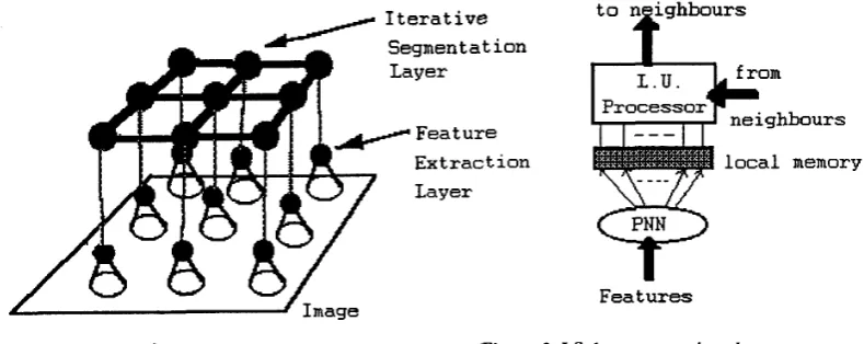
The iterative segmentation network is essentially a hybrid two-layer neural network. Figure 1 shows the basic network structure. The first layer of processing elements (P.E.s) is the feature extraction Zuyer and each P.E. in this layer has a receptive field, which encompasses a region of the image sufficiently large for feature extraction processing. The function of each P.E. can be as simple as passing the pixel intensity to the next layer, or it may involve the extraction of more complex features such as texture or moments. Regardless of the features being used, tliere are always as many feature extraction processing elements as there are pixels. The presence of the receptive fields constrains the feature extraction process to be an inherently local operation and hence there is no requirement for communication between the P.E.s in this layer.
Iterative
Segmentation Layer
M Feature
Extraction
Layer
Features
lbours
memory
1 f Image
Figure 1. Network Structure Figure 2. I.S. layer processing element
The actual structure of the processing elements in the feature extraction layer is somewhat arbitrary. Many of the common measures used in image segmentation tend be formed from linear (or at worst simple polynomial) functions of the intensity values of pixels in the receptive field and hence it has been found that perceptron-type neurons (or small networks of perceptrons) are generally sufficient in constructing P.E.s for this layer.
The second layer of the network, the iterative segrnentation layer, is considerably more complex in both its P.E. structure and its interconnection structure. It can be seen from Figure 1 that P.E.s in this layer accept feature vectors from their associated feature extraction P.E.s in the first layer as their primary input source. The primary output from each P.E. is a classification (i.e., the type of tissue) of tlie pixel to which the P.E. corresponds in the image. In addition to this, each P.E. is fully connected to its four nearest neighbours. These connections consist of
K+1
outputs to each neighbour (where K is the number of known region types in the image), and a further K+l inputs from each neighbouring P.E.. The function of these interconnects will be explained in section 3.2.Figure 2 shows the intemal structure of the processing elements which constitute the iterative segmentation layer. There are three major substructures within each P.E. - a probabilistic neural network, a block of local memory and the local update processing unit. The size of each P.E., that is, the number of intemal memory cells, interconnections, etc., will clearly be dependent upon the number of tissue classes known to be present in the image.
3.2 Network Function
The operation of the network can be broken down into two clearly distinguishable phases. The first phase involves the generation of initial states for the output of the iterative segmentation (I.S.) layer by using the feature
extraction layer and probabilistic units of the I.S. layer. In the second phase, the I.S. layer neurons interact by passing likelihood information to their neighbours in an iterative process in order to generate a globally stable segmentation result. Each of these phases will be described in more detail below.
m
m
Consider an image consisting of an MxN array of pixels, where each pixel has
an
associated intensity value, I(x,y) (in the case of MRI images this will typically be some function of the spin-spin and spin-echo relaxation times). Upon initiating the segmentation process, the feature extraction layer will generate, via processing of receptive fields centred on each pixel, an MxN array of feature vectors, F(x,y). The actual dimensionality of these vectorswill obviously be a function of the feature extraction process that is used. The feature vectors are then passed to the iterative segmentation layer, where they become inputs to the probabilistic neural network (P") units which have been previously trained to process the particular input features being used. As outlined in section 2, the PNNs used in this particular network differ from those typically used in most classification tasks, in that they do not classify the input vector but instead produce a vector of likelihoods representing the likelihood that each of the known segmentation classes could have generated the input feature vector, F(x,y). These initial likelihood estimates, Lo(x,y), are then placed into each P.E.'s local memory and an initial classification is generated by the local update processor by taking the class with the highest liielihood.
Phase 2: Iterative Segmentation
Once initial estimates of the likelihoods for each pixel have been computed, the feature extraction layer is disabled and the iterative segmentation layer operates independently by adjusting the likelihoods associated with each P.E. based upon information it receives from neighbouring P.E.s in an iterative manner. This process continues until a suitable stopping criterion bas been reached. The final segmented image is then generated by choosing the class with the maximum likelihood value at each P.E. as the most likely true class of the associated pixel.
The iterative segmentation process can be broken down into five basic steps, which are described below.
Step 1: For each P.E., calculate a confidence factor, c(x,y), to represent the confidence that the P.E. has in its current classification. There are obviously a great number of measures that could be used to define such a confidence factor. The particular measure described here is formed by taking the maximum likelihood value (the current classification), L-(x,y), and the second highest likelihood value, L,,(x,y) and forming
-
This produces a measure that ranges between 0 (when L,, =
LM)
and 1 (when L,, >>LM)
which can then be used to modulate the influence of information from neighbouring P.E.s and to determine how much relative influence the P.E. has upon its neighbours.Step 2: Each P.E. broadcasts to its four nearest neighbours its likelihood vector and its confidence factor. Hence, as mentioned in the previous section, between a P.E. and each of its neighbours there are K+l output connections for broadcasting information (likelihood vector of dimension K plus one for the confidence factor) and K+l input connections for receiving information.
Step 3: Each of the P.E.s updates its likelihood estimates based upon its own confidence about its current
state,
and the confidence that the neighbouring P.E.s have about their current states. Essentially, if a P.E. hasa
high confidence factor then it should not change its likelihood estimates greatly, but when the confidence is low, it should rely heavily on the information it receives from neighbouring P.E.s to update its estimates. The update is c'uried out by the local update unit, where each component of the likelihood vector is updated independently. That is, the likelihood estimate for class k is only modified by the class k estimates of its neighbours, without any explicit dependence upon the likelihoods of other classes.In the present implementation of the network, the dynamic being used is
-
where D is the neighbourhood about (x,y)
Thus, the likelihoods are modified by retaining a proportion of the current likeliioods equal to the confidence factor of the P.E. and then adding a weighted sum of the likelihood values of the neighbouring P.E.s. There are two components to this weighting: The first component, (1
-
c(x,y)), is simply the amount of uncertainty that theP.E. has about its own values and tlie second component, the c(m,n)s, are the certainty factors of the neighbouring
P.E.s. Hence, a P.E. with a low certainty factor will be most heavily influenced by the surrounding P.E.s which have the greatest certainty factors. Once the likelihood values for all of the classes have been updated, the new values are placed into the local memory of the P.E.,
Step 4: After all likelihood values have been recalculated, the final step is to decide whether the network has converged sufficiently, or whether another iteration is required. There are many possible stopping conditions that may be suitable, and the one used in this particular case is to stop when less than a predetermined percentage of
P.E.s change their classification decision. If tliis condition is not satisfied then another iteration is performed from step 1.
Step 5: At tliis point the network has converged and the final segmentation is determined by each P.E. choosing the class with tlie maximum likelihood.
4.
Simulation Results
The network has been applied to the task of segmenting several
h4RI
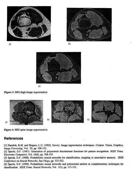
images. Figure 3a is a single echo h4RI image of a human thigh. The network was trained to distinguish three tissue types-
bone, muscle and other tissue using only the pixel intensity. The results of the initialisation phase are shown in Figure 3b and the final segmentation result after 17 iterations is shown in Figure 3c. While there is a misclassification of a region of the muscle tissue as bone in the top section of the muscle, the overall result is quite satisfactory and vastly superior to attempts to segment this image with conventional algorithms.A substantially more difficult image is shown in Figure 4a. This is a cross-section through a human vertebra suspended in a saline solution. Once again, the segmentation classes were bone, muscle and other tissue, and the pixel intensity was used as the segmentation feature. Figure 4b shows the initial segmentation and the final result after 26 iterations is shown in Figure 4c. Altliough the segmented image is still relatively crude, it is a particularly good result considering the complexity of the original image. Further improvement will most likely be made by constructing better features for the initial segmentation phase.
5.
Conclusions
An iterative segmentation network based upon tlie probabilistic neural network has been presented. It has been shown Uiat an iterative process which utilises likelihood estimates generated by the
PNN
at each pixel can lead to a segmentation result that does not rely heavily on the quality of the initial segmentation. Two examples using actualMRI
images have shown tliat this preliminary investigation could lead to a network suitable for tasks such as volumetric tissue analysis wliicli require an accurate image segmentation system.C)
Figure 3. MRI thigh image segmentation
Figure 4.
MRI
spine image segmentation.References
[I] Hmalick,
R.M.
and Shapiro, L.G. (1985). Survey: Image segmentation techniques. Comput.Vision,
Gruphics, h u g e Processing, Vol .29, pp. 100-132.[2] Speclit, D.F. (1967). Generation of polynomial discriminant functions for pattem recognition. ZEEE Trans. Electronic Computers, Vol. 16(8), pp. 308-3 19.
[3] Specht, D.F. (1988). Probabilistic neural networks for classification, mapping or associative memory. IEEE Conference on Neurul Networks, San Diego, pp. 525-532.