Vol. 10, No. 2, 2018 Article ID IJIM-00818, 16 pages Research Article
A Note On Dual Models Of Interval DEA and Its Extension To
Interval Data
H. Azizi ∗, A. Amirteimoori †‡, S. Kordrostami §
Received Date: 2016-01-14 Revised Date: 2016-05-05 Accepted Date: 2017-06-20
————————————————————————————————–
Abstract
In this article, we investigate the measurement of performance in DMUs in which input and/or output values are given as imprecise data. By imprecise data, we mean that in some cases, we only know that the actual values are inside certain intervals, and in other cases, data are specified only as ordinal preference information. In this article, we present two distinct perspectives for determining the upper and lower bounds of the efficiency the DMU under evaluation can have with imprecise data: (1) The optimistic perspective, which uses DEA-efficient production frontier, and seeks the best score among various values of the efficiency score; the measured efficiency in this perspective is called the best relative efficiency or the optimistic efficiency. (2) The pessimistic perspective, which uses inefficiency frontier, also called input frontier, and seeks the lowest score among various values of the efficiency score; the measured efficiency in this perspective is called the worst relative efficiency or the pessimistic efficiency. For this reason and contrary to some DEA-related studies, we do not restrict our attention only to precise data. We will investigate a more general case of dealing with imprecise data, providing a method for obtaining the upper and lower bounds of efficiency. Two numerical examples will be presented to illustrate the application of the proposed DEA approach.
Keywords : Data envelopment analysis; Imprecise data; Optimistic efficiency interval; Pessimistic efficiency interval; Overall efficiency interval; Ranking.
—————————————————————————————————–
1
Introduction
D
asively used to evaluate and estimate the ef-ta envelopment analysis (DEA) is exten-ficiency of decision-making units (DMUs). DEA was first proposed by Charnes et al. [1]. It has∗Department of Mathematics, Lahijan Branch, Islamic
Azad University, Lahijan, Iran.
†Corresponding author. [email protected],
Tel:+98(911)1346054.
‡Department of Mathematics, Rasht Branch, Islamic
Azad University, Rasht, Iran.
§Department of Mathematics, Lahijan Branch, Islamic
Azad University, Lahijan, Iran.
been widely used for evaluating the relative ef-ficiency of many decision-making entities in the public and private sectors. In recent years, nu-merous studies have been conducted on the ap-plication of DEA in educational and industrial centers [2,3,4].
DEA calculates an efficiency score for each DMU relative to a set of DMUs. DEA efficiency score (in input-oriented mode) defines the maxi-mum possible proportional reduction in input us-age with constant output level for each DMU. This increases the efficiency of a DMU up to the most efficient DMUs in the DMUs set. In other
words, DEA chooses a set of the most favorable weights for each DMU under evaluation. Accord-ingly, the method proposed by Charnes et al. [1] measures the efficiency of DMUs from the opti-mistic viewpoint. The measured efficiency of this method is called thebest relative efficiencyor the optimistic efficiencywhere its value is less than or equal to one. If the optimistic efficiency of a DMU is equal to one, it is DEA-efficient or optimistic efficient; otherwise, it is DEAnon-efficient or op-timistic non-efficient. It is believed that the per-formance of optimistic efficient DMUs is higher than that of optimistic non-efficient DMUs.
On the other hand, the approach proposed by Parkan and Wang [5] measures the efficiency of DMUs from the pessimistic viewpoint [6, 7]. In this approach, a set of the most unfavorable weights is selected for each DMU under evalua-tion. The measured efficiency of the pessimistic perspective is called the worst relative efficiency or the pessimistic efficiency where its value is greater than or equal to one. If the pessimistic efficiency of a DMU is equal to one, that DMU is called pessimistic inefficient or DEA-inefficient; otherwise it is called pessimistic non-inefficient or DEAnon-inefficient. It is commonly believed that the performance of the pessimistic ineffi-cient DMUs is worse than the pessimistic non-inefficient DMUs.
Optimistic and pessimistic efficiencies measure two extremes of the performance of each DMU. Any method that considers only one of the per-spectives is bias. To determine the overall perfor-mance of DMUs, both optimistic and pessimistic viewpoints should be considered simultaneously.
Entani et al. [8] proposed a paired DEA model with interval efficiencies measured from both op-timistic and pessimistic perspectives. The paired DEA model was initially developed for crisp data and later was extended to interval and fuzzy data. Theoretically, their models were able to render both interval and fuzzy data. However, there were some problems with the models. The models only use one input and one output data to deter-mine the lower bound of the efficiency interval for each DMU regardless of the number of inputs and outputs in the model. Consequently, their model leads to data loss concerning input and output data of the DMU under evaluation. In addition,
the paired DEA model uses variable production frontiers to measure the efficiency intervals of dif-ferent DMUs with interval data. Wang and Yang [9] proposed a pair of bounded DEA model for crisp data. The pair of bounded DEA model uses all possible inputs and outputs. It mea-sures the best and the worst relative efficiencies of each DMU using a virtual DMU called anti-ideal DMU. The anti-ideal DMU employs the maxi-mum input value to produce the minimaxi-mum out-put. The efficiency of an anti-ideal DMU is zero when all output values are zero. As a result, their pair of bounded DEA model fails when deter-mining the interval efficiency for each DMU. Re-cently, Azizi and Wang [10] developed improved bounded DEA models which are able to measure the efficiencies of DMUs in all situations. Wang et al. [11] proposed a pair of interval DEA model for precise data. The interval DEA models use the pessimistic efficiency of a virtual DMU called ideal DMU- which employs the minimum input to produce the maximum output- for determin-ing the efficiency interval for each DMU. Accord-ingly, the optimistic and pessimistic efficiencies of each DMU are measured. Accordingly, Azizi and Jahed [12] noted that the interval DEA mod-els of Wang et al. [11] are unable to determine the lower bound of the efficiency interval for each DMU when the input value is zero. To resolve this problem, Azizi and Jahed [12] developed an im-proved interval DEA model to measure the over-all performances of DMUs in over-all conditions. Azizi and Fathi Ajirlu [13] used the optimistic efficiency of the ideal DMU and the pessimistic efficiency of the anti-ideal DMU to determine the lower bound of the efficiency interval for crisp data. Their DEA models were unable to determine the lower bound of the efficiency interval when there were zeros in each input and output. Foroughi and Aouni [14] proposed a mixed integer linear pro-gramming model to determine the lower bound of the efficiency interval for each DMU. The pro-posed model is unable to identify all pessimistic inefficient DMUs.
efficien-cies, they defined two virtual DMUs called ideal DMU and anti-ideal DMU to develop two DEA models. They combined these two distinct effi-ciencies and obtained a relative closeness index as a basis for ranking DMUs. Their proposed DEA models have two major disadvantages: (1) In most cases, their DEA models use constant weights for all DMUs, and (2) when there are ze-ros in each input and output, their DEA models are infeasible. Wang et al. [16] proposed a ge-ometric average efficiency measure to assess the overall performance of each DMU. The geometric average efficiency combines both optimistic and pessimistic efficiencies of each DMU. Therefore, it is more comprehensive than either of the mea-sures. Recently, Wang and Lan [17] and Chin et al. [18] extended this approach. Wang and Chin [19] proposed a new overall performance measure for ranking DMUs. The proposed DEA approach considers both optimistic and pessimistic efficien-cies of the DMUs simultaneously. The overall performance measure not only considers the mag-nitude of the two different efficiencies, but also considers their directions. Therefore, it is as-sumed to be more comprehensive than the ge-ometric average efficiency measure proposed by Wang et al. [16]. Amirteimoori [20] introduced an efficiency measure using the ideal and anti-ideal indicators formed on the basis of the efficient and inefficient frontiers of the DEA. These indi-cators maximize of the weightedL1distance from a particular DMU relative to the inefficient and efficient frontiers of the DEA. Amirteimoori et al. [21] also improved the cost efficiency interval of a DMU by adjusting the observed inputs and out-puts. Based on returns to scale terms, Wang and Lan [22] examined the most productive scale size of a DMU from both optimistic and pessimistic perspectives.
According to literature, much effort is needed to measure the overall performances of DMUs, because it should be measured in a more general case in the presence of imprecise data. It is note-worthy that the papers concerning the simultane-ous application of both optimistic and pessimistic viewpoints were reviewed. Entani et al. [8] ex-amined the DEA structure in the presence of in-terval data from both optimistic and pessimistic perspectives. The drawbacks of DEA models are
described in Section 3. The main objective of the present paper is to measure the overall per-formances of DMUs using DEA and simultane-ous application of crisp, ordinal and interval data. The upper bound of the overall efficiency interval is obtained from the optimistic viewpoint based on the best position of each DMU using a set of the most favorable weights. The lower bound is obtained from the pessimistic viewpoint based on the most unfavorable position of each DMU using a set of the most unfavorable weights. The overall efficiency interval shows all possible evaluations through different perspectives. Accordingly, the decision maker is provided with the efficiency in-terval of all possible values of efficiencies reflect-ing the different views. Two numerical examples illustrate the application of the proposed method. Since the ultimate efficiency score for each DMU is characterized by an interval, a simple but prac-tical ranking approach is needed to rank and compare DMUs efficiencies. Previously, several approaches have been developed to rank inter-val numbers. But all of them have some disad-vantages. In particular, when the interval num-bers have equal centers but different widths, all of them are incapable of distinguishing between these numbers. We use the minimax regret ap-proach, developed by Wang et al. [23], for com-paring and ranking the efficiency intervals of the DMUs.
This paper is organized as follows. Section 2 in-troduces the basic DEA models used for deter-mining the best and the worst relative efficiencies of DMUs. Section 3 analyzes the DEA models proposed by Entani et al. [8], then the adjusted pessimistic efficiency interval is reviewed. Section
2
Interval DEA models for
mea-surement of the best and the
worst relative efficiencies
2.1 Interval DEA models for measure-ment of the best relative efficien-cies of DMUs
In DEA analysis, it is usually assumed that there are nproduction units that consume m different inputs and produce s different outputs. Specifi-cally, the jth production unit consumes xij units
of input i (i = 1, . . . , m) and produces yrj units
of output r (r = 1, . . . , s). In interval DEA, it is assumed that some exact values of input xij and output yrj are not known. It is only
known that they are in the range of the upper and lower bounds specified by intervals [xLij, xUij] and [yLrj, yUrj], and each DMU has a positive lower bound input and a positive lower bound output. To deal with such an uncertain situation, Wang et al. [23] presented the following pair of linear programming (LP) models that measure the best relative efficiencies of DMUs:
max θUo =
s
∑
r=1 uryroU
s.t.
s
∑
r=1
uryrjU − m
∑
i=1
vixLij ≤0, j= 1, . . . , n,
m
∑
i=1
vixLio = 1,
ur, vi ≥ε, r= 1, . . . , s;i= 1, . . . , m.
(2.1)
max θLo =
s
∑
r=1 uryLro
s.t.
s
∑
r=1
uryrjU − m
∑
i=1
vixLij ≤0, j= 1, . . . , n,
m
∑
i=1
vixUio = 1,
ur, vi ≥ε, r= 1, . . . , s;i= 1, . . . , m.
(2.2) where DMUo is the DMU under evaluation, vi
(i = 1, . . . , m) and ur (r = 1, . . . , s) are
deci-sion variables, and ε is the non-Archimedean in-finitesimal [24]. θoU is the best relative efficiency under the most favorable conditions and θLo is
the best relative efficiency under the most un-favorable conditions for DMUo. They form the
optimistic efficiency interval [θLo, θUo]. If there is a set of positive weights u∗r (r = 1, . . . , s) and vi∗ (i = 1, . . . , m) that make θoU∗ = 1, then DMUo is called DEA-efficient or optimistic
effi-cient; otherwise, it is called DEA-non-efficient or optimistic non-efficient. All DEA-efficient DMUs collectively form an efficiency frontier.
2.2 Interval DEA models for measure-ment of the worst relative efficien-cies of DMUs
The input-orientedframework, which is based on the set of input requirement and its inefficiency frontier, tries to increase input values as much as possible, while keeping the output at most at its current level. This emphasizes the fact that output is kept constant and input values are in-creased proportionally, until the inefficient pro-duction frontier is obtained. DEA estimator for inefficient production possibility set is called the pessimistic efficiency or the worst relative effi-ciency. For a particular DMU, such as DMUo,
relative efficiencies can be calculated form the fol-lowing pessimistic DEA models [25]:
minϕLo =
s
∑
r=1 uryroL
s.t.
s
∑
r=1
uryLrj− m
∑
i=1
vixUij ≥0, j= 1, . . . , n,
m
∑
i=1
vixUio = 1,
ur, vi≥ε, r= 1, . . . , s;i= 1, . . . , m.
(2.3)
minϕUo =
s
∑
r=1 uryroU
s.t.
s
∑
r=1
uryLrj− m
∑
i=1
vixUij ≥0, j= 1, . . . , n,
m
∑
i=1
vixLio = 1,
ur, vi≥ε, r= 1, . . . , s;i= 1, . . . , m.
condi-Table 1: Data for five DMUs with one input and one output.
DMU Input Output
A [1, 3] [2, 3]
B [4, 5] [6, 7]
C [9, 11] [7, 9]
D [6, 8] [1, 3]
E [5, 7] [4, 5]
tions andϕUo is the worst relative efficiency under the most favorable conditions for DMUo. They
give the pessimistic efficiency interval [ϕL
o, ϕUo] for
DMUo. When there is a set of positive weightsu∗r
(r = 1, . . . , s) and vi∗ (i= 1, . . . , m) that satisfy ϕLo∗ = 1, we say that DMUo is DEA-inefficient
or pessimistic inefficient; otherwise, we say that DMUo is DEA-inefficient or pessimistic
non-inefficient. All DEA-inefficient DMUs collectively form an inefficiency frontier.
In order to illustrate the difference between
op-A B
C
D E
Input Output
Efficiency frontier
Inefficiency frontier
Figure 1: Efficiency and inefficiency frontiers for the five DMUs under variable return to scale.
timistic efficient, optimistic non-efficient, pes-simistic inefficient, and pespes-simistic non-inefficient DMUs (i.e., the difference between the efficiency frontier and the inefficiency frontier), we use an example of a dataset with one input and one out-put, as shown in Table 1. The efficiency and in-efficiency frontiers for this example are shown in Figure 1. As it is clear from the figure, three DMUs are on the efficient frontier, which we call DEA-efficient or optimistic efficient DMUs, and the rest of the DMUs are called DEA-non-efficient or optimistic non-efficient in relation to the effi-cient frontier. Also, there are two DMUs on the inefficient frontier, which we call DEA-inefficient
or pessimistic inefficient, while we call the rest of the DMUs DEA-non-inefficient or pessimistic non-inefficient in relation to the inefficient fron-tier. Here, there is also some overlap, or common units, between optimistic efficient and pessimistic inefficient units.
3
The overall efficiency
interval-Integration of the optimistic
and pessimistic efficiencies
3.1 A review of Entani et al.’s [8] DEA models
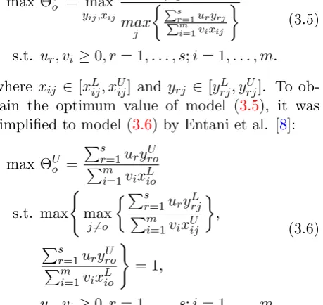
To develop an overall efficiency interval for each DMU, Entani et al. [8] proposed the following mathematical programming model to determine the upper bound of the overall efficiency interval of DMUo:
max ΘUo = max
yij,xij
∑s r=1uryro ∑m
i=1vixio
max
j
{∑
s r=1uryrj ∑m
i=1vixij }
s.t. ur, vi≥0, r= 1, . . . , s;i= 1, . . . , m.
(3.5)
where xij ∈ [xLij, xUij] and yrj ∈ [yrjL, yrjU]. To
ob-tain the optimum value of model (3.5), it was simplified to model (3.6) by Entani et al. [8]:
max ΘUo =
∑s
r=1uryroU
∑m i=1vixLio
s.t. max
{
max
j̸=o
{∑s
r=1uryrjL
∑m i=1vixUij
}
,
∑s
r=1uryroU
∑m i=1vixLio
}
= 1,
ur, vi≥0, r= 1, . . . , s;i= 1, . . . , m.
(3.6)
problem:
max ΘUo =
s
∑
r=1 uryroU
s.t.
s
∑
r=1
uryrjL − m
∑
i=1
vixUij ≤0, j= 1, . . . , n;j̸=o,
s
∑
r=1
uryroU − m
∑
i=1
vixLio≤0,
m
∑
i=1
vixLio = 1,
ur, vi ≥ε, r= 1, . . . , s;i= 1, . . . , m.
(3.7) In models (3.6) and (3.7), the lower bounds of input intervals xLio and the upper bounds of out-put intervals yUro are used for DMUo, and
up-per bounds of input intervals xUij and the lower bounds of output intervalsyrjL are used for other DMUs. Model (3.7) is equivalent to the up-per bound DEA model of Despotis and Smirlis [26], and reports many DMUs that are not DEA-efficient as DEA-DEA-efficient. One of the drawbacks of model (3.7) is that it uses different constraint sets for evaluating the efficiencies of different DMUs. The main drawback of using different sets of constraints for efficiencies measurement of DMUs is the lack of possibility of compari-son between efficiencies, since different produc-tion frontiers have been used in the process of efficiency measurement. We use LP model (2.1) for obtaining the upper bound of the overall effi-ciency interval for each DMU. This model is dif-ferent from the existing DEA models for interval data in that the LP model (2.1) uses a fixed and unified production frontier for measuring the effi-ciency of each DMU. To obtain the lower bound of the overall efficiency interval for DMUo, Entani
et al. [8] proposed the following mathematical programming model for DMUo:
minφLo = min
yij,xij ∑s
r=1uryro ∑m
i=1vixio
max
j { ∑s
r=1uryrj ∑m
i=1vixij}
s.t. ur, vi≥0, r= 1, . . . , s;i= 1, . . . , m.
(3.8)
To obtain the optimum value of model (3.8), it was simplified to model (3.9) by Entani et al. [8]:
min φLo =
∑s
r=1uryLro
∑m i=1vixUio
s.t. max
{
max
j̸=o
{∑s
r=1uryrjU
∑m i=1vixLij
}
,
∑s
r=1uryLro
∑m i=1vixUio
}
= 1,
ur, vi ≥0, r= 1, . . . , s;i= 1, . . . , m.
(3.9)
The upper bounds of the input intervals, xUio and the lower bounds of the output intervals, yroL in model (3.9) are used for DMUo. The
lower bounds of the input intervals, xLij and the upper bounds of the output intervals, yrjU are used for other DMUs. Model (3.9) cannot be transformed into an equivalent LP model. To achieve the optimal value of model (3.9), assum-ing ∑sr=1uryUrj/
∑m
i=1vixLij = 1 for each
DEA-efficient unit, Entani et al. [8] divided. Model (3.9) into e1 sub-optimization problems j = J1, . . . , Je1, in which e1 is the number of
DEA-efficient units, and J1, . . . , Je1 are DEA-efficient
units:
minφLoj =
∑s
r=1uryLro
∑m i=1vixUio
s.t.
∑s
r=1uryUrj
∑m i=1vixLij
= 1,
ur, vi≥0, r= 1, . . . , s;i= 1, . . . , m.
(3.10)
The sub-optimization problem (3.10) can be con-verted toe1 LP models as follows:
minφLoj =
s
∑
r=1 uryroL
s.t.
s
∑
r=1
uryUrj− m
∑
i=1
vixLij = 0,
m
∑
i=1
vixUio = 1
ur, vi≥0, r= 1, . . . , s;i= 1, . . . , m.
(3.11)
Entani et al [8] claim that the minimum value out of the optimal values of (3.11) is the optimal value of model (3.9). Assuming thatφLoJ∗
1, . . . , φ
the optimal values of the objectives functions in LPs of the sub-optimization problem (3.11), we can write the lower bound of the overall efficiency interval of DMUo mathematically as follows:
φLo∗ = min
j=J1,...,Je1
{φLoj∗} (3.12)
Accordingly, [φLo∗,ΘUo∗] is the overall efficiency in-terval of DMUo, where ΘUo∗ is the optimal value
of model (3.7).
In the sub-optimization problem (3.11), each LP model has only two linear constraints. There-fore, regardless of the number of inputs and out-puts in the problem under consideration, only two decision variables can be non-zero, one for the in-put weight and the other for the outin-put weight. As such, Entani et al.’s [8] DEA models mea-sure the pessimistic efficiency of each DMU by taking into account only one input and one out-put. Compared with the sub-optimization prob-lem (3.11), model (2.3) includes (n+ 1) linear constraints and, consequently, can make the most use of input and output information. Addition-ally, model (2.3) is able to accurately identify the pessimistic inefficient units and the inefficiency frontier. To clarify this point, consider the fol-lowing numerical example.
Example 3.1 Consider the example discussed by Cooper et al. [27]. We have five DMUs that use two inputs, one crisp and the other interval, and produce two outputs, one crisp and the other ordinal. The data set is shown in Table 2.
For conversion of ordinal preference information into interval data, we used the approach proposed by Wang et al. [23]. For this example, the prefer-ence intensity parameter and the ratio parameter about the strong ordinal preference information were determined (or estimated) as χ2 = 1.2 and σ2 = 0.2, respectively [28, 29]. Using the tech-nique described in Wang et al. [23], we can ob-tain an interval estimate for the second output of each DMU, which is shown in the last column of Table2.
First we obtain the optimistic and pessimistic ef-ficiencies of the five DMUs using interval DEA models (2.1)-(2.4). These are shown in Table 3. From Table 3, it is clear that only one DMU,
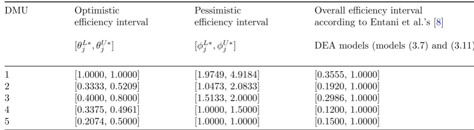
i.e. DMU1, is DEA-efficient according to the op-timistic DEA model (2.1). This DEA-efficient unit determines the efficiency frontier. It is usu-ally believed that this DEA-efficient unit should have a better performance than the other four units that are identified as DEA-non-efficient. From the pessimistic efficiency perspective, two DMUs, i.e. DMU4 and DMU5, are identified as DEA-inefficient. Collectively, they define an inefficiency frontier. It is believed that these two DEA-non-efficient units have a poorer perfor-mance than the three units that are identified as DEA-non-inefficient. The evaluations above have been performed from different perspectives and, as such, may have different results. Any conclu-sion based on only one of these two perspectives will undoubtedly be unrealistic and unconvinc-ing. In order to provide an overall assessment of the performance of each DMU, Entani et al. [8] considered both optimistic and pessimistic per-spectives simultaneously. The results of Entani et al.’s [8] interval DEA models are shown in the last column of Table 3. As it can be seen from Table 3, due to the use of different production frontiers for measuring the efficiencies of different DMUs, model (3.7), which is used by Entani et al. [8] for obtaining the upper bound of the over-all efficiency interval, evaluates over-all five DMUs as DEA-efficient. Also, the sub-optimization prob-lem (3.11), which is used by Entani et al. [8] for obtaining the lower bound of the overall effi-ciency interval, identifies only DMU4, which has the smallest lower-bound efficiency among the five DMUs, as a DEA-inefficient unit. But it cannot identify DMU5 which is DEA-inefficient. Consequently, the efficiency and inefficiency fron-tiers cannot be determined using Entani et al.’s [8] interval DEA models.
Table 2: Imprecise data and ordinal data converted for five DMUs.
DMU Inputs Outputs Converted ordinal data
x1j (exact) x2j (interval) y1j (exact) y2j (ordinal⋆)
1 100 [0.6, 0.7] 200 4 [0.3456, 0.8333] 2 150 [0.8, 0.9] 1000 2 [0.2400, 0.5787]
3 150 [1, 1] 1200 5 [0.4147, 1.0000]
4 200 [0.7, 0.8] 900 1 [0.2000, 0.4823]
5 200 [1, 1] 600 3 [0.2880, 0.6944]
⋆ Ranking, such that 5≡highest rank,. . ., 1≡lowest rank (y
23≻y21≻ · · · ≻y24)
Table 3: Imprecise data and ordinal data converted for five DMUs.
DMU Optimistic Pessimistic Overall efficiency interval efficiency interval efficiency interval according to Entani et al.’s [8] [θjL∗, θUj∗] [ϕLj∗, ϕUj∗] DEA models (models (3.7) and (3.11)
1 [1.0000, 1.0000] [1.9749, 4.9184] [0.3555, 1.0000] 2 [0.3333, 0.5209] [1.0473, 2.0833] [0.1920, 1.0000] 3 [0.4000, 0.8000] [1.5133, 2.0000] [0.2986, 1.0000] 4 [0.3375, 0.4961] [1.0000, 1.5000] [0.1200, 1.0000] 5 [0.2074, 0.5000] [1.0000, 1.0000] [0.1500, 1.0000]
LP models must be solved:
(LP1): φL31∗= min 1200u1+ 0.4147u2
s.t.
150v1+v2 = 1,
2000u1+ 0.8333u2−100v1−0.6v2 = 0, u1, u2, v1, v2≥0.
(LP2): φL32∗= min 1200u1+ 0.4147u2
s.t.
150v1+v2 = 1,
1000u1+ 0.5787u2−150v1−0.8v2 = 0, u1, u2, v1, v2≥0.
(LP3): φL∗33 = min 1200u1+ 0.4147u2
s.t.
150v1+v2= 1,
1200u1+u2−150v1−v2 = 0, u1, u2, v1, v2≥0.
(LP4): φL34∗= min 1200u1+ 0.4147u2
s.t.
150v1+v2 = 1,
900u1+ 0.4823u2−200v1−0.7v2 = 0, u1, u2, v1, v2≥0.
(LP5): φL35∗= min 1200u1+ 0.4147u2
s.t.
150v1+v2 = 1,
600u1+ 0.6944u2−200v1−v2= 0, u1, u2, v1, v2 ≥0.
The solutions of these five LP models are as fol-lows:
φL∗31 = 0.2986, u∗1 = 0, u∗2 = 0.7200, v1∗ = 0 and v∗2 = 1,
φL32∗ = 0.5733, u∗1 = 0, u∗2 = 1.3824, v1∗ = 0 and v∗2 = 1,
φL33∗ = 0.4147, u∗1 = 0, u2∗ = 1, v1∗ = 0 and v2∗ = 1,
φL∗34 = 0.6019, u∗1 = 0, u∗2 = 1.4514, v1∗ = 0 and v∗2 = 1,
φL35∗ = 0.5972, u∗1 = 0, u∗2 = 1.4401, v1∗ = 0 and v∗2 = 1.
Finally, the lower bound of the overall efficiency interval of DMU3 is obtained as follows:
φL3∗ = min{0.2986,0.5733,0.4147,
0.6019,0.5972}= 0.2986
u∗1 = 0, u∗2 = 1.4514, v1∗ = 0, v2∗ = 1. We sub-stituted this set of weights in the constraints of model (9) and obtained the following efficiencies for the DMUs:
φL1∗ = 2.0158, φL2∗ = 1.0499, φL3∗ = 1.4514, φL4∗ = 0.3629, φL5∗ = 1.0079.
Except for the efficiency of DMU4, all other efficiency values are greater than one. Such results evidently violate the con-dition max
{
max
j̸=o{
∑s
r=1uryLrj/
∑m
i=1vixUij},
∑s
r=1uryroU/
∑m i=1vixLio
}
= 1. Therefore, the
approach proposed by Entani et al. [8] for ob-taining the lower bound of the overall efficiency interval is illogical and unacceptable.
In the next section, we will develop novel DEA models for determination of the lower bound of the overall efficiency interval in order to overcome these drawbacks.
The pessimistic efficiency score is the opposite of the optimistic efficiency score. It is a score that each DMU obtains in its most unfavorable situa-tion (or the most favorable situasitua-tion) using a set of the most unfavorable weights. Theoretically, the best and the worst relative efficiencies should be calculated in a common range and should form an interval for each DMU. For example, they can be measured in the interval [β,1], whereβ >0 is a parameter. In the next section, we will find a suitable value forβ.
3.2 Adjusting the worst relative effi-ciencies
Theoretically, the best and the worst relative ef-ficiencies should form an interval. For this pur-pose, the worst relative efficiencies determined by models (2.3) and (2.4) should be adjusted [30,31]. Suppose thatβ (0< β≤1) is the adjustment co-efficient, then the adjusted worst relative efficien-cies can be written asβϕ∗j =β[ϕL∗
j , ϕUj∗] = ˆϕ∗j =
[ ˆϕLj∗,ϕˆjU∗] (j = 1, . . . , n) satisfying ˆϕ∗j = βϕ∗j = β[ϕjL∗, ϕUj∗] ≤ θj∗ = [θjL∗, θjU∗] (j = 1, . . . , n) or β ≤ min
j=1,...,n{θ L∗
j /ϕUj∗}. Assuming ϕUmax∗ =
max
j=1,...,n{ϕ U∗
j } and θLmin∗ = j=1min,...,n{θjL∗}, then
min
j=1,...,n{θ L∗
j /ϕUj∗} ≥ j=1min,...,n{θjL∗}/ maxj=1,...,n{ϕUj∗}.
Substituting β = θLmin∗ /ϕUmax∗ , it is ensured that
β ≤ min
j=1,...,n{θ L∗
j /ϕUj∗}. Since β is not zero, the
worst performance of DMUs in the interval [β,1] can be measured by the following models:
min ΨLo =
∑s
r=1uryLro
∑m i=1vixUio
s.t.
∑s
r=1uryLrj
∑m i=1vixUij
≥β, j= 1, . . . , n,
ur, vi ≥ε, r= 1, . . . , s;i= 1, . . . , m.
(3.13)
min ΨUo =
∑s
r=1uryroU
∑m i=1vixLio
s.t.
∑s
r=1uryLrj
∑m i=1vixUij
≥β, j= 1, . . . , n,
ur, vi ≥ε, r= 1, . . . , s;i= 1, . . . , m.
(3.14)
Models (3.13) and (3.14) can be transformed into the following two LP models:
min ΨLo =
s
∑
r=1 uryroL
s.t.
s
∑
r=1
uryrjL − m
∑
i=1
vi(βxUij)≥0, j= 1, . . . , n,
m
∑
i=1
vixUio = 1
ur, vi ≥ε, r = 1, . . . , s;i= 1, . . . , m.
(3.15)
min ΨUo =
s
∑
r=1 uryUro
s.t.
s
∑
r=1
uryrjL − m
∑
i=1
vi(βxUij)≥0, j= 1, . . . , n,
m
∑
i=1
vixLio = 1
ur, vi ≥ε, r = 1, . . . , s;i= 1, . . . , m.
this reason, the optimistic and pessimistic effi-ciency intervals of DMUs are merged to obtain a new interval called theoverall efficiency interval. Both upper and lower bounds (extreme values) of the overall efficiency interval are considered from two different viewpoints. As a result, an over-all efficiency interval of [ΨLj∗,ΨUj∗] (j= 1, . . . , n) is defined for each DMUj. The upper bound of
the overall efficiency interval is obtained from the optimistic viewpoint based on the best position of each DMU using a set of the most favorable weights. The lower bound is obtained from the pessimistic viewpoint based on the most unfavor-able position of each DMU using a set of the most unfavorable weights. The overall efficiency inter-val shows all possible einter-valuations of different per-spectives. Accordingly, the decision maker is pro-vided with the overall efficiency interval of all pos-sible efficiencies reflecting different perspectives.
The following definitions are concerned for the overall efficiency interval, [ΨLo∗, θoU∗].
Definition 3.1 DMUo is called DEA-efficient or optimistic efficient, if θU∗
o = 1, otherwise it is called DEA-non-efficient.
Definition 3.2 DMUo is called DEA-inefficient or pessimistic inefficient, if ΨL∗
o = β, otherwise it is called DEA-non-inefficient.
Definition 3.3 DMUo is called DEA-unspecified if and only if it is neither DEA-efficient nor DEA-inefficient.
Regarding DEA-unspecified units, we could say that they are always circumscribed between the efficient and inefficient frontiers (see DMUE in
Figure 1) [8].
For a comparison of our proposed overall ef-ficiency interval with the overall efef-ficiency inter-val obtained from Entani et al.’s [8] DEA mod-els, consider the numerical example presented in Section 3.1. First we determine the value of β using Table 3 and we obtain β = θminL∗ /ϕUmax∗ = 0.2074/4.9184 = 0.0422.
Then we run interval DEA models (3.15) and (3.16) for each DMU to obtain the adjusted pes-simistic efficiency interval for the five DMUs. By integrating the optimistic efficiency interval and the adjusted pessimistic efficiency interval
for the five DMUs, we obtain the overall perfor-mance score, i.e. the overall efficiency interval, of each DMU. Noting the obtained overall effi-ciency intervals in Table 4, it can be clearly seen that the proposed DEA approach identifies both pessimistic inefficient DMUs accurately (DMU4 and DMU5 are identified as pessimistic inefficient DMUs). These evaluation results are completely compatible with the results of the pessimistic DEA model (2.3). In this example, DMU2 and DMU3 are identified as DEA-unspecified units. Furthermore, for comparison and ranking of the overall efficiency intervals of the five DMUs, we used the minimax regret approach for calculating the maximum loss of efficiency for each DMU. The last column of Table 4shows the ranking of the five DMUs according to the overall efficiency interval, from which it can be seen that DMU1 has the best overall performance.
It should be noted that Entani et al. [8] have developed an approach for finding overall effi-ciency intervals for crisp data, interval data, and fuzzy data. However, they have not described the method of computation of the overall efficiency interval for ordinal data. Besides, they have not considered the overall efficiency interval for a mix-ture of crisp data, interval data, and ordinal data.
4
An empirical example
In this section, the DEA approach with both ef-ficient and inefef-ficient frontiers addressed in this paper is used to evaluate the performances of the commercial bank branches. In this example, the value of the non-Archimedean infinitesimal is as-sumed to beε= 10−10.
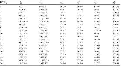
Consider, the performance measurement of 20 branches of a set of commercial bank (DMUs) in Iran. Each branch is examined in terms of three inputs including payable interest, person-nel, and non-performing loans and five outputs including the total sum of four main deposits, other deposits, loans granted, received interest, and fee. The data set used in this analysis was adopted from Jahanshahloo et al. [32]. Tables 5
pes-Table 4: Imprecise data and ordinal data converted for five DMUs.
DMU Adjusted pessimistic efficiency interval [ΨL∗
j ,ΨUj∗] Overall efficiency interval [ΨjL∗, θUj∗] Rank
1 [0.0833, 0.2076] [0.0833, 1.0000] 1
2 [0.0442, 0.0879] [0.0442, 0.5209] 3
3 [0.0639, 0.0844] [0.0639, 0.8000] 2
4 [0.0422, 0.0633] [0.0422, 0.4961] 5
5 [0.0422, 0.0422] [0.0422, 0.5000] 4
Table 5: Input data for 20 bank branches.
DMUj xL1j xU1j xL2j xU2j xL3j xU3j
1 5007.37 9613.37 36.29 36.86 87243 87243
2 2926.81 5961.55 18.8 20.16 9945 12120
3 8732.7 17752.5 25.74 27.17 47575 50013
4 945.93 1966.39 20.81 22.54 19292 19753
5 8487.07 17521.66 14.16 14.8 3428 3911
6 13759.35 27359.36 19.46 19.46 13929 15657
7 587.69 1205.47 27.29 27.48 27827 29005
8 4646.39 9559.61 24.52 25.07 9070 9983
9 1554.29 3427.89 20.47 21.59 412036 413902 10 17528.31 36297.54 14.84 15.05 8638 10229
11 2444.34 4955.78 20.42 20.54 500 937
12 7303.27 14178.11 22.87 23.19 16148 21353 13 9852.15 19742.89 18.47 21.83 17163 17290 14 4540.75 9312.24 22.83 23.96 17918 17964 15 3039.58 6304.01 39.32 39.86 51582 55136 16 6585.81 13453.58 25.57 26.52 20975 23992 17 4209.18 8603.79 27.59 27.95 41960 43103 18 1015.52 2037.82 13.63 13.93 18641 19354 19 5800.38 11875.39 27.12 27.26 19500 19569 20 1445.68 2922.15 28.96 28.96 31700 32061
simistic efficiency intervals for these DMUs based on models (2.1)-(2.4), (3.15) and (3.16). The op-timistic assessment of the bank branches revealed that 11 DMUs were in the best position and ob-tained the maximum efficiency score of 100%. These 11 DMUs are classified as optimistic ef-ficient DMUs with the best performance (best productive DMUs are DEA-efficient, otherwise they are DEA-non-efficient). However, the pes-simistic assessment of the bank branches showed that 8 DMUs were in the worst position and ob-tained the smallest efficiency score. Accordingly, these 8 DMUs are classified as pessimistic inef-ficient DMUs with the worst performance (the worst productive DMUs are DEA-inefficient, oth-erwise they are DEA-non-inefficient). These 8 DMUs are candidates for bankruptcy. Invest-ment risk assessInvest-ment is considered to be an
Table 6: Output data for 20 bank branches.
DMU yL
1j yU1j y2Lj yU2j yL3j yU3j y4Lj yU4j yL5j yU5j
1 2696995 3126798 263643 382545 1675519 1853365 108634.76 125740.28 965.97 6957.33 2 340377 440355 95978 117659 377309 390203 32396.65 37836.56 304.67 749.4 3 1027546 1061260 37911 503089 1233548 1822028 96842.33 108080.01 2285.03 3174 4 1145235 1213541 229646 268460 468520 542101 32362.8 39273.37 207.98 510.93 5 390902 395241 4924 12136 129751 142873 12662.71 14165.44 63.32 92.3 6 988115 1087392 74133 111324 507502 574355 53591.3 72257.28 480.16 869.52 7 144906 165818 180530 180617 288513 323721 40507.97 45847.48 176.58 370.81 8 408163 416416 405396 486431 1044221 1071812 56260.09 73948.09 4654.71 5882.53 9 335070 410427 337971 449336 1584722 1802942 176436.81 189006.12 560.26 2506.67 10 700842 768593 14378 15192 2290745 2573512 662725.21 791463.08 58.89 86.86 11 641680 696338 114183 241081 1579961 2285079 17527.58 20773.91 1070.81 2283.08 12 453170 481943 27196 29553 245726 275717 35757.83 42790.14 375.07 559.85 13 553167 574989 21298 23043 425886 431815 45652.24 50255.75 438.43 836.82 14 309670 342598 20168 26172 124188 126930 8143.79 11948.04 936.62 1468.45 15 286149 317186 149183 270708 787959 810088 106798.63 111962.3 1203.79 4335.24 16 321435 347848 66169 80453 360880 379488 89971.47 165524.22 200.36 399.8 17 618105 835839 244250 404579 9136507 9136507 33036.79 41826.51 2781.24 4555.42 18 248125 320974 3063 6330 26687 29173 9525.6 10877.78 240.04 274.7 19 640890 679916 490508 684372 2946797 3985900 66097.16 95329.87 961.56 1914.25 20 119948 120208 14943 17495 297674 308012 21991.53 27934.19 282.73 471.22
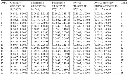
Table 7: Interval efficiencies of the 20 bank branches.
DMU Optimistic Pessimistic Pessimistic Overall Overall efficiency Rank efficiency int. efficiency int. efficiency int. efficiency int. interval according to
[θL∗
j , θUj∗] [ϕjL∗, ϕUj∗] [ΨjL∗,ΨUj∗] [ΨjL∗, θjU∗] [8] DEA models
1 [0.8561, 1.0000] [2.2649, 3.3214] [0.1049, 0.1537] [0.1049, 1.0000] [0.0024, 1.0000] 1 2 [0.3603, 0.5105] [1.8516, 2.7034] [0.0855, 0.1249] [0.0855, 0.5105] [0.0055, 1.0000] 3 3 [0.5226, 0.9802] [1.7464, 3.9815] [0.0807, 0.1840] [0.0807, 0.9802] [0.0016, 1.0000] 6 4 [0.8891, 1.0000] [1.4753, 2.4900] [0.0682, 0.1152] [0.0682, 1.0000] [0.0023, 1.0000] 9 5 [0.6331, 0.6806] [1.0000, 1.1809] [0.0462, 0.0546] [0.0462, 0.6806] [0.0009, 0.7690] 16 6 [0.8835, 1.0000] [1.6075, 3.2642] [0.0743, 0.1508] [0.0743, 1.0000] [0.0067, 1.0000] 8 7 [0.6576, 1.0000] [1.0000, 1.2160] [0.0462, 0.0562] [0.0462, 1.0000] [0.0013, 1.0000] 13 8 [0.8320, 1.0000] [1.6572, 2.8677] [0.0767, 0.1326] [0.0767, 1.0000] [0.0229, 1.0000] 7 9 [0.7396, 1.0000] [1.0000, 1.0761] [0.0462, 0.0497] [0.0462, 1.0000] [0.0003, 1.0000] 14 10 [0.8839, 1.0000] [1.0000, 1.3898] [0.0462, 0.0643] [0.0462, 1.0000] [0.0010, 1.0000] 15 11 [0.8984, 1.0000] [1.7788, 2.7646] [0.0823, 0.1279] [0.0823, 1.0000] [0.0160, 1.0000] 4 12 [0.3288, 0.3991] [1.2019, 1.6901] [0.0555, 0.0781] [0.0555, 0.3991] [0.0025, 0.4999] 12 13 [0.4438, 0.5366] [1.2225, 2.2980] [0.0565, 0.1062] [0.0565, 0.5366] [0.0026, 0.7058] 11 14 [0.2690, 0.3586] [1.0000, 1.1341] [0.0462, 0.0524] [0.0462, 0.3586] [0.0015, 0.7285] 19 15 [0.4067, 1.0000] [1.3402, 1.8771] [0.0619, 0.0867] [0.0619, 1.0000] [0.0031, 1.0000] 10 16 [0.2227, 0.5530] [1.0000, 1.5968] [0.0462, 0.0738] [0.0462, 0.5530] [0.0018, 1.0000] 17 17 [0.9871, 1.0000] [1.7289, 2.2712] [0.0807, 0.1058] [0.0807, 1.0000] [0.0084, 1.0000] 5 18 [0.2651, 0.3534] [1.0000, 1.1172] [0.0462, 0.0516] [0.0462, 0.3534] [0.0003, 0.9548] 20 19 [0.7934, 1.0000] [2.1424, 3.8900] [0.0992, 0.1801] [0.0992, 1.0000] [0.0108, 1.0000] 2 20 [0.1841, 0.4003] [1.0000, 1.0022] [0.0462, 0.0463] [0.0462, 0.4003] [0.0010, 0.9789] 18
the best DMUs. The ranking results confirm that they are not among the first 11 DMUs. Thus, the results of the present study provide more useful
It should be noted that only 80 LPs should be solved to obtain the overall efficiency interval of 20 branches using the approach proposed in this paper. To determine β, we need to be solved 20 LPs to calculate the lower bound of the opti-mistic efficiency intervals of the 20 branches (us-ing model (2.2)). On the other hand, 20 LPs should be solved to calculate the upper bound of the pessimistic efficiency intervals of the 20 branches (using model (2.4)). Of the other 40 LPs, 20 LPs are used to calculate the upper bound of the optimistic efficiency intervals of the 20 bank branches using model (2.1) (constituting the upper bound of the overall efficiency inter-vals). To calculate the lower bound of the ad-justed pessimistic efficiency intervals of the 20 bank branches (constituting the lower bound of the overall efficiency intervals), 20 LPs are solved using model (3.15). However, the DEA models proposed by Entani et al. [8] need to solve 300 LPs to obtain the overall efficiency interval of 20 branches (See Table 7). Of the 300 LPs, 20 LPs are used to calculate the upper bound of the over-all efficiency intervals of the 20 branches using model (3.7). Of this, 14 DMUs are evaluated as DEA-efficient and 20×14 LPs are used to calcu-late the lower bound of the overall efficiency inter-vals of the 20 branches using the sub-optimization problem (3.11). More importantly, the lower-bound DEA model of Entani et al. [8] identifies only one DMU, i.e. DMU9, as the pessimistic inefficient DMU with the minimum lower bound of the overall efficiency interval among the 20 DMUs. However, it is unable to detect the other seven pessimistic inefficient DMUs. The round-ing error of DMU18 is identified as a pessimistic inefficient DMU while the pessimistic efficiencies of DMU9 and DMU18are 0.000296442840994248 and 0.00030171562671364, respectively. This ex-ample confirms the applicability and discriminat-ing power of the approach proposed in this paper.
In addition to the above advantages, the other advantages of the proposed approach are as fol-lows compared with Entani et al.’s [8] approach:
• In our proposed approach, the upper bounds of the overall efficiency intervals are mea-sured according to the same constraints for dif-ferent DMUs. However, the method proposed by Entani et al. [8] measures the upper bounds of
the overall efficiency intervals under different con-straints leading to incomparable efficiencies for different DMUs.
• One of the important features of measuring the pessimistic efficiency of DMUs is identifica-tion of pessimistic inefficient DMUs which, from the pessimistic point of view, have the role of the worst units among other DMUs and delineate the inefficiency frontier. Thus, the evaluators may know which DMU is pessimistic inefficient and which is not. The lower-bound DEA model of Entani et al. [8] is an exception. Their model identifies only one DMU with the minimum lower bound of the efficiency interval. Accordingly, it is unable to correctly identify all pessimistic in-efficient DMUs. Basically, the lower-bound DEA model of Entani et al. [8] is unable to determine the inefficiency frontier. Therefore, much evalua-tion informaevalua-tion is lost. On the other hand, each LP model in the sub-optimization problem (3.11) is subject to only two linear constraints. There is only one non-zero input and output weight and the weights of other inputs and outputs are zero. In other words, only one input and one output of DMUo are used to calculate the lower bound of
the overall efficiency interval and the other data are ignored. Obviously, this is irrational and un-acceptable.
• The calculations in our approach are much less than those of Entani et al.’s [8] approach, in particular, when the number of DMUs under evaluation is high. The proposed approach re-duces the computational effort. In our proposed approach, only 4n LPs need to be solved to cal-culate the overall efficiency intervals of nDMUs. However, the approach proposed by Entani et al. [8] needs to solve (e1 + 1)n LPs, where e1 rep-resents the number of optimistic efficient DMUs. Of (e1 + 1)n LPs, n LPs are solved to calculate the upper bound of the overall efficiency inter-vals (using model (3.7)) whilee1nLPs are solved to obtain the lower bound of the overall effi-ciency intervals (using the sub-optimization prob-lem (3.11)).
5
Conclusions
that involves multiple quantitative and qualita-tive selection criteria. The present article pro-posed a new approach to deal with interval data, ordinal preference data, and their mixtures in DEA. The proposed method allows the most ef-ficient use of the conventional DEA with im-precise data. The proposed approach measures the efficiency of each DMU from both optimistic and pessimistic perspectives leading to upper and lower bounds for efficiency called the overall effi-ciency interval. The overall effieffi-ciency interval cal-culates the imprecise efficiency interval for each DMU. Using the overall efficiency interval, we can further prioritize DMUs performances. In com-parison with the overall efficiency interval formed by Entani et al. [8], the overall efficiency interval formed by our approach employs fixed and unified production frontiers (i.e., the efficient and ineffi-cient frontiers) as a benchmark for measuring the efficiency of all DMUs. This leads to a more ra-tional, reliable, and applicable overall efficiency interval. The overall efficiency interval not only describes the true situation in more detail, but reduces the pressure on all evaluated DMUs and evaluators psychologically. Two numerical exam-ples were examined to demonstrate the simplicity and utility of the proposed approach in measuring the efficiency of DMUs.
References
[1] A. Charnes, W. W. Cooper, E. Rhodes, Measuring the efficiency of decision making units, European Journal of Operational Re-search 2 (1978) 429-444.
[2] S. M. Mirhedayatian, S. E. Vahdat, M. Jafar-ian Jelodar, R. Farzipoor Saen, Welding pro-cess selection for repairing nodular cast iron engine block by integrated fuzzy data en-velopment analysis and TOPSIS approaches, Materials & Design 43 (2013) 272-282.
[3] L. Chen, Y. M. Wang, L. Wang, Congestion measurement under different policy objec-tives: an analysis of Chinese industry, Jour-nal of Cleaner Production 112 (2016) 2943-2952.
[4] C. Kao, Efficiency measurement for hierar-chical network systems, Omega 51 (2015) 121-127.
[5] C. Parkan, Y. M. Wang, Worst Efficiency Analysis Based on Inefficient Production Frontier, in: Working Paper, Department of Management Sciences, City University of Hong Kong, Hong Kong, 2000.
[6] F. H. F. Liu, C. L. Chen, The worst-practice DEA model with slack-based mea-surement,Computers & Industrial Engineer-ing 57 (2009) 496-505.
[7] G. R. Jahanshahloo, M. Afzalinejad, A ranking method based on a full-inefficient frontier, Applied Mathematical Modelling 30 (2006) 248-260.
[8] T. Entani, Y. Maeda, H. Tanaka, Dual mod-els of interval DEA and its extension to in-terval data,European Journal of Operational Research 136 (2002) 32-45.
[9] Y. M. Wang, J. B. Yang, Measuring the per-formances of decision-making units using in-terval efficiencies,Journal of Computational
and Applied Mathematics 198 (2007)
253-267.
[10] H. Azizi, Y. M. Wang, Improved DEA models for measuring interval efficiencies of decision-making units, Measurement 46 (2013) 1325-1332.
[11] N. S. Wang, R. H. Yi, W. Wang, Evalu-ating the performances of decision-making units based on interval efficiencies, Journal of Computational and Applied Mathematics 216 (2008) 328-343.
[12] H. Azizi, R. Jahed, Improved data envelop-ment analysis models for evaluating interval efficiencies of decision-making units, Com-puters & Industrial Engineering 61 (2011) 897-901.
[14] A. A. Foroughi, B. Aouni, Ranking units in DEA based on efficiency intervals and decision-maker’s preferences, International
Transactions in Operational Research 19
(2012) 567-579.
[15] Y. M. Wang, Y. Luo, DEA efficiency assess-ment using ideal and anti-ideal decision mak-ing units,Applied Mathematics and Compu-tation 173 (2006) 902-915.
[16] Y. M. Wang, K. S. Chin, J. B. Yang, Measuring the performances of decision-making units using geometric average effi-ciency, Journal of the Operational Research Society 58 (2007) 929-937.
[17] Y. M. Wang, Y. X. Lan, Measuring Malmquist productivity index: A new ap-proach based on double frontiers data en-velopment analysis,Mathematical and Com-puter Modelling 54 (2011) 2760-2771.
[18] K. S. Chin, Y. M. Wang, G. K. K. Poon, J. B. Yang, Failure mode and effects analysis by data envelopment analysis,Decision Support Systems 48 (2009) 246-256.
[19] Y. M. Wang, K. S. Chin, A new approach for the selection of advanced manufacturing technologies: DEA with double frontiers, In-ternational Journal of Production Research 47 (2009) 6663-6679.
[20] A. Amirteimoori, DEA efficiency analysis: Efficient and anti-efficient frontier, Applied
Mathematics and Computation 186 (2007)
10-16.
[21] A. Amirteimoori, S. Kordrostami, A. Reza-itabar, An improvement to the cost efficiency interval: A DEA-based approach, Applied
Mathematics and Computation 181 (2006)
775-781.
[22] Y. M. Wang, Y. X. Lan, Estimating most productive scale size with double frontiers data envelopment analysis, Economic Mod-elling 33 (2013) 182-186.
[23] Y. M. Wang, R. Greatbanks, J. B. Yang, In-terval efficiency assessment using data envel-opment analysis,Fuzzy Sets and Systems153 (2005) 347-370.
[24] A. Charnes, W. W. Cooper, The non-archimedean CCR ratio for efficiency anal-ysis: A rejoinder to Boyd and Fre,European Journal of Operational Research 15 (1984) 333-334.
[25] H. Azizi, H. Ganjeh Ajirlu, Measurement of the worst practice of decision-making units in the presence of non-discretionary factors and imprecise data, Applied Mathematical Modelling 35 (2011) 4149-4156.
[26] D. K. Despotis, Y. G. Smirlis, Data envelop-ment analysis with imprecise data,European Journal of Operational Research 140 (2002) 24-36.
[27] W. W. Cooper, K. S. Park, G. Yu, IDEA and AR-IDEA: Models for Dealing with Im-precise Data in DEA, Management Science 45 (1999) 597-607.
[28] H. Azizi, A note on Supplier selection by the new AR-IDEA model,The International Journal of Advanced Manufacturing Tech-nology 71 (2014) 711-716.
[29] H. Azizi, A note on A decision model for ranking suppliers in the presence of cardi-nal and ordicardi-nal data, weight restrictions, and nondiscriminatory factors, Annals of Opera-tions Research 211 (2013) 49-54.
[30] H. Azizi, DEA efficiency analysis: A DEA approach with double frontiers, Interna-tional Journal of Systems Science 45 (2014) 2289-2300.
[31] H. Azizi, The interval efficiency based on the optimistic and pessimistic points of view, Applied Mathematical Modelling 35 (2011) 2384-2393.
[32] G.R. Jahanshahloo, F. Hosseinzadeh Lotfi, M. Rostamy Malkhalifeh, M. Ahadzadeh Namin, A generalized model for data envel-opment analysis with interval data, Applied
Mathematical Modelling 33 (2009)
Hossein Azizi is currently a PhD student at the Department of Ap-plied Mathematics, Islamic Azad University, Lahijan Branch. He received his BS degree in math-ematical education in Septem-ber 2005 from Islamic Azad University, Tabriz Branch, and his MSc degree in applied mathe-matics in February 2007 from Islamic Azad Uni-versity, Lahijan Branch. His research interests include data envelopment analysis (DEA) and an-alytic hierarchy process (AHP). He has published several academic papers in various peer-reviewed journals, including Applied Mathematical Mod-elling, International Journal of Advanced Manu-facturing Technology, Computers Industrial En-gineering, International Journal of Systems Sci-ence, Measurement, Annals of Operations search, International Journal of Operational Re-search, Transportation Research Part D: Trans-port and Environment, International Journal of Applied Operational Research and so on.
Alireza Amirteimoori is a profes-sor in Applied Mathematics Op-erations Research group in Is-lamic Azad University in Rasht, Iran. His research interests lie in the broad area of performance management with special emphasis on the quanti-tative methods of performance measurement, and especially those based on the broad set of meth-ods known as data envelopment analysis (DEA). Amirteimoori’s papers appear in journals such as International Journal of Mathematics in Op-erations Research, IMA Journal of Management Mathematics, Applied Mathematics and Compu-tation, Journal of the Operations Research Soci-ety of Japan, Journal of Applied Mathematics, Expert Systems, Journal of Global Optimization, Decision Support Systems, Optimization, Cen-tral European Journal of Operations Research, Expert Systems with Applications, Transporta-tion Research Part D: Transport and Environ-ment, International Journal of Advanced Man-ufacturing Technology, RAIRO-Operations Re-search, Applied Mathematical Letters, Interna-tional Journal of Production Economics, Mea-surement and the like.