Software Defect Density Analysis

(1)

Software Defect Density Analysis

Cuauhtémoc López-Martín

Universidad de Guadalajara, Jalisco México

Abstract

Defect density (DD) is a measure to determine the effectiveness of software processes. DD is defined as the total number of defects divided by the size of the software. Software prediction is an activity of software planning. This study is related to the analysis of attributes of data sets commonly used for building DD prediction models. The data sets of software projects were selected from the International Software Benchmarking Standards Group (ISBSG) Release 2018. The selection criteria were based on attributes such as type of development, development platform, and programming language generation as suggested by the ISBSG. Since a lower size of data set is generated as mentioned criteria are observed, it avoids a good generalization for models. Therefore, in this study, a statistical analysis of data sets was performed with the objective of knowing if they could be pooled instead of using them as separated data sets. Results showed that there was no difference among the DD of new projects nor among the DD of enhancement projects, but there was a difference between the DD of new and enhancement projects. Results suggest that prediction models can separately be constructed for new projects and enhancement projects, but not by pooling new and enhancement ones.

1 Introduction

Software Engineering (SE) consists of several knowledge areas such as Software Quality (SQ), Software Engineering Process (SEP), and Software Engineering Management (SEM). SQ refers to “desirable characteristics of software products, to the extent to which a particular software product possesses those characteristics, and to processes, tools, and techniques used to achieve those characteristics”. A defect is associated to SQ [1].

In the context of SEP, measures related to the software product are important to determine the effectiveness of software processes. Among these measures are product complexity, total defects, defect density, and the quality of requirements [1].

The term defect is used to refer to different types of anomalies; however, this term is not the only one used to refer to an anomaly. Engineering cultures and standards have used several terms with different meanings such as computational error, error, defect, fault (or bug), and failure. A person

Volume 64, 2019, Pages 139–147

(2)

committing an error causes a defect. A defect has been defined as an “imperfection or deficiency in a work product where that work product does not meet its requirements or specifications and needs to be either repaired or replaced.” [1].

The following three SQ measurements are commonly used [1]: 1. Defect density (DD): number of defects by unit size of software. 2. Fault density: number of faults by a thousand of lines of code. 3. Failure intensity: failures by use-hour or by test-hour

As for SEM, it corresponds to the application of management activities such as software project planning (SPP), which “addresses the activities undertaken to prepare for a successful software engineering project from the management perspective” [1]. Software prediction (SP, also termed software estimation) is an SPP activity. Size, effort, duration and defects have been some variables commonly predicted [2]. These variables can be predicted from projects whose type of development has been classified by the ISBSG in new, maintained, re-development, and migration [3]. In observing the ISBSG Guidelines, in addition to type of development, each software project should be classified in accordance with its development platform, and programming language generation [3].

The ISBSG defines DD as the number of defects by 1000 functional size units of delivered software in the first month of use of the software. DD is expressed as defects by 1000 function points (FP). FP are calculated from the internal logical files, and external interface files, as well as external inputs, external outputs, and external inquiries of the software project [3].

The software defect prediction has been addressed to predict (1) defect-prone [4] (2) number of defects [5], and (3) DD [6]; however, I did not find any DD study whose experimental design including DD data preprocessing from projects classified as suggested in the ISBSG Guidelines, is statistically compared.

It has been suggested not to mix data sets of software projects with different characteristics because they could be hard to compare each other as well as difficult to generalize [7]; however, the assumption of the present study is that they could be mixed to obtain a better generalization if after a statistical analysis, they do not present a statistical difference. Thus, this study tries to answer the following question when DD is predicted:

Could DD prediction models be trained and tested using separated project data sets from their type of development, development platform, and programming language generation or the models should use pooled data sets?

The answer to this question is useful to obtain a better generalization of the conclusions of studies by involving larger data sets of projects.

The rest of this study is the following: Section 2 describes the analysis of data sets used in studies related to DD prediction. Section 3 presents the ISBSG Guidelines suggested to select data sets. Section 4 describes the statistical analysis of data sets by performing three experiments. The conclusions, limitations and future work of this study are included in Section 5.

2 Related work

Each identified study related to DD prediction is briefly described based on their data set and variables used:

Knab et al. [8]. Seven releases of the content and layout modules of an open source web browser project. The variables used are lines of code, number of defined global and local variables, number of functions/methods, incoming and outgoing function calls, and incoming and outgoing variable accesses.

(3)

Kutlubay et al. [10]. Module metric data obtained from nine data sets, whose sizes are not reported (the authors report data sets covering a “wide spectrum of project sizes”).

López Martín et al. [6]. Three datasets having 24, 31 and 26 projects. These data sets are separately used and classified according to their type of development, development platform, and programming language generation.

Mandhan et al. [11]. Seven different software static metrics (i.e., coupling, depth, cohesion, response, weighted methods, comments, and lines of code). The number of projects used is not reported.

Nagappan and Ball [12]. Data from a commercial software operating system. They analyze lines of code of 2465 binaries compiled from 96,189 files (some files contribute to more than one binary). Defects are reported at the binary level.

Rahmani and Khazanchi [13]. Forty-four randomly selected open source projects. The selection criterion consists in that they have an activity percentile of 95% or more in the platform SourceForge.net. This percentage means that the project is more active than 95% percent of all other projects on the mentioned platform during a determined period.

Sherriff et al. [14]. Data obtained from a compiler project coded in Haskell programming language. They use the following five metrics: test lines of code / source lines of code, number of type signatures / number of methods in the system, number of test cases / number of requirements, pattern warnings / KLOC, and monadic instances of code / KLOC.

Verma and Kumar [15]. Sixty-two open source software projects randomly obtained from SourceForge.net platform. The criteria to be selected are the following: projects having the 80% and above (users) recommendation, JAVA coded, size calculated for Windows environment, and bugs data are clearly available.

Yadav and Yadav [16]. Twenty projects selected from a previous study [17]. These projects developed software embedded in consumer electronics products. They were coded in C programming language. The variables by project are software size reported in lines of code, effort in person-hours, and functional defects found during all the independent testing phases.

In the studies described in this section, I did not identify any study in which the projects have been statistically analyzed in accordance with their type of development, development platform, and programming language generation, when projects have previously been used in DD prediction models.

3 Description of data sets

The ISBSG is an international public repository of software projects. Its 2018 release contains 8,261 projects [3]. Table 1 describes the number of projects by applying each ISBSG criterion (i.e., attribute and its selected value).

The ISBSG classifies the projects by its data quality. Regarding unadjusted function point (UFP) rating, “A” means “The unadjusted function point count was assessed as being sound with nothing being identified that might affect its integrity”, and that of “B” is “The UFP count appears sound, but integrity cannot be assured as a single figure was provided”; whereas for data quality rating, “A” means “The data submitted was assessed as being sound with nothing being identified that might affect its integrity”, whereas the meaning of “B” is “The submission appears fundamentally sound but there are some factors which could affect the integrity of the submitted data”. The ISBSG suggest the “A” and “B” classifications for statistical analysis [3].

(4)

Attribute Selected value(s) Number of projects

Total delivery defects not null --- 1,035

Adjusted Function Point not null --- 900

Data quality rating A, B 836

Unadjusted Function Point Rating A, B 728

Functional sizing methods IFPUG 4+, NESMA 666

Development platform not null --- 515

Language type not null --- 510

Table 1: Criteria for selecting the data sets from the ISBSG

Among those 510 remaining projects of Table 1, 148, 344, and 18 corresponded to new, enhancement, and re-development projects, respectively. In Table 2, these 510 projects are classified in accordance with their development platform: mainframes (MF), Mid Range (MR), Multi platform (Multi), and personal computer (PC), as well as from their programming language generation: second (2GL), third (3GL), fourth (4GL), and Application Generator (ApG).

TD DP PLG Projects TD DP PLG Projects TD DP PLG Projects

New MF 3GL 28 E MF 3GL 78 Re-Dev MF 3GL 3

MF 4GL 8 MF 4GL 12 MF 4GL 2

MF ApG 4 MF ApG 37 Multi 4GL 9

MR 3GL 14 MR 3GL 45 PC 3GL 2

MR 4GL 10 MR 4GL 11 PC 4GL 2

Multi 3GL 31 Multi 3GL 78

Multi 4GL 13 Multi 4GL 33

PC 3GL 12 PC 3GL 32

PC 4GL 28 PC 4GL 15

PC ApG 3

Table 2: Projects classified by type of development (TD), development platform (DP), and programming language generation (PLG). TD: Enhancement (E), New development (New), and Re-development (Re-Dev).

4 Statistical Analysis

In the present study, the following three experiments on projects are performed: 1) Statistical comparison by type of development.

2) Statistical comparison between types of development.

3) Statistical comparison between types of development taking into account development platform, and programming language generation.

Those data sets of Table 2 containing ten or more projects were selected for these experiments. First experiment:

a)New projects

Seven of the nine data sets of projects of Table 2 were selected to perform the analysis (two of them were excluded since they had four and eight projects). All projects are independent, thus, the 136 projects of the seven data sets are pooled to apply the normal statistical tests.

b)Enhancement projects

(5)

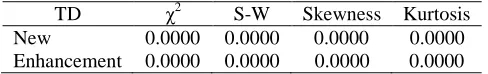
The number of data sets to be compared, data dependence, and data distribution are criteria to select a suitable statistical test. Chi-squared (χ2), Shapiro-Wilk, skewness, and kurtosis statistical tests are performed for data distribution. Table 3 shows the results of these four tests by type of development. Since the smallest p-value amongst the four tests by data set is less than 0.01, the notion that the data comes from a normal distribution can be rejected with 99% confidence for the two types of development.

TD χ2 S-W Skewness Kurtosis

New 0.0000 0.0000 0.0000 0.0000

Enhancement 0.0000 0.0000 0.0000 0.0000

Table 3: P-values for normality tests

Since more than two data sets are compared by type of development (Table 2), they are independent, and data are not normality distributed (Table 3), the suitable statistical test to compare the data sets is Kruskal-Wallis [2], which tests the null hypothesis that the medians within each of the data sets is the same. Since the p-value of Table 4 is greater than 0.01, there is not a statistically significant difference amongst the medians of the data sets at the 99.0% confidence level for the two types of development.

TD p-value

New 0.6748

Enhancement 0.3120

Table 4: Kruskal-Wallis test

As for re-development type, Table 2 includes five data sets of this type; however, all of them have between two and nine projects, therefore, it could not possible to compare any data set for this type.

Second experiment:

Since two data sets are compared (i.e., new and enhancement ones), they are independent, and the data are not normality distributed (Table 3), the suitable statistical test to compare the data sets is Mann-Whitney W [2], which tests the null hypothesis that the medians within each of the two data sets is the same. The DD median values were 12.5 and 22 for new and enhancement projects, respectively. The p-value for this test was equal to 0.0000, thus, there is a statistically significant difference amongst the medians of the two data sets at the 99.0% confidence level.

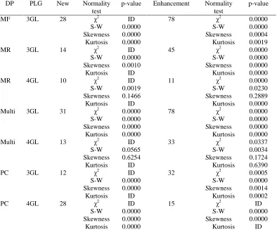
Third experiment:

(6)

DP PLG New Normality test

p-value Enhancement Normality test

p-value

MF 3GL 28 χ2

ID 78 χ2

0.0000

S-W 0.0000 S-W 0.0000

Skewness 0.0000 Skewness 0.0004

Kurtosis 0.0000 Kurtosis 0.0019

MR 3GL 14 χ2 ID 45 χ2 0.0000

S-W 0.0000 S-W 0.0000

Kurtosis ID Kurtosis 0.0000

MR 4GL 10 χ2 ID 11 χ2 0.0000

S-W 0.0019 S-W 0.0230

Multi 3GL 31 χ2 0.0000 78 χ2 0.0000

S-W 0.0000 S-W 0.0000

Kurtosis 0.0000 Kurtosis 0.0000

Multi 4GL 13 χ2 ID 33 χ2 0.0337

S-W 0.0565 S-W 0.0034

PC 3GL 12 χ2 ID 32 χ2 0.0005

S-W 0.0000 S-W 0.0000

PC 4GL 28 χ2 ID 15 χ2 ID

S-W 0.0000 S-W 0.0000

Kurtosis 0.0000 Kurtosis ID

Table 5: Normality statistical tests obtained from data sets of TD by DP and PLG (ID: Insufficient data, S-W: Shapiro-Wilk)

In accordance with Table 6, all medians for new projects are lower than those ones for enhancement projects. Moreover, three of the seven comparisons of Table 6 have statistical difference at 95% of confidence.

DP PLG New Enhancement p-value

NP Median NP Median

MF 3GL 28 10 78 30 0.0133

MR 3GL 14 10 45 25 0.0449

MR 4GL 10 9 11 11 0.5962

Multi 3GL 31 16 78 18 0.6720

Multi 4GL 13 11 33 23 0.0897

PC 3GL 12 11 32 24 0.0500

PC 4GL 28 9 15 18 0.1321

(7)

5 Conclusions

A higher data set size, a better generalization from their data is possible for DD prediction models. A common guideline on software engineering data sets is separate projects in accordance with their attributes such as type of development, development platform, and programming language generation. Data sets of software projects have commonly been used for either analyzing productivity or building prediction models. In this study, defect density of software projects was statistically analyzed to know if there was any difference between projects taking into account the three mentioned attributes.

After the analysis based on statistical significance for the three experiments described in Section 4, the following conclusions can be written from projects developed on platforms and coded in programming languages included in those data sets of Table 2 having ten or more projects:

First experiment:

There is no difference among the DD of new projects.

There is no difference among the DD of enhancement projects. Second experiment:

There is difference between the DD of new and enhancement projects. Third experiment:

There is difference between the DD of new and enhancement projects when developed on MF and coded in 3GL, MR and coded in 3GL, and PC and 3GL.

There is no difference between the DD of new and enhancement projects when developed on MR and coded in 4GL, Multi and coded in 3GL, Multi and coded in 4GL, and PC and 4GL. Based on these results, in a software business scenario, the manager having few data obtained from his own software projects developed on different development platforms and coded in programming language generations can (1) statistically analyze his data sets to conclude if they could be pooled, or (2) use data of the projects used in the present study as a reference, such that the manager generates prediction models or analyzes productivity.

Regarding limitations of this study, the ISBSG Release 2018 data set used has more than eight thousand software projects; however, after applying criteria included in Tables 1 and 2, only 136 new and 341 enhancement software projects could be selected.

Future work will be related to the proposal of models for the new or enhancement software projects analyzed in this study, that is, the models will be trained and tested from the 136 new projects, and from the 341 enhancement projects. Two types of models will be proposed: classifiers and regression models. As for the first one mentioned, the ISBSG Release 2018 classifies the size of projects according their size (measured in function points) in categories such as extra-small, small, medium, large, and extra-large, accordingly, our future work will propose models based on Bidirectional Associative Memories [18], ontologies [19], Alpha-Beta models [20], associative models [21] for classifying projects in accordance with their effectiveness value based on DD. Regarding second type, regression models such as [22] [23] [24] [25] will be applied to predict the DD of new and enhancement projects.

Aknowledgment

(8)

References

[1] P. Bourque and R. Fairley, “Guide to the Software Engineering Body of Knowledge, SWEBOK V3.0”, IEEE Computer Society, 2014.

[2] C. López-Martín, “Predictive Accuracy Comparison between Neural Networks and Statistical Regression for Development Effort of Software Projects”, Applied Soft Computing, Elsevier, vol. 27, 2015, pp. 434-449. DOI: 10.1016/j.asoc.2014.10.033

[3] ISBSG, “Guidelines for use of the ISBSG data, Release 2018”, International Software Benchmarking Standards Group, 2018.

[4] L. Kumar, S.K. Sripada, A. Sureka, S.K. Rath, “Effective fault prediction model developed using Least Square Support Vector Machine (LSSVM)”, The Journal of Systems and Software, Elsevier, vol. 137, 2018, pp. 686–712. DOI: 10.1016/j.jss.2017.04.016

[5] S.S. Rathore and S. Kumar, S., “Towards an ensemble based system for predicting the number of software faults”, Expert Systems With Applications, Elsevier, vol. 82, 2017, pp. 357–382. DOI: 10.1016/j.eswa.2017.04.014

[6] C. López-Martín, M. Azzeh, A. Bou-Nassif, S. Banitaan, “ʋ-SVR Polynomial Kernel for Predicting the Defect Density in New Software Projects”, in Proceedings of the 16th IEEE International Conference on Machine Learning and Applications, 2017. DOI: 10.1109/ICMLA.2017.0-101

[7] I. Myrtveit and E. Stensrud, “Validity and reliability of evaluation procedures in comparative studies of effort prediction models”, Empirical Software Engineering, Springer. Vol. 17, 2017, pp. 23-33. DOI: 10.1007/s10664-011-9183-7

[8] P. Knab, M. Pinzger, B. Bernstein, “Predicting Defect Densities in source code files with Decision Tree Learners”, in Proceedings of the International workshop on Mining software Repositories, 2006. DOI: 10.1145/1137983.1138012

[9] V. Kumar, “Applying soft computing approaches to predict defect density in software product releases: an empirical study”, Computing and Informatics, Vol. 32, 2013, pp. 203-224.

[10] O. Kutlubay, B. Turhan, A.B. Bener, “A Two-Step Model for Defect Density Estimation”, in Proceedings of the 33rd EUROMICRO Conference on Software Engineering and Advanced Applications (EUROMICRO), 2007. DOI: 10.1109/EUROMICRO.2007.13

[11] N. Mandhan, D.K. Verma, S. Kumar, “Analysis of Approach for Predicting Software Defect Density using Static Metrics”, in Proceedings of the IEEE International Conference on Computing, Communication and Automation, 2015. DOI: 10.1109/CCAA.2015.7148499 [12] N. Nagappan and T. Ball, “Use of Relative Code Churn Measures to Predict System Defect

Density”, in Proceedings of27th international conference on Software engineering, 2005, pp. 284–292. DOI: 10.1145/1062455.1062514

[13] C. Rahmani and D. Khazanchi, “A Study on Defect Density of Open source software”, in Proceedings of the 9th International conference on Computer and Information Science, 2010. DOI: 10.1109/ICIS.2010.11

[14] M. Sherriff, N. Nagappan, L. Williams, M. Vouk, “Early Estimation of Defect Density Using an In-Process Haskell Metrics Model”, ACM SIGSOFT Software Engineering Notes, vol. 30, 2005. DOI: 10.1145/1082983.1083285

[15] D. Verma and S. Kumar, “Prediction of defect density for open source software using repository metrics”, Journal of Web Engineering, Rinton, vol. 16, issue 3-4, 2017, pp. 93-310. [16] H.B. Yadav and D.K. Yadav, “A fuzzy logic based approach for phase-wise software defects

prediction using software metrics”, Information and Software Technology, Elsevier, vol. 63, 2015, pp. 44–57. DOI: 10.1016/j.infsof.2015.03.001

(9)

10.1007/s10664-008-9072-x

[18] M.E. Acevedo, C. Yáñez-Márquez, M.A. Acevedo, “Bidirectional Associative Memories: Different Approaches”, ACM Computing Surveys, Association for Computing Machinery, Vol. 45, No. 2, 2013, pp. 1-30. DOI:10.1145/2431211.2431217

[19] S. Cerón-Figueroa, I. López-Yáñez, W. Alhalabi, O. Camacho-Nieto, Y. Villuendas-Rey, M. Aldape-Pérez, C. Yáñez-Márquez, “Instance-based ontology matching for e-learning material using an associative pattern classifier”, Computers in Human Behavior, Elsevier, Vol. 69, 2017, pp. 218-225. DOI:10.1016/j.chb.2016.12.039

[20] López-Yáñez, I., Yáñez-Márquez, Cornelio, Camacho-Nieto, O., Aldape-Pérez, M., Argüelles-Cruz, A.J. (2015). Collaborative learning in postgraduate level courses, Computers in Human Behavior, Elsevier, Vol. 51, Part B, pp. 938-944. DO:10.1016/j.chb.2014.11.055

[21] I. López-Yáñez, L. Sheremetov, C. Yáñez-Márquez, “A Novel Associative Model for Time Series Data Mining”, Pattern Recognition Letters, Elsevier, Vol. 41, 2014, pp. 23-33. DOI:10.1016/j.patrec.2013.11.008

[22] J.A. Antón-Vargas, Y. Villuendas-Rey, C. Yáñez-Márquez, I. López-Yáñez, O. Camacho-Nieto, “Improving the performance of an associative classifier by Gamma Rough Sets based instance selection”, International Journal of Pattern Recognition and Artificial Intelligence, World Scientific, Vol. 32, No. 1, 2018, pp. 1860009. DOI:10.1142/S0218001418600091 [23] A.V. Uriarte-Arcia, C. Yáñez-Márquez, J. Gama, J., I. López-Yáñez, O. Camacho-Nieto,

“Data Stream Classification Based on The Gamma Classifier”, Mathematical Problems in Engineering, Hindawi, Volume 2015, Article 939175, 17 pages. DOI:10.1155/2015/939175 [24] C. Yáñez-Márquez, I. López-Yáñez, M. Aldape-Pérez, O. Camacho-Nieto, Y. Villuendas-Rey,

“Theoretical Foundations for the Alpha-Beta Associative Memories: 10 Years of Derived Extensions, Models, and Applications”, Neural Processing Letters, Springer, Vol. 48, Issue 2, 2018, pp. 811-847. DOI:https://doi.org/10.1007/s11063-017-9768-2