VOLUME 41, ARTICLE 37, PAGES 1059
-
1090
PUBLISHED 22 OCTOBER 2019
http://www.demographic-research.org/Volumes/Vol41/37/ DOI: 10.4054/DemRes.2019.41.37
Research Article
The age difference between spouses and
reproduction in 19
thcentury Sweden
Paul Rotering
Hilde Bras
This publication is part of the Special Collection on “The Power of the Family,” organized by Guest Editors Hilde Bras and Rebecca Sear.
© 2019 Paul Rotering & Hilde Bras.
This open-access work is published under the terms of the Creative Commons Attribution 3.0 Germany (CC BY 3.0 DE), which permits use, reproduction, and distribution in any medium, provided the original author(s) and source are given credit.
1 Introduction 1060
2 Age difference between spouses 1060
2.1 Age difference and female autonomy 1060
2.2 Spousal age difference and fertility: evidence from previous studies 1062
3 Marriage and reproduction in 19th century Sweden 1063
4 Hypotheses 1067
4.1 The ability to have a child 1067
4.2 The nature of the relationship 1067
5 Data, measures, and methods 1068
5.1 Data 1068
5.2 Outcome variables 1069
5.3 Independent variables 1070
5.4 Methods 1073
6 Results 1073
7 Discussion 1080
8 Conclusion 1083
The age difference between spouses and reproduction in 19
thcentury
Sweden
Paul Rotering1
Hilde Bras2
Abstract
BACKGROUND
The influence of spousal relations on reproductive outcomes has received considerable attention in the demographic literature. Previous studies have shown the complex interplay between age difference, female autonomy, and reproductive outcomes, but only a few have focused on historical high-fertility populations.
OBJECTIVE
This study investigates the associations between spousal age difference and the timing of first and higher order births, as well as the total number of children born.
METHODS
Data from the Demographic Data Base (married women, born between 1840 and 1889, first marriages only) are used to construct individual life courses in central and northern Sweden. The relative risk of age-homogamous and age-heterogamous couples having a child is examined using event history analysis. Poisson regression is applied to identify the effects of age difference on the total number of children born.
RESULTS
After controlling for the age of the wife, women in wife-older marriages show higher hazard rates for the transition to first and later order births compared to women in age-homogamous marriages. By contrast, women in husband-older marriages show lower hazard rates for the transition between births, with the exception of first childbirth. However, the net effect of spousal age difference on the total number of children ever born is small.
CONTRIBUTION
This study provides empirical evidence of the association between spousal age gap and fertility outcomes, using the spousal age gap as a proxy for conjugal power. It shows that women in wife-older marriages used their greater female autonomy to shorten the
interval between childbirths, although the effect on the total number of children born is negligible.
1. Introduction
The question of whether female autonomy within marriage is related to fertility outcomes is addressed in a growing body of empirical research, most of which focuses on contemporary high fertility populations such as sub-Saharan African or Asian societies (see Upadhyay et al. 2014 for a recent overview), or contemporary low fertility populations (e.g., Osiewalska 2018). By contrast, the number of studies addressing spousal power differences in historical populations is relatively small (e.g., Feng et al. 2010). Insight into the association between female autonomy and reproductive outcomes can contribute to our understanding of regional variations in the decline of fertility (Casterline, Williams, and McDonald 1986).
In this study, historical parish registration data from central and northern Sweden between 1840 and 1889 are used to examine the association between female autonomy and reproductive outcomes in a historical population. The ability of women to influence reproductive decision-making may depend on their position within the marriage. Spousal age difference is used here as a proxy for female autonomy, reflecting a woman’s bargaining power regarding reproductive decision-making (Abadian 1996; Casterline, Williams, and McDonald 1986; Skinner 1993; Bras and Schumacher 2019). The aim of this study is to examine whether age difference between spouses can explain the timing of first and higher order births, as well as the total number of children born.
The structure of this paper is as follows. The following section provides a brief overview of the literature on the associations between spousal age difference, female autonomy, and reproductive outcomes. There then follows an account of the nature of
Swedish marriages and reproduction during the 19th century. The hypotheses, data, and
methods are presented in the next sections, followed by a discussion of the empirical results and the main conclusions.
2. Age difference between spouses
2.1 Age difference and female autonomy
reproductive decision-making (Abadian 1996; Skinner 1993). In general, a smaller age difference between spouses suggests a higher degree of equality between them. One body of research suggests that industrialization in Western Europe has led to a reduction in patriarchal inequalities within the family, thereby increasing the bargaining power of women (Janssens 2007; Watkins 1993). In a second body of research, fertility transitions are seen as the manifestation of a cultural shift towards egalitarian partnerships. According to Mason (1993), couples who are more socially equal and emotionally intimate face lower costs of family planning, since there is a greater agreement between them on the factors on which the discussion should be based and because there is a greater ability to discuss matters of reproduction. The same line of reasoning is observed in Van de Putte et al. (2009), who argue that the experiences of people belonging to the same birth cohort contribute to a sense of commonality. Shared life experiences and values regarding marriage and family life reinforce and mutually confirm each other’s behavior (Van de Putte et al. 2009: 1236). Van de Putte et al. (2009) observe that the age difference between spouses declined over the course of the
19th century in Western European societies. They argue that the increase in age
homogamy brought with it a more egalitarian view of marriage and partner selection. However, as Pyke and Adams (2010) argue, the husband’s older age does not necessarily mean that all discussions between spouses are dominated by the husband. Nevertheless, from a comparative perspective, a high proportion of marriages in which the husband is older can be seen as indicative of patriarchal family systems in which women’s decision-making power on matters concerning reproduction is constrained (Barbieri, Hertrich, and Madeleine 2005; Cain 1993).
findings illustrate that the effect of women’s empowerment on fertility depends to a large degree on the regional context and the way female empowerment is measured.
2.2 Spousal age difference and fertility: evidence from previous studies
In their study on age difference between spouses in developing regions, Casterline, Williams, and McDonald (1986) identify three mechanisms through which spousal age difference can affect fertility. First, an increase in the age of either spouse is inversely associated with fecundability. A larger age difference will therefore negatively affect reproductive outcomes (Mineau and Trussell 1982). Second, larger age differences are associated with a higher risk of marital dissolution due to widowhood or severe sickness of either the husband or wife. Finally, less palpable but perhaps more substantial effects of large age differences on reproduction can be observed through its effect on variables affecting coital frequency, such as marital stability and satisfaction, preferences concerning family size, and the use of contraception (Barbieri, Hertrich, and Madeleine 2005; Casterline, Williams, and McDonald 1986; Knodel 1988; McDonald 2000). Together, these elements reflect both the direct effects of a higher age of either the wife or the husband on fertility (the ability to have children), and how reproductive decisions depend on the degree of equality between husband and wife (the nature of the relationship).
the mean spousal age difference, the mean age at marriage, and the percentage of female enrolment in secondary education – on total fertility rates in a comparative study of 54 countries in the 1990s. Abadian (1996) finds that, comparing countries, fertility rates are inversely correlated with age at marriage and female education but not with spousal age difference. Barbieri, Hertrich, and Madeleine (2005) examine the effect of spousal age difference, used as a proxy for the degree of equality between spouses, on contraceptive use in eighteen sub-Saharan African countries during the 1990s. They find that couples with small age differences are more likely to use contraceptives than husband-older couples.
An important question is whether women with greater autonomy with respect to their husband use their conjugal power to either enhance or restrict reproductive outcomes, or whether there is no effect whatsoever on fertility outcomes. The empirical literature does not provide a definitive answer to this question. Given that the physical burden of childbearing is higher for women than men, it is arguably in the interest of the wife to postpone the birth of subsequent children or to have fewer children. Women with more authority in the decision-making process regarding having children may therefore be more likely to postpone childbirth. However, evolutionary biology suggests that all individuals face a tradeoff between the costs of reproduction and the benefits of having children in terms of inclusive fitness (Conde-Agudelo, Rosas-Bermúdez, and Kafury-Goeta 2006, 2007; Hamilton 1964a, 1964b; Hrdy 2009; Mace 2014). This suggests that women with greater conjugal power can be more successful in increasing their fertility than women with less conjugal power. An important assumption for the association between conjugal power and fertility outcomes is that husbands’ and wives’ fertility preferences are different. If men’s and women’s fertility preferences are similar, it follows that there is no association between conjugal power and fertility outcomes. As described above, the empirical evidence from the literature is mixed: Some studies find shorter birth intervals for wife-older marriages in some regions (Feng et al. 2010), while others find that husband-older marriages are indicative of shorter birth intervals (Upadhyay et al. 2014).
3. Marriage and reproduction in 19
thcentury Sweden
The demographic transition in Sweden started around 1810, when infant mortality began to steadily decline, followed by a permanent decline in birth rates after the 1870s (Brändström and Sundin 1981; Hofsten and Lundström 1976). Swedish marriages in the
19th century were not only an arrangement between two families but also a social
equal share of property held in common and all children born within wedlock became legal inheritors to their parents. The law also stipulated that no person could be forced
into marriage (Giftermålsbalken: ch. 1:5).3 While parental influence on the choice of
marriage partner was visible through the parents’ involvement in marriage negotiations and their right to disinherit children who married against parental will, Swedish legislation made it possible for marriages to be formed on the basis of romantic love (Ågren 2009; Dribe and Lundh 2014; Lundh 2003; Van de Putte et al. 2009).
The custom of betrothal, or engagement, was deeply rooted in the old Germanic
tradition. With the introduction of Christianity in the early 13th century the ritual was
not dismissed; rather, its role was made more prominent. Betrothal signified the commitment of both partners, as well as their families, to the marriage. The 1734 Marriage Code required that all Christian weddings, the only legal form of marriage, were announced by the publishing of marriage banns, and a betrothal was to precede the wedding. This gave the betrothal legal effects and children of betrothed couples had the same inheritance rights as children born in wedlock. If the fiancé refused to marry after becoming betrothed, the woman maintained her right to her share of the property in the man’s household (Lundh 2003).
Although betrothal affirmed the status of women, an unmarried woman was not autonomous but was under the authority of a male person, usually her father, who acted
as a guardian (giftoman) on her behalf (Giftermålsbalken: ch. 1 par 1.2). Since
unmarried children were considered to belong to the parental household, parents had the right to disinherit children if they married against the parental will, even in the case of remarriage after widowhood (Giftermålsbalken: ch. 6). Parental influence is also visible in the help parents offered in selecting a suitable partner, although parental influence over women was stronger than that over men, who could more easily refuse the involvement of their parents (Dribe and Lundh 2014). Contemporary narrators describe how farmers in particular had a strong influence on their daughter’s partner selection, as they strove to retain the size of the parental homestead. Also, marrying beneath one’s social position was strongly resisted and could result in a couple falling out of favour in the community, or ‘standing outside the village’ (Dribe and Lundh 2014, p. 230). Parents generally sought wealthy partners from within the same social group.
At the time of engagement, the suitor traditionally provided the woman’s guardian
with a gift (vängåva), the value of which was dictated by law. However, by the 19th
century it had become customary to give the gift directly to the bride. If the betrothal agreement was violated, the party not upholding the promise was forced to return the betrothal gifts and to pay a fine to the other family. At marriage, the bride’s parents
provided her with a dowry (medgift), traditionally consisting of a bed, money, or
3 The 1734 Giftermålsbalken, Swedish marriage laws, are available online at https://sv.wikisource.org/
various household goods. The dowry remained the private property of the bride, though
administered by the husband, and reverted to the bride’s family if the marriage ended.4
Apart from her dowry, the wife received a gift from her husband on the day after the
wedding (morgongåva; morning gift), which became the woman’s private property and
was intended to provide her with support in case of widowhood (Ågren 2009; Dribe and Lundh 2014).
Besides the law and the parents, the Church also had a strong influence on premarital relationships in Sweden. Given the relatively small geographical size of the marriage market, the Sunday service in the parish church provided a place for young people to meet in person, as did the local market. Christian morality regarding prenuptial sexual relations was very negative. The Church strongly opposed premarital conception and required the payment of a fine, corresponding to about one month’s pay for a farm hand (Kälvemark 1980: 330). However, the fact that legislation was in place to protect betrothed women and their children if the husband violated the wedding agreement was a clear sign that, in practice, premarital sexual relations were widespread. Farmers in particular appear to have had a pragmatic attitude to premarital intimate relationships – for example, if the harvest or costly wedding preparations forced the marriage to be delayed – as long as the couple married later (Dribe and
Lundh 2014).5 In spite of the prohibition against premarital conception, Kälvemark
(1980) observes that illegitimate births were indeed numerous in southern Sweden, as around 8% to 14.9% of all married women gave birth out of wedlock and around a third of all married couples experienced premarital conceptions.
As in other West European countries, married couples in 19th century Sweden were
expected to establish independent households (Hajnal 1982; Laslett and Wall 1972). The man was expected to have an occupation that could support a family and to have saved enough money to set up a household. Consequently, entry into marriage was fairly restricted, causing a considerable proportion of the population to remain unmarried and resulting in a relatively high age at first marriage. Various arrangements facilitated the acquisition of household goods, a home, and money for the wedding. Access to land or a home could be provided through inheritance from both partners’
parents, given in advance as a wedding gift.6 From 1845, inheritance rights were equal
by law, although in practice one heir could still be favoured by setting a low price on
4 Ågren (2009) describes how the combination of legal and customary practices related to the wife and
husband’s ownership of property, referred to in court documents asarcanum domesticum, could make it difficult for creditors to assess the size of their debtors’ assets (Ågren 2009:13‒16, 146‒147).
5 Still, rural society was intolerant towards unmarried mothers and their illegitimate children and regarded
pregnant brides as a disgrace (Dribe and Lundh 2014).
6 Such decisions on the transmission of property not only concerned the formation of a new household with
the property, giving him or her the advantage to buy out the other siblings on favourable
terms (Ågren 2009: 189‒190; Lundh 2003: 14). Relatives, friends, and wedding guests
also helped to set up the household, as it was customary to bring household goods as gifts for the newlywed couple. Relatives who lived further away and could not attend the wedding usually sent money. Lundh (2003) argues that the institution of wedding gifts in central and northern Sweden played a prominent role in affirming social relations, as the names of the givers and the value of the gift were announced in public during the wedding. Reciprocity was another important aspect of the wedding gifts: those who received support were obliged to return the favour if needed (Lundh 2003), making communal cooperation an important aspect of the wedding. Guests were also expected to contribute to the wedding feast by bringing food and drink. These arrangements relieved the financial burden of the wedding for the betrothed couple.
During the 19th century the legal minimum marriage age in Sweden was increased
from 15 to 17 years for women and from 20 to 21 years for men (Lundh 2003: 41).7
Over the entire course of this study, in the regions of Sundsvall and Skellefteå the actual
average age at marriage was around 25 years for women and 27.5 years for men.8
Although Swedes married relatively late, these ages are similar to those in other North Western European countries (Hajnal 1982).
Altogether, Swedish marriages in the 19th century were characterized by
considerable equality between the spouses. The homogamous nature of the marriage was reflected in various elements of the marital union. A betrothed woman and her illegitimate children were protected in case the man did not comply with the betrothal agreement. By law, the husband could only be married to one wife at a time. Furthermore, in the rare case of divorce the wife had a right to half the property held in common. From the Civil Code of 1734 up until 1915, the legally recognized reasons for divorce were abandonment and adultery, although divorce was opposed by the Church
and socially frowned upon (Lundh 2003: 11‒12). The homogamous nature of marriage
was also reflected in the selection of partners. Although parents could influence the
choice of partner, in the 19th century young people were increasingly able to express
their own preferences due to the rise of wage labour and increase in the landless population. The relatively small age difference between spouses clearly indicates the
7 The 1734 law determined a minimum age of 15 years for women and 20 for men. In 1920 the minimum
marriage age was set at 18 years for both men and women. Sverikes rikes lag, Giftermålsbalken 1920: Ch 2 and 1:https://www.riksdagen.se/sv/Dokument-Lagar/Lagar/Svenskforfattningssamling/Giftermalsbalk-19204 05_sfs-1920-405/?bet=1920:405 (last visit: July 10th, 2017)
8 Calculated for the data used in this paper. Between 1840 and 1870 the marriage age for women declined
egalitarian nature of 19th century Swedish marriages compared to those in other societies (Cain 1993).
4. Hypotheses
Following Casterline, Williams, and McDonald (1986), spousal age difference can indicate the nature of a relationship and the ability to have children. These two aspects facilitate the development of the hypotheses formulated below. It is important to recognize that fertility outcomes depend on a multitude of factors, including socioeconomic conditions, customs or other cultural aspects, and the age of both the husband and the wife. These factors are all assumed to be constant in the formulation of the hypotheses.
4.1 The ability to have a child
The existence of a spousal age gap by default entails that one spouse is older and therefore has a higher risk of mortality or infecundity. The wife’s age is the most important factor influencing her ability to have a child (Bongaarts and Potter 1983; Wilson, Oeppen, and Pardoe 1988), although the chance of having a child also decreases when her husband becomes old and is more likely to become ill or pass away. Furthermore, other non-physiological factors such as marital satisfaction and sexuality may be inversely correlated with age (Casterline, Williams, and McDonald 1986). Thus, ceteris paribus, a larger age gap between husband and wife reduces their
likelihood of having children. Therefore:For a given age, women in age-homogamous
marriages are more likely to enter parenthood, to have shorter birth intervals, and to have a larger number of children ever born than women (of similar age) in husband-older relationships (H1).
4.2 The nature of the relationship
Age difference can lead to a fertility outcome that is more beneficial to the older partner if he or she is better able to influence decisions regarding reproduction. The assumptions here are that age differences reflect the older partner’s autonomy, that fertility preferences differ between partners, and that a wife with greater conjugal power strives to increase her fertility. Controlling for the wife’s age and other characteristics,
wife-older couples and longer for husband-older couples, compared to same-age couples. Furthermore, wife-older couples are likely to have more children and husband-older couples are likely to have fewer children compared to same-aged couples (H2a).
Alternatively, assuming women with greater conjugal power strive to reduce
fertility in order to reduce the biological costs of pregnancy:For women of similar age,
women in wife-older couples will enter parenthood later and have longer birth intervals and fewer children than same-aged and husband-older couples (H2b).
5. Data, measures, and methods
5.1 Data
The data used in the analysis are obtained from the POPUM and POPLINK databases
of the Demographic Data Base (DDB).9 The DDB is a large, historical population
database containing linked individual-level records from Swedish parish registers. The parish records contain event registrations such as births, baptisms, banns, marriages, deaths, and migration (Alm-Stenflo 1994; Jeub 1993). Parish registration has been regulated by canon law since 1686, but there has been variation in the way events are
registered. The establishment of the Statistical Commission (Tabellverket) in 1749 and
the introduction of printed forms in the 1780s led to uniform methods of population registration. The DDB has digitized the registers of a select number of parishes, allowing for the construction of the individual life histories of the people living in these parishes.
An important advantage of the DDB for this study is that it is possible to follow individuals over the life course for as long as they remained in a parish registered in the DDB. Event registrations such as date and place of birth, marital status, sex, and occupation are available for each individual, as well as their relationship to other family members. Furthermore, the DDB data include information on the exact period during which a person is observed. While the quality of the DDB is high and the number of registered people in the database is large, there are some limitations to its use. First, the digitization of parish registration is incomplete. This means that information on people moving to neighbouring parishes can be lost when that parish is not available in the database, and so not everybody can be followed throughout their entire life. However, information up to the moment of out-migration can be used. Second, the records were maintained by the parish clergy, whose task was to continuously update the birth and
9 DDB: Demographic Data Base. Centre for Demographic and Ageing Research (CEDAR), Umeå University.
baptismal registers, registers of banns and marriages, registers of deaths and burials, migration lists and catechetical lists (including details about church attendance and knowledge of the scriptures). In fast-growing parishes or municipalities where servants, soldiers, or lodgers frequently moved in and out of the parish, it was difficult for the parson to record the required information. In addition, there are gaps due to the quality of the handwriting, the past treatment of the registers, and the occurrence of accidents, so not all material could be preserved and digitized (Jeub 1993).
This study is based on the life histories of 8,258 women born between 1840 and 1890 in the regions of Sundsvall and Skellefteå in central and northern Sweden. The following criteria were set for the inclusion of a woman in the analysis: She was born in the area of Sundsvall or Skellefteå, or entered a parish in this region at the age of 18 years or younger; she was married at least once; and the parish registration includes information on the occupation of her husband. The sample size for the analysis of completed fertility is smaller than that for parity transition due to migration to an unknown parish, marriage dissolution, the death of either the wife or the husband, or clerical error. Complete information is available for 6,235 women. This means that they did not migrate to an unknown parish before the age of 45, and that both wife and husband survived until age 45. The construction of the sample emphasizes the observation of a woman’s complete birth history. This gives the sample a bias towards people who did not migrate to a parish not registered in the DDB. Given the institution of domestic service, the life histories of many people are truncated. As can be seen in the description of the data below, a large share of the population in this sample
belonged to the farmer class, while during the second half of the 19th century Swedish
society as a whole witnessed industrialization and an increase in the landless labouring class.
5.2 Outcome variables
analysis, second or later marriages of both wife and husband are excluded. The outcome variables are the woman’s age at first birth, the duration of the interval between subsequent births, and the total number of children born. The birth interval is a useful indicator of fertility and is frequently used in the literature on reproduction (see, e.g., Feng et al. 2010; Van Bavel and Kok 2004, 2010; Van Poppel et al. 2012).
5.3 Independent variables
The main independent variable in this analysis is age difference between spouses. The age difference is included here using dummy variables, where the reference category is an age difference between spouses of at most two years. An age difference of more than two years is coded separately for wife-older marriages and husband-older marriages. The definition of same-age marriages as marriages where the age difference between spouses is at most two years is also used in Van de Putte et al. (2009). By contrast, Feng et al. (2010) consider marriages where the husband is zero to five years older as age homogamous. In the present study the use of other ranges did not influence the outcomes of the analysis to any great extent.
Table 1 provides descriptive information on the different variables used in the models. The husband is older than the wife in around half of all couples. Wife-older marriages are less frequently observed and their share decreased over time from around 22% to around 14% of all marriages. In contrast to Van de Putte et al. (2009), the data in this sample do not indicate an increase in age homogamy over time. This is presumably due to the selection of couples of which the majority belong to the farmer class and that display regional immobility.
In order to control for changes in socioeconomic or cultural conditions and fertility over time, dummy variables are included for the birth cohort of the wife. Community-level characteristics are controlled for using a dummy variable for the region where the wife is born. Two regions are selected based on the quality and availability of data: Sundsvall, near the Gulf of Bothnia around 400 kilometres north of Stockholm, and Skellefteå, which is located along the same coast around 350 kilometres north of
Sundsvall. Forestry was the main economic activity in the first half of the 19th century
in both Skellefteå and Sundsvall, while in Sundsvall agriculture also played an important role. The towns were small and population density was low compared to towns in other European countries. From the 1850s, industrialization and international trade spurred economic growth, particularly in the Sundsvall region, and encouraged the development of shipyards and iron foundries (Alm-Stenflo 1994; Schön 1997).
as HISCO codes, which are converted to the HISCLASS classification scheme. The HISCLASS scheme allows for a systematic comparison of social positions based on occupational titles (Van Leeuwen and Maas 2011; Van Leeuwen, Maas, and Miles 2004). The combination of smaller groups produces four broad social classes, which are included as dummy control variables and are coded as follows: (1) foremen to higher occupations (non-manual labour), (2) farmers, (3) medium- and lower-skilled workers, and (4) lower-manual or unskilled (farm) workers. As Table 1 shows, most couples in the sample belonged to the farmer class (N = 4.506, or 54.6%), followed by medium-and lower-skilled workers.
Individual-level differences in past reproductive outcomes are controlled for by the inclusion of dummy variables for the occurrence of multiple births and the death of the previous child. Previous multiple births may serve as an exogenous factor influencing the time to conception of the next child, given the extra care required to nurture two or more children compared to one. A twin birth increases the birth order of the following child by two instead of one, so if a woman had twins at first childbirth the subsequent childbirth is registered as the third parity. The death of a child before or after eight months, both before the birth of the next child, is coded separately using time-varying dummy variables. The death of a previous child may induce a replacement effect and may thus shorten the time to conception of the next child (Derosas 2006; Knodel 1982; Van Bavel and Kok 2004, 2010). Because breastfeeding can delay the return to ovulation, the child’s survival decreases to a certain degree the woman’s chance of becoming pregnant again (Gray et al. 1990; Santow 1987).
Table 1: Descriptive statistics
Wife +2 years older
Same age (‒2 up to 2 years)
Husband
+2 years older Total
Observations1 1,413 (17.1%) 2,467 (29.9%) 4,378 (53.0%) 8,258 Birth cohort
1840‒1849 (N) 396 (22.2%) 562 (31.5%) 827 (46.3%) 1,785
1850‒1859 (N) 433 (19.5%) 694 (31.2%) 1,095 (49.3%) 2,222
1860‒1869 (N) 279 (13.1%) 615 (29.0%) 1,230 (57.9%) 2,124
1870‒1879 (N) 172 (14.2%) 315 (25.9%) 728 (59.9%) 1,215
1880‒1889 (N) 133 (14.6%) 281 (30.8%) 498 (54.6%) 912
Region
Sundsvall (N) 514 (15.4%) 1,004 (30.1%) 1,823 (54.6%) 3,341
Skellefteå (N) 899 (18.3%) 1,463 (29.8%) 2,555 (52.0%) 4,917
Social class
Foremen to higher (N) 144 (18.5%) 218 (27.9%) 418 (53.6%) 780
Farmer (N) 675 (15.0%) 1,298 (28.8%) 2,533 (56.2%) 4,506
Medium- and lower-skilled (N) 530 (21.4%) 824 (33.3%) 1,124 (45.4%) 2,478
Lower-manual and unskilled farm worker (N)
64 (13.0%) 127 (25.7%) 303 (61.3%) 494
Age of wife
Age at first marriage5 29.4 (3.8) 25.4 (3.3) 23.2 (3.7) 24.9 (4.3) Age at first birth 29.8 (4.1) 26.0 (3.6) 23.9 (3.8) 25.5 (4.4)
Age at last birth2 39.0 (5.0) 38.12 (5.6) 36.59 (6.2) 37.4 (5.9) Age of husband
Age at first marriage 24.6 (3.1) 25.6 (3.3) 29.5 (4.8) 27.5 (4.6)
Age at first birth 25.0 (3.6) 26.2 (3.5) 30.1 (4.9) 28.1 (4.9)
Age at last birth2 34.2 (5.2) 38.3 (5.6) 43.1 (6.8) 40.2 (7.1)
Children ever born
Overall mean 4.9 (2.6) 6.0 (3.0) 6.1 (3.2) 5.9 (3.1)
Mean Sundsvall 4.0 (2.3) 4.8 (2.9) 4.9 (3.1) 4.8 (3.0)
Mean Skellefteå 5.2 (2.6) 6.3 (3.0) 6.5 (3.2) 6.2 (3.1)
Previous child3
Twins 1.36% 1.22% 1.36% 1.32%
Previous child died within eight
months4 7.36% 7.94% 8.08% 7.93%
Previous child died after eight months4
2.87% 3.15% 3.20% 3.14%
Source: DDB, see text. (CEDAR). POPLINK and POPUM version 4.4.2.
Notes:1) Number of observations. Based on sample of all women in the sample (row percentages between parentheses, N=8,258). 2) Based on a sample of women with complete life-course information (N = 6,235).
5.4 Methods
The analysis of the effect of spousal age difference on reproductive outcomes is split into two parts. First, Cox proportional hazard models are fitted to examine whether women’s age at first birth and the likelihood of parity transition are associated with the spousal age gap. The chance of a birth occurring, given a particular age difference between the spouses, is expressed as a coefficient that denotes the hazard of having a child over time relative to an unspecified baseline hazard (Cleves et al. 2010). The assumption of proportionality is examined using Schoenfeld residuals and all models are stratified on the birth cohort of the wife. Each parity transition is estimated separately and control variables are included for the effect of the wife’s age, social status, regional differences, and the occurrence of multiple births or child deaths since last birth. Each parity transition sample includes women who do not have a next childbirth. Birth intervals of more than seven years are excluded from the analysis of each parity transition (N = 280). Analysis time is defined in years, with the woman’s birthdate as the onset of risk of first birth, and the date of previous birth for each subsequent birth. The death of previous children is included as a time-varying covariate, changing the value of the dummy and creating a new episode when the previous child dies.
Second, the association between the total number of childbirths and the spousal age gap is examined using Poisson regression. The baseline model includes controls for social status, regional differences, and temporal variations. The effects of the wife’s age at marriage on the total number of children born are examined in a separate model.
6. Results
of all births occurred after nine months of marriage. As discussed above, the general attitude towards premarital sexual behaviour was contradictory: Christian morality opposed such relations, while legislation strengthened the position of pregnant women during betrothal.
Table 2: Timing of childbirth in the Sundsvall and Skellefteå regions (Sweden), 1840‒1890
Birth cohort wife
1840‒ 1850‒ 1860‒ 1870‒ 1880‒ All
Mean age wife at first birtha
26.4 25.7 24.8 25.0 25.8 25.5
Mean age wife at marriage 25.8 25.2 24.2 23.8 24.9 24.9
Birth interval by parityb
1‒2 26.71 26.13 24.61 23.75 22.67 25.10
2‒3 30.92 29.79 28.38 26.99 25.43 28.79
3‒4 30.95 30.7 28.33 27.88 25.69 29.25
4‒5 31.02 31.01 28.39 29.07 26.19 29.65
5‒6 31.13 29.96 28.44 29.07 26.82 29.51
Mean number of children bornc
5.7 6.1 6.4 6.0 3.8 5.9
Timing of first child
Before the wedding 12.3 % 9.9 % 9.8 % 7.3 % 6.7 % 9.6 %
0‒8 months after the wedding 35.6 % 37.8 % 42.1 % 40.7 % 36.4 % 38.8 %
>8 months after the wedding 52.1 % 52.4 % 48.0 % 52.0 % 56.9 % 51.7 %
Source: DDB (CEDAR). POPLINK and POPUM version 4.4.2. Notes:a) Age in years
b) Birth-to-birth interval in months
c) Women observed age 18‒45 or death before age 45.
Figure 1: Average age at first and last birth in Sundsvall and Skellefteå (Sweden), 1840‒1890, by spousal age difference
Source: DDB, see text. (CEDAR). POPLINK and POPUM version 4.4.2.
Note: The upper three lines show the average age of women at last childbirth; the bottom three lines show the average age of women at first childbirth (N = 6.235).
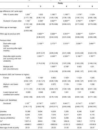
Table 3: Hazard ratios for spousal age differences on the transition time to first and higher order births (Cox regression model)
Parity
1 2 3 4 5 6
Age difference (ref: same age)
Wife +2 years older 1.263*** 1.023 1.180*** 1.190*** 1.178** 1.120+ [1.17,1.36] [0.95,1.10] [1.09,1.28] [1.09,1.30] [1.06,1.31] [0.99,1.26]
Husband +2 years older 1.160*** 0.938* 0.827*** 0.850*** 0.763*** 0.788*** [1.10,1.22] [0.89,0.99] [0.78,0.88] [0.80,0.91] [0.71,0.82] [0.73,0.85]
Wife's age at marriage 0.656*** [0.65,0.66]
Wife's age at previous birth 0.963*** 0.928*** 0.914*** 0.892*** 0.874***
[0.96,0.97] [0.92,0.93] [0.91,0.92] [0.88,0.90] [0.86,0.88]
Previous infant
Died within eight months
(ref: surviving after eight months)
3.109*** 3.173*** 3.319*** 3.836*** 3.654***
[2.87,3.37] [2.89,3.48] [3.01,3.66] [3.43,4.29] [3.22,4.15]
Died after eight months (ref: surviving until next childbirth)
2.001*** 2.039*** 2.259*** 2.160*** 1.787***
[1.74,2.30] [1.78,2.33] [1.97,2.59] [1.83,2.55] [1.49,2.14]
Multiple birth (ref: one child born)
1.638*** 0.748* 0.933 0.81
[1.30,2.06] [0.59,0.95] [0.68,1.27] [0.63,1.05]
Husband's SES (ref: foremen to higher)
Farmer 0.992 1.108* 0.963 1.105+ 1.123+ 1.045
[0.92,1.07] [1.02,1.21] [0.88,1.06] [0.99,1.23] [0.99,1.27] [0.90,1.21]
Medium- and lower-skilled
1.203*** 1.092+ 0.972 1.118+ 1.124+ 1.056
[1.11,1.31] [1.00,1.20] [0.88,1.07] [1.00,1.25] [0.99,1.28] [0.91,1.23]
Lower-manual and unskilled farm worker
0.928 0.946 0.901 1.041 1.01 0.962
[0.82,1.05] [0.83,1.07] [0.78,1.04] [0.89,1.22] [0.84,1.22] [0.77,1.20]
Region (ref: Skellefteå)
Sundsvall 1.107*** 0.716*** 0.670*** 0.641*** 0.714*** 0.739*** [1.05,1.17] [0.68,0.76] [0.63,0.71] [0.60,0.69] [0.66,0.77] [0.68,0.81]
Episodes 15,389 9,634 8,229 7,293 6,246 5,397
Subjects at risk 8,245 7,974 7,016 6,017 4,974 4,110
Failures (childbirths) 7,971 7,003 6,010 5,008 4,062 3,229
Chi2 11671.4 938.8 1156 1252.8 1235.1 1177.9
Log likelihood ‒45688.3 ‒45650.1 ‒38503.6 ‒31351.5 ‒24654.3 ‒19109.9
Table 3: (Continued)
Parity
1 2 3 4 5 6
Number of twin births (at previous parity)
79 72 43 63
Number of children death within eight months
740 556 498 382 303
Number of children death after eight months
212 233 231 160 133
Notes: Stratified by wife's birth cohort.
Transition from wife’s birth to first parity, and between subsequent childbirths. Exponentiated coefficients (hazard ratios). 95% confidence intervals in brackets. + p < 0.10, * p < 0.05, ** p < 0.01, *** p < 0.001.
The results indicate that, controlled for age at marriage, the hazard of a first childbirth (column 1) is higher for both wife-older and husband-older couples compared to same-age couples. Given a particular age at marriage, women who were at least two years older or younger than their husband had their first child at a lower age compared to women in age-homogamous couples. In other words, age-homogamous couples were more likely to delay the birth of the first child. As expected, age at marriage itself is positively associated with age at first birth, meaning that women who married later were having their first child at a higher age. Few social class differences are apparent, except for an increased likelihood of first childbirth for couples where the husband had a medium- or lower-skilled occupation compared to the reference group of foremen and higher occupations. The hazard ratio for the birth of the first child was higher in the economically and industrially more developed region of Sundsvall than in rural Skellefteå.
Looking at the parity transition rates from first to second birth (column 2), second to third birth (column 3), etc., it can be observed that the likelihood of a subsequent birth is higher in wife-older marriages and lower in husband-older marriages compared to age-homogamous marriages. This finding is robust to other specifications of age
difference (e.g., 0‒5 years as reference). The results are significant for all parity
pregnant only once before the birth of the third child. By contrast, the occurrence of multiple births significantly reduced the likelihood of transitioning to the fourth parity, either because raising multiple young children required considerable energy from the parents, causing the delay of the next birth, or because the parents stopped having children altogether. For higher order parities the occurrence of multiple births has no significant effect. Similar to the transition to first birth, there are only small differences between social groups regarding parity transition. Farmers and medium- or lower-skilled workers seem to have had higher hazards of parity transition for some birth intervals compared to couples where the husband was a foreman or higher, but with no clear pattern. Comparing regions, the birth interval was longer for women living in Sundsvall than in Skellefteå.
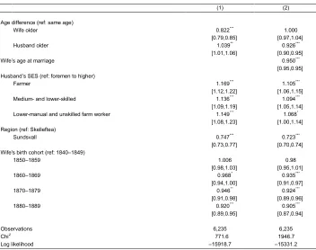
Table 4 provides the results of two Poisson regression models for the association between spousal age difference and the total number of childbirths for all women observed from age 18 until age 45. Both model 1 and 2 include control variables for socioeconomic status, regional differences, and cohort effects. In the second model the wife’s age at marriage is included as an additional control variable. As in Table 3, a regression coefficient greater than 1 denotes a positive association between the number of children born and the independent variable, while a coefficient smaller than 1 indicates a negative association.
Table 4: Effect of spousal age difference on children ever born (Poisson model)
(1) (2)
Age difference (ref: same age)
Wife older 0.822*** 1.000
[0.79,0.85] [0.97,1.04]
Husband older 1.039** 0.926***
[1.01,1.06] [0.90,0.95]
Wife’s age at marriage 0.950***
[0.95,0.95] Husband’s SES (ref: foremen to higher)
Farmer 1.169*** 1.105***
[1.12,1.22] [1.06,1.15]
Medium- and lower-skilled 1.136*** 1.094***
[1.09,1.19] [1.05,1.14] Lower-manual and unskilled farm worker 1.149*** 1.068*
[1.08,1.23] [1.00,1.14] Region (ref: Skelleftea)
Sundsvall 0.747*** 0.723***
[0.73,0.77] [0.70,0.74] Wife's birth cohort (ref: 1840‒1849)
1850‒1859 1.006 0.98
[0.98,1.03] [0.95,1.01]
1860‒1869 0.968* 0.935***
[0.94,1.00] [0.91,0.97]
1870‒1879 0.946** 0.924***
[0.91,0.98] [0.89,0.96]
1880‒1889 0.920*** 0.905***
[0.89,0.95] [0.87,0.94]
Observations 6,235 6,235
Chi2 771.6 1946.7
Log likelihood ‒15918.7 ‒15331.2
Notes: Poisson regression of children ever born to women followed age 18 to 45. Exponentiated coefficients; 95% confidence intervals in brackets.
+ p < 0.10, * p < 0.05, ** p < 0.01, *** p < 0.001.
The results from Table 4 show that after controlling for the age of the wife at marriage, the effects of spousal age gap on the total number of children born are fairly small, with a coefficient of 0.926 for husband-older marriages. In order to further illustrate the limited impact of spousal age difference on the number of children ever born, the total number of childbirths is set graphically against the age of the wife at marriage (Figure 2). It is clear from this figure that women who married at a higher age had fewer children than those who married young. However, as Figure 2 shows, it is hard to identify stark differences between age-heterogeneous and age-homogamous couples in the total number of children ever born.
Figure 2: Average number of children ever born in Sundsvall and Skellefteå (Sweden), 1840‒1890, by spousal age difference and age at marriage
Source: DDB (CEDAR). POPLINK and POPUM version 4.4.2.
Note: Number of children ever born calculated for women followed age 18‒45 (N = 6,235).
7. Discussion
findings, the absolute age of the woman at marriage or previous birth is an important factor influencing the fertility outcomes of the couple, as a higher absolute age reduces the likelihood of transitioning to next childbirth. Table 1 shows that, on average, women in wife-older marriages have a higher age at first marriage than women in husband-older marriages. Women in wife-older marriages also have fewer children and on average start having children at the relatively late age of around 30 years compared to women in husband-older marriages, who on average have their first child at the age of 24. Given that, on average, women in wife-older marriages start later but stop at more or less the same age (see Figure 1), they also have a shorter ‘window’ to have
children before reaching menopause.10 Table 3 confirms that birth intervals are shorter
for women in wife-older marriages compared to same-age or husband-older marriages after controlling for the woman’s age. These findings show that a higher absolute age of women at marriage or previous childbirth reduces the hazard of first and subsequent births, and reduces the total number of children ever born.
Since all analyses include the age of the wife as a control variable, it is possible and perhaps more interesting to consider the relative effects of spousal age difference on fertility outcomes, working not through fecundity but through differences in conjugal power. The results support Hypothesis 2a, showing that after controlling for the age of the woman, women in wife-older marriages have shorter birth intervals. This finding is similar to that observed by Feng et al. (2010) for southern Sweden. Furthermore, in husband-older marriages birth intervals are longer for higher parities and fewer children are born over the life course of each woman. These findings suggest that greater female autonomy, expressed by the spousal age gap, significantly affects fertility outcomes. After controlling for their age, women in wife-older marriages are able to shorten their birth intervals compared to women of similar age in age-homogamous or husband-older marriages. Hypothesis 1 does not find support in our analysis, as age-homogamous couples do not stand out as early starters with short birth intervals and a relatively large number of children ever born.
Some of the results presented above warrant further attention. The likelihood of first childbirth is higher not only for wife-older marriages but also for husband-older marriages. This shows that within husband-older marriages there is a ‘catch-up’ effect as the older husband is likely to encourage the birth of a first child. Furthermore, while women in husband-older marriages have slightly fewer children ever born, women in wife-older marriages do not have significantly more children than age-homogamous couples. The lower number of childbirths observed for women in husband-older marriages may suggest that either the fecundity of men decreases as they become older, thereby reducing their biological ability to have children, or that reduced marital
satisfaction in husband-older marriages reduces fertility outcomes (Casterline, Williams, and McDonald 1986).
8. Conclusion
This study uses historical parish registration data from central and northern Sweden on women born between 1840 and 1889 to examine the associations between conjugal power and various measures of reproductive outcomes. Spousal age gap is used as an indicator of conjugal power (Skinner 1993). The results show that after controlling for age at marriage, women in wife-older marriages, having greater conjugal power, display shorter birth intervals compared to women in age-homogamous marriages. Women in husband-older marriages transition to first birth more quickly than women in age-homogamous marriages, indicating a catch-up effect. By contrast, the likelihood of transitioning to second or higher-order parity is lower in husband-older marriages, suggesting that the lower female bargaining power in such marriages is associated with lower fertility outcomes. The overall effect on the number of children ever born is highly dependent on the absolute age of the woman at marriage. Nevertheless, when the absolute age is controlled for, the results show that women in husband-older marriages had slightly fewer children overall.
The main contribution of this study is that it suggests that when examining fertility outcomes, conjugal power can be approximated using the spousal age gap. However, this study also highlights that the effects of the absolute age of the wife have to be carefully accounted for. Women in wife-older marriages display a preference for shorter birth intervals and a faster transition to first birth. This suggests that while women face considerable costs of reproduction, having children yields a positive inclusive fitness benefit (Conde-Agudelo et al. 2006, 2007; Hamilton 1964a, 1964b; Hrdy 2009; Mace 2014). Vice versa, although the biological costs of having children are lower for men, they do not employ their greater bargaining power within marriage in order to shorten the transition time between births, with the exception of the transition to first birth. By contrast, after the first parity the birth interval is longer in husband-older marriages and the total number of children ever born is slightly lower.
Further research is needed in order to more closely examine the association between female autonomy and reproductive outcomes. Owing to the nature of the available historical data, it is difficult to examine other operationalizations of female autonomy. Other studies show that more-autonomous women are able to delay subsequent births, and thus played an important part in the fertility decline (e.g., Bras and Schumacher 2019). Also, there is no evidence of an increase in age homogamy for the sample used in this study (c.f. Van de Putte et al. 2009). If we were able to extend the time period of our study it would be interesting to see whether our findings remain robust after the population completed the fertility transition. In actuality, fertility outcomes were determined by the specific historical, social, and economic context in
References
Abadian, S. (1996). Women’s autonomy and its impact on fertility.World Development
24(12): 1793‒1809.doi:10.1016/S0305-750X(96)00075-7.
Ågren, M. (2009). Domestic secrets: Women and property in Sweden, 1600‒1857.
Chapel Hill: University of North Carolina Press. doi:10.5149/97808078984
51_agren.
Alm-Stenflo, G. (1994). Demographic description of the Skellefteå and Sundsvall
regions during the 19th century. Umeå: Demographic DataBase, Umeå
University.
Barbieri, M., Hertrich, V., and Madeleine, G. (2005). Age difference between spouses
and contraceptive practice in sub-Saharan Africa.Population (English Edition),
60(5/6): 617‒654.doi:10.2307/4148187.
Bongaarts, J. and Potter, R.E. (1983).Fertility, biology, and behavior: An analysis of
the proximate determinants. New York: Academic Press.doi:10.2307/1973328.
Borgerhoff Mulder, M. (2000). Optimizing offspring: the quantity‒quality tradeoff in
agropastoral Kipsigis. Evolution and Human Behavior 21(6): 391‒410.
doi:10.1016/S1090-5138(00)00054-4.
Borgerhoff Mulder, M. (2007). Hamilton’s rule and kin competition: The Kipsigis case. Evolution and Human Behavior 28(5): 299‒312. doi:10.1016/j.evolhumbehav. 2007.05.009.
Brändström, A. and Sundin, J. (1981). Infant mortality in a changing society. The
effects of child care in a Swedish parish 1820‒1894. In: Brändström, A. and
Sundin, J. (eds.). Tradition and transition: Studies in microdemography and
social change. Umeå: University of Umeå: 67‒104.
Bras, H. and Schumacher, R. (2019). Changing gender relations, declining fertility? An
analysis of childbearing trajectories in 19th-century Netherlands. Demographic
Research 41(30): 873–912.doi:10.4054/DemRes.2019.41.30.
Cain, M. (1993). Patriarchal structure and demographic change. In: Frederici, N.,
Mason, K.O., and Sogner, S.e. (eds.). Women’s position and demographic
change. Oxford: Clarendon Press: 43‒60.
Casterline, J.B., Williams, L., and McDonald, P. (1986). The age difference between
spouses: Variations among developing countries.Population Studies 40(3): 353‒
Cleves, M., Gutierrez, R., Gould, W., and Marchenko, Y. (2010). An introduction to survival analysis using Stata (3rd edition) College Station, TX: Stata Press. Conde-Agudelo, A., Rosas-Bermúdez, A., and Kafury-Goeta, A. (2006). Birth spacing
and risk of adverse perinatal outcomes: A meta-analysis.JAMA 295(15): 1809‒
1823.doi:10.1001/jama.295.15.1809.
Conde-Agudelo, A., Rosas-Bermúdez, A., and Kafury-Goeta, A. (2007). Effects of
birth spacing on maternal health: a systematic review. American Journal of
Obstetrics and Gynecology196(4): 297‒308.doi:10.1016/j.ajog.2006.05.055. Derosas, R. (2006). Between identity and assimilation: Jewish fertility in
nineteenth-century Venice. In: Derosas, R. and Van Poppel, F. (eds.). Religion and the
decline of fertility in the Western World. Cham: Springer: 177‒206.
doi:10.1007/1-4020-5190-5.
Dribe, M. and Lundh, C. (2005). Gender aspects of inheritance strategies and land
transmission in rural Scania, Sweden, 1720–1840. The History of the Family
10(3): 293‒308.doi:10.1016/j.hisfam.2005.03.005.
Dribe, M. and Lundh, C. (2014). Social norms and human agency: Marriage in
nineteenth-century Sweden. In: Lundh, C. and Kurosu, S. (eds.). Similarity in
difference: Marriage in Europe and Asia 1700‒1900. Cambridge: MIT Press: 211‒260.doi:10.7551/mitpress/9780262027946.003.0007.
Feldman, B.S., Zaslavsky, A.M., Ezzati, M., Peterson, K.E., and Mitchell, M. (2009). Contraceptive use, birth spacing, and autonomy: An analysis of the
Oportunidades Program in rural Mexico.Studies in Family Planning 40(1): 51‒
62.doi:10.1111/j.1728-4465.2009.00186.x.
Feng, W., Lee, J.Z., Tsuya, N.O., and Kurosu, S. (2010). Household organization, co-resident kin, and reproduction. In: Tsuya, N.O., Feng, W., Alter, G., and Lee,
J.Z. (eds.). Prudence and pressure, reproduction and human agency in Europe
and Asia, 1700‒1900. Cambridge: MIT Press: 67‒96.
Fricke, T. and Teachman, J.D. (1993). Writing the names: Marriage style, living
arrangements, and first birth interval in a Nepali society. Demography 30(2):
175‒188.doi:10.2307/2061836.
Gray, R.H., Campbell, O.M., Apelo, R., Eslami, S.S., Zacur, H., Ramos, R.M., and
Labbok, M.H. (1990). Risk of ovulation during lactation.The Lancet335(8680):
Hajnal, J. (1982). Two kinds of preindustrial household formation systems.Population and Development Review 8(3): 449‒494.doi:10.2307/1972376.
Hamilton, W.D. (1964a). The genetical evolution of social behaviour. I. Journal of
Theoretical Biology 7(1): 1‒16.doi:10.1016/0022-5193(64)90038-4.
Hamilton, W.D. (1964b). The genetical evolution of social behaviour. II. Journal of
Theoretical Biology7(1): 17‒52.doi:10.1016/0022-5193(64)90039-6.
Hofsten, E. and Lundström, H. (1976).Swedish population history: Main trends from
1750‒1970. Stockholm: National Central Bureau of Statistics.
Hrdy, S. (2009). Mothers and others: The evolutionary origins of mutual
understanding. Cambridge, MA: Harvard University Press.
Janssens, A. (2007). ‘Were women present at the demographic transition?’ A question
revisted. The History of the Family. An International Quarterly 12(1): 43‒49.
doi:10.1016/j.hisfam.2007.05.003.
Jeub, U.N. (1993). Parish records: 19th century ecclesiastical registersUmeå: Umeå
University.
Kälvemark, A.-S. (1980). Illegitimacy and marriage in three Swedish parishes in the nineteenth century. In: Laslett, P., Oosterveen, K., and Smith, R.M. (eds.). Bastardy and its comparative history. London: Edward Arnold: 327‒335. Knodel, J. (1982). Child mortality and reproductive behaviour in German village
populations in the past: A micro-level analysis of the replacement effect. Population Studies 36(2): 177‒200.doi:10.2307/2174196.
Knodel, J. (1988). Demographic behavior in the past: A study of fourteen German
village populations in the eighteenth and nineteenth centuries. Cambridge:
Cambridge University Press.doi:10.1017/CBO9780511523403.
Kurosu, S. and Lundh, C. (2014). Nuptiality: Local populations, sources, modles. In:
Lundh, C. and Kurosu, S. (eds.). Similarity in difference: Marriage in Europe
and Asia 1700‒1900. Cambridge, MA: MIT Press: 47‒88.doi:10.7551/mitpress/ 9780262027946.003.0003.
Laslett, P. and Wall, R. (1972). Household and family in past times: Cambridge:
Cambridge University Press.doi:10.1017/CBO9780511561207.
Lundh, C. (2003). Swedish marriages: Customs, legislation and demography in the
Mace, R. (2014). When not to have another baby: An evolutionary approach to low
fertility.Demographic Research30(37): 1074‒1096.doi:10.4054/DemRes.2014.
30.37.
Mason, K.O. (1993). The impact of women’s position on demographic change during the course of development. In Federici, N., Mason, K.O., and Sogner, S. (eds.). Women’s position and demographic change. Oxford: Clarendon Press: 19‒42. Matthijs, K. (2002). Mimetic appetite for marriage in nineteenth-century Flanders:
Gender disadvantage as an incentive for social change. Journal of Family
History 27(2): 101‒127.doi:10.1177/036319900202700203.
McDonald, P. (2000). Gender equity in theories of fertility transition.Population and
Development Review 26(3): 427‒439.doi:10.1111/j.1728-4457.2000.00427.x. Mineau, G.P. and Trussell, J. (1982). A specification of marital fertility by parents’ age,
age at marriage and marital duration.Demography 19(3): 335‒349.doi:10.2307/
2060975.
Osiewalska, B. (2018). Partners’ empowerment and fertility in ten European countries. Demographic Research 38(49): 1495–1534.doi:10.4054/DemRes.2018.38.49. Pyke, K. and Adams, M. (2010). What’s age got to do with it? A case study analysis of
power and gender in husband-older marriages.Journal of Family Issues 31(6):
748‒777.doi:10.1177/0192513X09357897.
Santow, G. (1987). Reassessing the contraceptive effect of breastfeeding. Population
Studies41(1): 147‒160.doi:10.1080/0032472031000142576.
Schön, L. (1997). Internal and external factors in Swedish industrialization. Scandinavian Economic History Review45(3): 209‒223.doi:10.1080/03585522. 1997.10414668.
Skinner, G.W. (1993). Conjugal power in Tokugawa Japanese families: A matter of life
or death. In: Miller, B.D. (ed.). Sex and gender hierarchies. Cambridge:
Cambridge University Press: 236‒266.
Upadhyay, U.D., Gipson, J.D., Withers, M., Lewis, S., Ciaraldi, E.J., Fraser, A., Prata, N. (2014). Women’s empowerment and fertility: A review of the literature. Social Science and Medicine 115: 111‒120. doi:10.1016/j.socscimed.2014. 06.014.
Upadhyay, U.D. and Hindin, M.J. (2005). Do higher status and more autonomous
Science and Medicine 60(11): 2641‒2655. doi:10.1016/j.socscimed.2004.11. 032.
Van Bavel, J. and Kok, J. (2004). Birth spacing in the Netherlands. The effects of family composition, occupation and religion on birth intervals, 1820–1885. European Journal of Population/Revue européenne de démographie 20(2): 119‒
140.doi:10.1023/B:EUJP.0000033860.39537.e2.
Van Bavel, J. and Kok, J. (2010). A mixed effects model of birth spacing for pre-transition populations: Evidence of deliberate fertility control from nineteenth
century Netherlands. The History of the Family 15(2): 125‒138. doi:10.1016/
j.hisfam.2009.12.004.
Van de Putte, B., Van Poppel, F., Vanassche, S., Sanchez, M., Jidkova, S., Eeckhaut, M., Matthijs, K. (2009). The rise of age homogamy in 19th century Western
Europe.Journal of Marriage and Family 71(5): 1234‒1253.
doi:10.1111/j.1741-3737.2009.00666.x.
Van Leeuwen, M.H. and Maas, I. (2011).HISCLASS: A historical international social
class scheme: Leuven: Universitaire Pers Leuven.
Van Leeuwen, M.H., Maas, I., and Miles, A. (2004). Creating a historical international standard classification of occupations: An exercise in multinational
interdisciplinary cooperation.Historical Methods: A Journal of Quantitative and
Interdisciplinary History 37(4): 186‒197.doi:10.3200/HMTS.37.4.186-197. Van Poppel, F., Reher, D., Sanz-Gimeno, A., Sanchez-Dominguez, M., and Beekink, E.
(2012). Mortality decline and reproductive change during the Dutch demographic transition: Revisiting a traditional debate with new data. Demographic Research27(11): 299‒338.doi:10.4054/DemRes.2012.27.11.
Watkins, S.C. (1993). If all we knew about women was what we read inDemography,
what would we know?Demography 30(4): 551‒577.doi:10.2307/2061806.
Wilson, C., Oeppen, J., and Pardoe, M.C.F.p.d.S. (1988). What is natural fertility? The