Trigonometrically fitted two-step Obrechkoff methods
for the numerical solution of periodic initial value
problems
ALI SHOKRI1,ABBAS ALI SHOKRI2,SHABNAM MOSTAFAVI1 AND HOSEIN SAADAT1
1
Faculty of Mathematical Science, University of Maragheh, Maragheh, Iran
2
Department of Mathematics, Ahar Branch, Islamic Azad University, Ahar, Iran
Correspondence should be addressed to [email protected]
Received 18 May 2014; Accepted 9 November 2014
ACADEMIC EDITOR:HASSAN YOUSEFIAZARI
ABSTRACT In this paper, we present a new two-step trigonometrically fitted symmetric Obrechkoff method. The method is based on the symmetric two-step Obrechkoff method, with eighth algebraic order, high phase-lag order and is constructed to solve IVPs with periodic solutions such as orbital problems. We compare the new method to some recently constructed optimized methods from the literature. The numerical results obtained by the new method for some problems show its superiority in efficiency, accuracy and stability.
KEYWORDS Obrechkoff methods • Trigonometrically-fitting • Initial value problems • Symmetric multistep methods • oscillating solution
1.
I
NTRODUCTIONIn this paper, the symmetric Obrechkoff methods for solving special classes of initial value problems associated with second order ordinary differential equations of the type
0 0, 00) ,
( ), ,
(x y y x y y x y
f
y (1)
1. Problems for which the solution period is known (even approximately) in advance. 2. Problems for which the period is not known.
For several decades, there has been strong interest in searching for better numerical methods to integrate first-order and second-order initial value problems, because these problems are usually encountered in celestial mechanics, quantum mechanical scattering theory, theoretical physics and chemistry, and electronics. Generally, the solution of (1) is periodic, so it is expected that the result produced by some numerical methods preserves the analogical periodicity of the analytic solution [1-22]. Computational methods involving a parameter proposed by Gautschi [8], Alolyan and et al [2], Jain et al. [12] and Steifel and Bettis [24] yield numerical solution of problems of class 1. Chawla and et al [4], Ananthakrishnaiah [3], Shokri and et al. [21, 22, 23], Simos [24], Dahlquist [5], Franco and et al [6, 7], Lambert and Watson [14], Hairer [9], Saldanha and et al [20], Wang and et al. [27, 28, 29] and Daele and Vanden Berghe [25, 26] have developed methods to solve problems of class 2.
Consider Obrechkoff method of the form
k
j
l
i
j n i y k
j i i h j
n y i
0 1
, 1 2
0 2
1 (2)
for the numerical integration of the problem (1). The method (2) is symmetric when
, , 2 , 1 , 0 ,
, j k j j k
j k
j
and it is of order q if the truncation error associated with
the linear difference operator is given as
,1 1
, 2 2
2
Cq hq y q xn k xn TE
whereCq2is a constant dependent on h. To investigate the stability properties of the
methods for solving the initial value problem (1), Lambert and Watson [14] introduced the
scalar test equation y2y,ℝ. When the method (2) is applied to the test equation,
we get the characteristic equation as
l
i i
i v i
1
, 0 2
1 )
(
(3)
Where hand
k
j
l i
j k j i i
j k k
j j
0
. ,..., 2 , 1 , ,
0
(4)
Definition 1.1. The method (2) is said to have interval of periodicity
0,v02
if for all
2
0 2
, 0 v
v the roots of Eq. (3) are complex and at least two of them lie on the unit circle
Definition 1.2. The method (2) is said to be P-stable if its interval of periodicity is (0,).
Definition 1.3. For any symmetric multistep methods, the phase-lag (frequency distortion) of order qis given by
,) ( )
( q1 q2
v O Cv v v v
t (5)
whereCis the phase lag constant and qis the phase-lag order.
The characteristic equation of the method (2) is given by
, 0 ) ( ) ( 2 2 ) ( 2
:
s v A v s B v s A v
(6)
where
m
i
m
i
i v i i v
B i v i i v
A
1 1
, 2 1 ) 1 ( 1 ) ( , 2 0 ) 1 ( 1 )
( (7)
contains polynomial functions together with trigonometric polynomials
) 8 ( }.
,..., 2 , 1 ), sin( ), cos( , ,..., , 1
{ t tk r t r t r p
trig
The resulting methods are then based on a hybrid set of polynomials and trigonometric functions. If P is limited to PM /21, we called method with zero
phase-lag. We present here the trigonometric versions of the set. In case is purely imaginary one obtains the hyperbolic description of this set. This set is characterized by two integer parameters K and P. The set in which there is no polynomial part is identified by K 1 while the set in which there is no trigonometric polynomial component is
identified by P1. For each problem one has K2PM 3, where M 1 is the
maximum exponent present in the full polynomial basis for the same problem (see [22, 23]).
2.
C
ONSTRUCTION OFT
HEN
EWM
ETHODFrom the form (2) and without loss of generality we assume
, ,
, , 0(1)
2
j m j i j i m j
m j
and we can write
m
i
i n i i n i i n i i n
n
n y y h y y y
y
1
) 2 ( 1 )
2 ( )
2 ( 1 2
1
1 2 0 1 0 , (9)
(4)
21 ) 4 ( 1 ) 4 ( 1 20 4 ) 2 ( 11 ) 2 ( 1 ) 2 ( 1 10 2 1 1 ) ( ) ( 2 n n n n n n n n n y y y h y y y h y y y
. (10)
3
M for method (10) is 7 so that if P1, K 9we obtain classic method and the coefficients of this method are
7560 313 , 15120 13 , 126 115 , 252 11 1 , 2 0 , 2 1 , 1 0 ,
1
, (11)
and its local truncation error is given by
). ( 76204800
59 (10) 10 12
h O h y
LTEclas
If P4, K 1we obtain the method with zero phase-lag (PL),and the coefficients of
this case are given by
, 36 1 , 18 1 , 1800 1 , 3600
1 2,1,
1 , 2 , 0 , 2 0 , 2 , 1 , 1 1 , 1 , 0 , 1 0 , 1 A A A A num num num num
whereAv4(28cos3v48cos2v25cosv4)and
) 4 cos( ) 3 cos( 4375 ) cos( ) 3 cos( 12000 ) 3 cos( ) 5 cos( 5440 ) 3 cos( 10935 , 0 ,
1 num v v v v v v v
), cos( ) 5 cos( 26208 ) 4 cos( ) 5 cos( 1107 ) 4 cos( 32768 ) cos( 42 ) 5 cos( 2187 ) 4 cos( ) cos( 38250 v v v v v v v v v , cos ) 31 cos 4 (cos 35 2 , 1 ,
1 num v v v
, 16 cos 55 cos 18 cos 123 cos
70 5 3 2
, 0 ,
2 num v v v v
. 6 cos 5 cos 8 cos
7 3 2
, 1 ,
2 num v v v
The Taylor series expansions, used when v0 are given below
, 098880000 2434495359 177 4552039054 83200 2898208760 1802008091 000 9409768704 189458741 4480842240 280529 533433600 97049 127008 59 15120 13 12 10 8 6 4 2 0 , 2 v v v v v v , 4142720000 1582421983 2301 1452436378 8320 2898208760 109705741 000 4704884352 77372441 448084224 21115 266716800 191249 63504 295 7560 313 12 10 8 6 4 2 1 , 2 v v v v v v
The local truncation error for symmetric, Obrechkoff two-step method with zero phase-lag is given by
4 ) 4 ( 0 , 2 1 , 2 0 , 1 2 ) 2 ( 0 , 1 1 , 1 2 12 1 ) 2 1
( y h y h
LTEZeroPL n n
8 ) 8 ( 0 , 1 0 , 2 6 ) 6 ( 0 , 2 0 , 1 30 56 1 360 1 ) 1 360 30 ( 360 1 h y h
yn n
) ( 56 90 1 20160
1 (10) 10 12
0 , 1 0 ,
2 yn h O h
where
h, is the frequency and his the step length.2.1. THE FIRST FORMULA
If P0, K 7, so we called PL,we have
, 60 1 , 120 1 , 15 1 , 30
1 2,1,
2 1 , 2 , 0 , 2 2 0 , 2 , 1 , 1 2 1 , 1 , 0 , 1 2 0 , 1 A v A v A v A v num num num num , 5 cos cos 12
12 v v2 v v2
A
and , 360 cos 360 14 cos
18 2 4 4
, 0 ,
1 num v v v v v
, cos 14 360 cos 360 61 cos
18 2 4 4
, 1 ,
1 num v v v v v v
, 120 cos 120 56 3 cos
4 2 4 2
, 0 ,
2 num v v v v v
. 600 cos 600 cos 3 cos 56
244 2 2 4
, 1 ,
2 num v v v v v v
For small values of v the above formulae are subject to heavy cancelations. In this case the following Taylor series expansion must be used:
, 400 4825739366 1576419126 159482401 0 7814246400 4280168889 1010455379 61440 3633111696 111679 7200 1441710990 451037 88016544 233 317520 59 252 11 12 10 8 6 4 2 0 , 1 v v v v v v , 00 4128696832 7882095632 159482401 0 8907123200 2140084444 1010455379 3072020 1816555848 111679 600 7208554953 451037 44008272 233 158760 59 126 115 12 10 8 6 4 2 1 , 1 v v v v v v , 6800 7790887239 1891702951 159482401 00 7377095680 5136202667 1010455379 937280 4359734035 111679 86400 1730053188 451037 1056198528 233 3810240 59 15120 13 12 10 8 6 4 2 0 , 2 v v v v v v , 680 7790887239 1891702951 159482401 0 7377095680 5136202667 1010455379 93728 4359734035 111679 8640 1730053188 451037 528099264 1156 3810240 59 7560 313 12 10 8 6 4 2 1 , 2 v v v v v v
The phase-lag and the local truncation error for the PL,method are given by
4 ) 4 ( 0 , 2 1 , 2 0 , 1 2 ) 2 ( 0 , 1 1 , 1 2 12 1 ) 2 1
( y h y h
LTEPL n n
8 ) 8 ( 0 , 1 0 , 2 6 ) 6 ( 0 , 2 0 , 1 30 56 1 360 1 ) 1 360 30 ( 360 1 h y h
yn n
), ( 56 90 1 20160
1 (10) 10 12
0 , 1 0 ,
2 yn h O h
, ) ( 0000 0950838272 2054481067
1010455379 16 18
v O v
plPL
, 10 ) ( ) 8 ( 2 ) ( ) 10 ( 76204800 59 h x y D x y D L P LTE
where
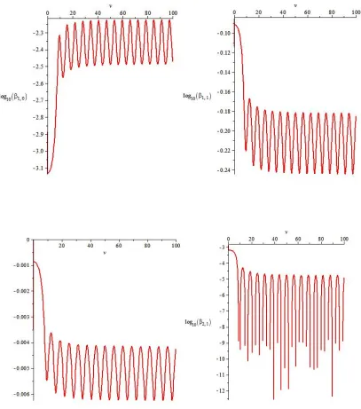
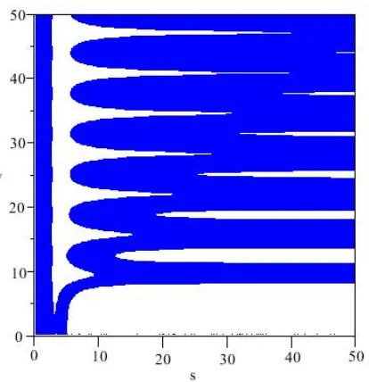
h,is the frequency and his the step length. The behavior of the coefficients of the PL method are shown in Figure 1. In Figure 2, we present the sv plane (stabilityFigure 2.s−v plane of the new obtained method PL′′′.
2.2. THE SECOND FORMULA
If P1, K 5, so we called PL,we have
, ) 12 cos 12 cos 5 ( cos 120 120 56 cos 4 3 120 1 , 10 20 1 , 12 30 1 , 24 15 14 2 2 2 2 2 4 1 , 2 1 , 2 0 , 2 1 , 2 1 , 1 1 , 2 0 , 1 v v v v v v v v v v
For small values of vthe above formulae are subject to heavy cancelations. In this case the following Taylor series expansion must be used:
, 792000
6564076705 1229606918
60887 7456104624 0
0950838272 2054481067
39 2223525220
98432000 1089933508
2072169709 7280
3460106377 11233841 0
2640496320 139199 762048
59 15120
13
12 10
8 6
4 2
0 , 2
v v
v v
v v
, 96000
2820383528 6148034593
12943 5494232445 0
5475419136 1027240533
31 1707252643
9216000 5449667544
1694889341 728
3460106377 2074145 0
1320248160 205351 381024
295 7560
313
12 10
8 6
4 2
1 , 2
v v
v v
v v
The phase-lag and the local truncation error for the PL,method are given by
, 8745608719468071
3328231 14 16
v O v
plPL
and
'''
4 (6 ) (10) 2 (8) 10
59
4 ( ) ( ) 5 ( ) ,
76204800
PL
LTE D y x D y x D y x h
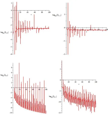
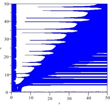
where h, ,is the frequency and h,is the step length. The behavior of the coefficients of the PL'', method are shown in Fig. 3. In Fig. 4 we present the svplane (stability region) for the method PL''.
The characteristic equation
s:v2
A(v)s2 2B(v)sA(v)0has complex rootsof unit magnitude when
1,) (
) ( ) (
cos
v A
v B
v or A(v)2 B(v)2 0.
Substituting A(v)andB(v)for these the two-step methods, the interval of periodicity of the
Figure 4.s−v plane of the the new obtained method PL′′.
3.
N
UMERICALE
XAMPLESIn this section, we present some numerical results obtained by our new two-step trigonometrically-fitted Obrechkoff methods and compare them with those from other multistep methods as
Simos: The 12th order Obrechkoff method of Simos [24].
Daele: The 12th order Obrechkoff method of Van Daele [26].
Achar: The 8th order Obrechkoff method of Achar [1].
Wang: The 12th order Obrechkoff method of Wang [30].
Example 3.1. We consider the nonlinear undamped Duffingequation
0 0, (12) ', 67 2004267280 .
0 ) 0 ( ), cos( 3
''yy B x y y
y
Where B0.002, 1.01and .
01 . 1
5 . 40 ,
0
x We use the following exact solution for
(12),g(x)
i30K2i1cos
(2i1)x
,where. } 10 374 . 0 , 10 304016 .
0
, 10 246946143 .
0 , 36 2001794775 .
0 { } , , , {
9 6
3 7
5 3 1
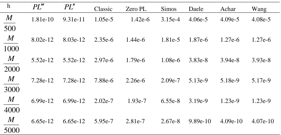
Table 1: Comparison of the end-point absolute error in the approximations obtained by using Methods: the classical method, methods of Simos, Daele, Achar, Wang, zero phase-lag and the new methods for Example 3.1.
h PL PL
Classic Zero PL Simos Daele Achar Wang
500
M 1.81e-10 9.31e-11 1.05e-5 1.42e-6 3.15e-4 4.06e-5 4.09e-5 4.08e-5
1000
M 8.02e-12 8.03e-12 2.35e-6 1.44e-6 1.81e-5 1.87e-6 1.27e-6 1.27e-6
2000
M 5.52e-12 5.52e-12 2.97e-6 1.79e-6 1.08e-6 3.83e-8 3.94e-8 3.93e-8
3000
M 7.28e-12 7.28e-12 7.88e-6 2.26e-6 2.09e-7 5.13e-9 5.18e-9 5.17e-9
4000
M 6.99e-12 6.99e-12 2.02e-7 1.93e-7 6.55e-8 3.19e-9 1.23e-9 1.23e-9
5000
M 6.65e-12 6.65e-12 5.95e-7 2.81e-7 2.67e-8 9.89e-10 4.09e-10 4.07e-10
In order to integrate this equation by a Obrechkoff method, one needs the values of y′,
which occur in calculating (4).
y These higher order derivatives can all be expressed in terms
of y(x) and y′(x) through (12), i.e.
1 3 ( )
( ) sin( ), )( 2
) 3 (
x B
x y x y x
y
1 3 ( )
( ) 6 ( ) ( ) cos( ), )( 2 2 2
) 4 (
x B
x y x y x y x y x
y
The absolute errors at x40.5/(1.01),for the new method, in comparison with methods of
classical method, zero phase-lag method, Simos, Daele, Achar, Wang and the new methods are given in table 1 and the CPU times are listed in Table 2.
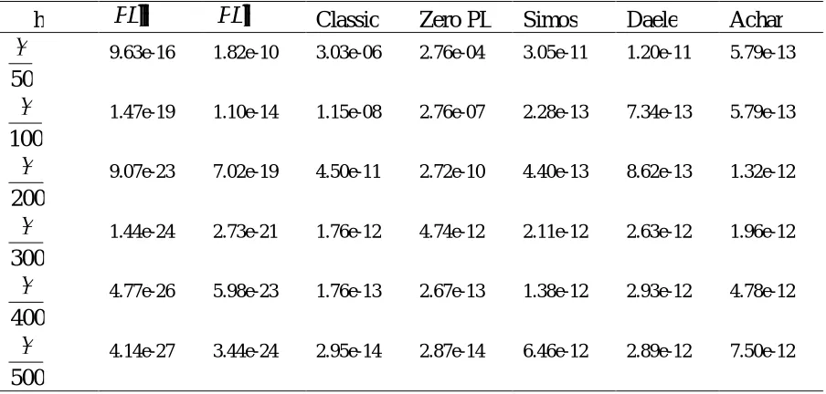
Example 3.2. Consider the initial value problem y100y99sin(x),
, 11 ) 0 ( ' , 1 ) 0
( y
y with the exact solution y(t)sin(t)sin
10t
cos
10t
.This equation has been solved numerical for 0x10 using exact starting values. In the numerical experiment, we take the step lengths h/50,/100,/200,/300,/400 and /500.In Table 3, we present the absolute errors at the end-point and the CPU times are listed in Table 4.
0,4.5
, ,2 ) 0 ( , 1 ) 0 ( , 2 1
2 8
y y x
x y y
Table 2: CPU time for the example 3.1, are calculated for comparison among eight methods: the classical method, methods of Simos, Daele, Achar, Wang, zero phase-lag and the new methods.
h PL PL
Classic Zero PL Simos Daele Achar Wang
500
M 1.1 1.1 1.1 1 1.4 1.5 1.2 1.4
1000
M 2.2 2.1 2.2 2.2 2.9 2.9 2.3 2.9
2000
M 4.3 4.6 4.4 4.4 6.2 6.3 4.8 6.2
3000
M 7.2 7.8 7.5 7.5 9.8 9.7 7.5 9.5
4000
M 10 10.6 9.8 10 13.5 13.3 10 13
5000
M 12 13.3 14 13 17 17 12.9 16.5
Table 3: Comparison of the end-point absolute error in the approximations obtained by using Methods: the classical method, methods of Simos, Daele, Achar, zero phase-lag and the new methods for Example 3.2.
h PL PL Classic Zero PL Simos Daele Achar
50
9.63e-16 1.82e-10 3.03e-06 2.76e-04 3.05e-11 1.20e-11 5.79e-13
100
1.47e-19 1.10e-14 1.15e-08 2.76e-07 2.28e-13 7.34e-13 5.79e-13
200
9.07e-23 7.02e-19 4.50e-11 2.72e-10 4.40e-13 8.62e-13 1.32e-12
300
1.44e-24 2.73e-21 1.76e-12 4.74e-12 2.11e-12 2.63e-12 1.96e-12
400
4.77e-26 5.98e-23 1.76e-13 2.67e-13 1.38e-12 2.93e-12 4.78e-12
500
Table 4: CPU time for the example 3.2, are calculated for comparison among seven methods: the classical method, methods of Simos, Daele, Achar, zero phase-lag and the new methods.
h PL PL Classic Zero PL Simos Daele Achar
50
0.14 0.23 0.12 0.11 0.17 0.25 0.19
100
0.44 0.37 0.33 0.45 0.51 0.53 0.45
200
0.89 0.87 0.9 0.89 0.86 0.83 0.75
300
1.35 1.3 1.4 1.3 1.14 1.15 0.95
400
1.8 1.8 1.9 1.8 1.39 1.40 1.23
500
2.3 2.3 2.3 2.3 1.70 1.78 1.47
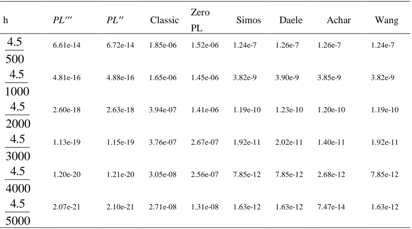
Table 5: Comparison of the end-point absolute error in the approximations obtained by using Methods: the classical method, methods of Simos, Daele, Achar, Wang, zero phase-lag and the new methods for Example 3.3.
h PL PL Classic Zero
PL Simos Daele Achar Wang
500 5 .
4 6.61e-14 6.72e-14 1.85e-06 1.52e-06 1.24e-7 1.26e-7 1.26e-7 1.24e-7
1000 5 .
4 4.81e-16 4.88e-16 1.65e-06 1.45e-06 3.82e-9 3.90e-9 3.85e-9 3.82e-9
2000 5 .
4 2.60e-18 2.63e-18 3.94e-07 1.41e-06 1.19e-10 1.23e-10 1.20e-10 1.19e-10
3000 5 .
4 1.13e-19 1.15e-19 3.76e-07 2.67e-07 1.92e-11 2.02e-11 1.40e-11 1.92e-11
4000 5 .
4 1.20e-20 1.21e-20 3.05e-08 2.56e-07 7.85e-12 7.85e-12 2.68e-12 7.85e-12
5000 5 .
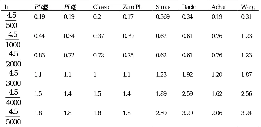
Table 6: CPU time for the example 3.3, are calculated for comparison among eight methods: the classical method, methods of Simos, Daele, Achar, Wang, zero phase-lag and the new methods.
h PL PL Classic Zero PL Simos Daele Achar Wang
500 5 .
4 0.19 0.19 0.2 0.17 0.369 0.34 0.19 0.31
1000 5 .
4 0.44 0.34 0.37 0.39 0.62 0.61 0.76 1.23
2000 5 .
4 0.83 0.72 0.72 0.75 0.62 0.61 0.76 1.23
3000 5 .
4 1.1 1.1 1 1.1 1.23 1.92 1.20 1.87
4000 5 .
4 1.5 1.4 1.5 1.4 1.89 2.59 1.62 2.56
5000 5 .
4 1.8 1.8 1.8 1.8 2.59 3.29 2.06 3.24
with the exact solution
. 2 1
1 ) (
x x
y
The absolute errors atx4.5for the new methods, in comparison with methods of Wang, Simos, Daele, Achar, classical method and zero phase-lag method are given in Table 5. The relative CPU times of computation of the new methods in comparison with the other six our referred methods are given in Table 6.
4.
C
ONCLUSIONSIn this paper, we have presented the new trigonometrically-fitted two-step symmetric Obrechkoff method of order8. The details of the procedure adapted for the applications have been given in Section 2. With trigonometric fitting, we have improved the local truncation error, phase-lag error, interval of periodicity and CPU time for the classes of two-step Obrechkoff methods. The numerical results obtained by the new method for some problems show its superiority in efficiency, accuracy and stability.
R
EFERENCES1. Achar, S. D., Symmetric multistep Obrechkoff methods with zero phase-lag for periodic initial value problems of second order differential equations, J. Appl. Math. Comput. 218 (2011) 22372248.
2. Alolyan, I., Simos, T. E., Mulitstep methods with vanished phase-lag and its firstand second derivatives for the numerical integration of the Schrödinger equation, J. Math. Chem. 48 (4) (2010) 10921143.
3. Ananthakrishnaiah, U. A., P-stable Obrechkoff methods with minimal phase-lag for
periodic initial value problems, Math. Comput. 49 (1987) 553559.
4. Chawla, M. M., Rao, P. S., A Numerov-type method with minimal phase-lag for the
integration of second order periodic initial value problems. ii: Explicit method, J. Comput. Appl. Math. 15 (1986) 329337.
5. Dahlquist, G., On accuracy and unconditional stability of linear multistep methods for second order differential equations, BIT 18 (2) (1978) 133136.
6. Franco, J. M., An explicit hybrid method of Numerov type for second-order periodic initial-value problems, J. Comput. Appl. Math. 59 (1995) 7990.
7. Franco, J. M., Palacios, M., High-order P-stable multistep methods, J. Comput Appl. Math. 30 (1) (1990) 110.
8. Gautschi, W., Numerical integration of ordinary differential equations based on trigonometric polynomials, Numer. Math. 3 (1961) 381397.
9. Hairer, I. E., Unconditionally stable methods for second order differential equations, Numer. Math. 32 (1979) 373379.
10.Henrici, P., Discrete variable methods in ordinary differential equations. Wiley, New York (1962).
11.Ixaru, L. Gr., Rizea, M., A Numerov-like scheme for the numerical solution of the Schrödinger equation in the deep continuum spectrum of energies, Comput. Phys. Commun. 19 (1) (1980) 2327.
12.Jain, M. K., Jain, R. K. and Krishnaiah, U. A., Obrechkoff methods for periodic initial value problems of second order differential equations, J. Math. Phys. 15
(1981) 239250.
13.Lambert, J. D., Numerical methods for ordinary differential systems, The Initial Value Problem, John Wiley and Sons, (1991).
14.Lambert, J. D., Watson, I. A., Symmetric multistep methods for periodic initial value problems, J. Inst. Math. Appl. 18 (1976) 189202.
15.Neta, B., P-stable symmetric super-implicit methods for periodic initial value problems, Comput. Math. Appl. 50 (2005) 701705.
16.Quinlan, G. D., Tremaine, S., Symmetric multistep methods for the numerical integration of planetary orbits, The Astro. J. 100 (5) (1990) 16941700.
17.Ramos, H., Vigo-Aguiar, J., On the frequency choice in trigonometrically fitted methods, Appl. Math. Lett. 23 (11) (2010) 13781381.
19.Raptis, A. D., Exponentially-fitted solutions of the eigenvalue Shrödinger equation with automatic error control, Comput. Phys. Commun. 28 (1983) 427431.
20.Saldanha, G., Achar, S. D., Symmetric multistep Obrechkoff methods with zero phase-lag for periodic initial value problems of second order differential equations, J. Appl. Math. Comput. 218 (2011) 22372248.
21.Shokri, A., The symmetric two-step P-stable nonlinear predictor-corrector methods for the numerical solution of second order initial value problems, Bull. Iran. Math. Soc., in press.
22.Shokri, A., Saadat, H., Trigonometrically fitted high-order predictorcorrector method with phase-lag of order infinity for the numerical solution of radial Schrödinger equation, J. Math. Chem. 52 (7) (2014) 18701894.
23.Shokri, A., Saadat, H., High phase-lag order trigonometrically fitted two-step Obrechkoff methods for the numerical solution of periodic initial value problems, Numer. Algor. DOI: 10.1007/s11075-014-9847-7.
24.Simos, T. E., A P-stable complete in phase Obrechkoff trigonometric fitted method for periodic initial value problems, Proc. R. Soc. 441 (1993) 283289.
25.Steifel, E., Bettis, D. G., Stabilization of Cowells methods, Numer. Math. 13 (1969) 154175.
26.Van Daele, M., Vanden Berghe, G., P-stable exponentially fitted Obrechkoff methods of arbitrary order for second order differential equations, Numer. Algor. 46
(2007) 333350.
27.Vanden Berghe, G., Van Daele, M., Trigonometric polynomial or exponential fitting approach, J. Comput. Appl. Math. 233 (2009) 969979.
28.Wang, Z., Wang, Y., A new kind of high efficient and high accurate P-stable Obrechkoff three-step method for periodic initial value problems, Comput. Phys. Commun. 171 (2) (2005) 7992.
29.Wang, Z., Zhao, D., Dai, Y. and Song, X., A new high efficient and high accurate
Obrechkoff four-step method for the periodic non-linear undamped duffings equation, Comput. Phys. Commun. 165 (2005) 110126.
30.Wang, Z., Zhao, D., Dai, Y. and Wu, D., An improved trigonometrically fitted P-stable Obrechkoff method for periodic initial value problems, Proc. R. Soc. 461