Evaluation of 4 years of continuous 13 C(CO 2) data using a moving Keeling plot method

www.biogeosciences.net/13/4237/2016/ doi:10.5194/bg-13-4237-2016

© Author(s) 2016. CC Attribution 3.0 License.

Evaluation of 4 years of continuous

δ

13

C(CO

2

) data using a moving

Keeling plot method

Sanam Noreen Vardag, Samuel Hammer, and Ingeborg Levin

Department of Physics and Astronomy, Institut für Umweltphysik, Heidelberg University, Heidelberg, Germany Correspondence to:Sanam Noreen Vardag ([email protected])

Received: 15 March 2016 – Published in Biogeosciences Discuss.: 16 March 2016 Revised: 8 July 2016 – Accepted: 8 July 2016 – Published: 26 July 2016

Abstract. Different carbon dioxide (CO2) emitters can be distinguished by their carbon isotope ratios. Therefore mea-surements of atmosphericδ13C(CO2) and CO2concentration contain information on the CO2 source mix in the catch-ment area of an atmospheric measurecatch-ment site. This infor-mation may be illustratively presented as the mean isotopic source signature. Recently an increasing number of contin-uous measurements of δ13C(CO2) and CO2 have become available, opening the door to the quantification of CO2 shares from different sources at high temporal resolution. Here, we present a method to compute the CO2source sig-nature (δS) continuously and evaluate our result using model data from the Stochastic Time-Inverted Lagrangian Transport model. Only when we restrict the analysis to situations which fulfill the basic assumptions of the Keeling plot method does our approach provide correct results with minimal biases in

δS. On average, this bias is 0.2 ‰ with an interquartile range of about 1.2 ‰ for hourly model data. As a consequence of applying the required strict filter criteria, 85 % of the data points – mainly daytime values – need to be discarded. Ap-plying the method to a 4-year dataset of CO2andδ13C(CO2) measured in Heidelberg, Germany, yields a distinct seasonal cycle ofδS. Disentangling this seasonal source signature into shares of source components is, however, only possible if the isotopic end members of these sources – i.e., the biosphere,

δbio, and the fuel mix,δF– are known. From the mean source signature record in 2012, δbio could be reliably estimated only for summer to (−25.0±1.0) ‰ andδF only for win-ter to (−32.5±2.5) ‰. As the isotopic end membersδbio andδFwere shown to change over the season, no year-round estimation of the fossil fuel or biosphere share is possible from the measured mean source signature record without

ad-ditional information from emission inventories or other tracer measurements.

1 Introduction

A profound understanding of the carbon cycle requires clos-ing the atmospheric CO2 budget at a regional and global scale. For this purpose it is necessary to distinguish be-tween CO2 contributions from oceanic, biospheric and an-thropogenic sources and sinks. Monitoring these CO2 con-tributions separately is desirable to improve process under-standing, to investigate climatic feedbacks on the carbon cy-cle and also to verify emission reductions and design CO2 mitigation strategies (Marland et al., 2003; Gurney et al., 2009; Ballantyne et al., 2010).

A possibility to distinguish between different CO2sources and sinks utilizes concurrent12CO2and13CO2observations in the atmosphere. The carbon isotope ratio can be used to identify and even quantify different CO2 emitters if every emitter has its specific knownδ13CO2signature. For exam-ple, the CO2fluxes from land and ocean can be distinguished using the ratio of stable carbon isotopologue13CO2/12CO2in addition to CO2concentration measurements (Mook et al., 1983; Ciais et al., 1995; Alden et al., 2010). In other studies, measurements of13CO2 have been used to distinguish be-tween different fuel types (Pataki, 2003; Lopez et al. 2013; Newman et al., 2016) or to evaluate ecosystem behavior (Torn et al., 2011), to mention but a few examples of the many published in the literature.

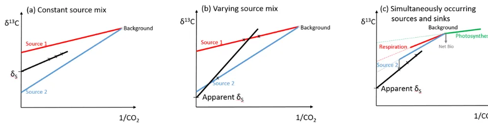
measure-Figure 1.Regression-based determination of source signature using a Keeling plot. For clarity of illustration, we only draw three data points instead of five, which we use for our computation.(a)Constant source mix during the time of source signature determination leads to the correct flux-weighted mean isotopic signature (following Eq. A1),δS.(b)Change of source mix during the period of determination of a Keeling plot due to either a temporal change of emission characteristics or a wind direction change (transportation) leads to a biased result. These situations can be usually identified by a large error of the intercept,δS(we choose an error>2 ‰ to reject these results).(c)Sources and sinks with different isotopic signatures or sink fractionation occur at the same time and lead to a wrong apparent source signature. Strong biases are prevented by choosing a minimum net CO2concentration range of 5 ppm and demanding a monotonous increase of CO2during the 5 h (see text for more details). Note that the background value is displayed for illustration, but it is not used in the moving Keeling plot method.

ments. This has led to an increasing deployment of these in-struments, thereby increasing the temporal and spatial res-olution of 13C(CO2) and CO2 data (Bowling et al., 2003; Tuzson et al., 2008; McManus et al., 2010; Griffith et al., 2012; Vogel et al., 2013; Vardag et al., 2015a; Eyer et al., 2016). These data records may lead to an improved under-standing of regional CO2fluxes, allowing estimates of mean

δ13C source signatures at high temporal resolution. Estimat-ing mean source signatures from concurrentδ13C(CO2) and CO2 records over time provides, e.g., insight into temporal changes in the signatures of two different CO2sources such as fossil fuels and the biosphere if their relative share to the CO2offset is known. This may be used to study biospheric responses to climatic variations like drought, heat, floods, va-por pressure deficit etc. (Ballantyne et al., 2010; 2011; Bas-tos et al., 2016). Likewise, the mean source signature can be used to separate between different source CO2contributions if the isotopic end members of these sources are known at all times (Pataki, 2003; Torn et al., 2011; Lopez et al. 2013; Moore and Jacobson, 2015; Newman et al., 2016).

Many studies have successfully used the Keeling or Miller–Tans plot method (Keeling, 1958; 1961; Miller and Tans, 2003) to determine source signatures in specific set-tings (e.g., Pataki, 2003; Ogée et al., 2004; Lai et al., 2004; Knohl et al., 2005; Karlsson et al., 2007; Ballantyne et al., 2010). However, the situations in which Keeling and Miller– Tans plots yield correct results need to be selected carefully (Miller and Tans, 2003). Only if all possible pitfalls are pre-cluded can the Keeling intercept (or the Miller–Tans slope) be interpreted as the gross flux-weighted mean isotopic sig-nature of all CO2 sources and sinks in the catchment area of the measurement site. Especially in polluted areas with variable source–sink distribution, estimation of isotopic

sig-nature using a Keeling or Miller–Tans plot requires a solid procedure, e.g., accounting for wind direction changes or si-multaneously occurring CO2sinks and sources.

In this study, we discuss the possible pitfalls of CO2source signature determination from a continuous dataset using the Keeling plot method and follow a specific modification of this method for automatic retrieval of mean source signa-ture with minimal biases. We test this method with model-simulated CO2mole fraction and δ13C(CO2) data. Using a modeled dataset where all source signatures are known en-ables us to test if the calculated source signature is correct, which is vital when evaluating measured data with an auto-mated routine. Having found a method to determine the iso-topic signature of the mean source correctly from measured CO2andδ13C(CO2) data, we discuss which information can be reliably extracted from these results.

2 Methods

2.1 Keeling and Miller–Tans plot method

Keeling (1958, 1961) showed that the mean isotopic signa-ture of a source mix can be calculated by re-arranging the mass balance of total CO2,

CO2tot=CO2bg+CO2S, (1)

and ofδ13C of total CO2, i.e.,δtot,

δtot·CO2tot=δbg·CO2bg+δS·CO2S (2) to

where CO2bgandδbgare the concentration andδ13C(CO2) of the background component and CO2SandδSare the concen-tration andδ13C(CO2) of the mean source, respectively. Plot-tingδtotvs. 1 / CO2totyields ay intercept ofδS(cf. Fig. 1a).

Miller and Tans (2003) have suggested an alternative approach to determine the mean isotopic signature by re-arranging Eqs. (1) and (2) such thatδSis the regression slope when plotting CO2tot·δtotvs. CO2tot:

CO2tot·δtot=δS·CO2tot−CO2bg(δbg−δS). (4) They argue that this approach might be advantageous since the isotopic signature does not need to be determined from extrapolation to 1/CO2=0, which could introduce large errors in the δS estimate. Zobitz et al. (2006) have com-pared the Keeling and the Miller–Tans plot method (Eqs. 3 and 4) and found no significant differences between both approaches when applied to typical ambient CO2 varia-tions. We were able to reproduce this result with our model-simulated dataset (cf. Sect. 3.1). Differences between both approaches were (0.00±0.04) ‰ when applying certain criteria (standard deviation of intercept <2 ‰, CO2 range within 5 h>5 ppm), which will be explained in Sect. 2.3. The choice of fitting algorithm has also been discussed in the literature. Pataki (2003), Miller and Tans (2003) and Zo-bitz et al. (2006) compared different fitting algorithms for the regression and came up with different recommendations. Or-thogonal distance regression (ODR) and weighted total least-squares (WTLS) fits (model 2 fits) take into account errors onxandy, whereas ordinary least-squares (OLS) minimiza-tion (model 1 fit) only takes into account y errors. Zobitz et al. (2006) have found differences between both fitting al-gorithms especially at small CO2 ranges. We have also ap-plied a model 1 (OLS) and model 2 (WTLS) fit to our sim-ulated data and have not found any significant differences ((0.00±0.01) ‰) between them when applying certain crite-ria (error of intercept<2 ‰, CO2range within 5 h>5 ppm; see Sect. 2.3). In our study, we use a WTLS fit (Krystek and Anton, 2007) as a stable algorithm for fitting a straight line to a dataset with uncertainty inxandy direction in a Keel-ing plot method. Note that the isotopic signature of the mean sourceδScan be determined from linear regression without requiring a background CO2andδ13C(CO2) value. However, the Keeling and Miller–Tans plot methods are only valid if the background and the isotopic signature of the source mixδS are constant during the period investigated (Keeling, 1958; Miller and Tans, 2003). Further, the approaches are only valid when sources and sinks do not occur simultane-ously. Miller and Tans (2003) gave an example which showed that as soon as sources and sinks of different isotopic signa-ture/fractionation occur simultaneously, the determination of isotopic signature of the source–sink mix may introduce bi-ases. In these cases, the results cannot be interpreted as mean flux-weighted source signature anymore. This has very un-fortunate consequences, since in principle we are interested in determining the isotopic signature of the source mix of a

region during all times, i.e., also during the day, when photo-synthesis cannot be neglected.

2.2 Moving Keeling plot method

For a continuous long-term dataset, we suggest an auto-matic routine to determine the mean isotopic signature of the source mix. It is similar to the moving Keeling plot for CH4 currently suggested by Röckmann et al. (2016). In our case of CO2, we also have to take into account the possibility of simultaneously occurring sinks and sources, which is not im-portant in the case of CH4. Our moving Keeling plot method is a specific case of the classical Keeling plot method (Eq. 3) (Keeling, 1961) as it uses only five hourly-averaged measure-ment points of CO2andδ13C(CO2), fitting a regression line through these five data points (cf. Fig. 1a, illustrated only for three data points for clarity of inspection). We choose 5 h as a compromise between number of data points, and thus of robust regression, and of source mix constancy. This com-promise also manifests itself in such a manner that a win-dow size of 5 h leads to maximum coverage. No background value is included in the regression. The moving Keeling plot method works such that, e.g., for the determination of the mean source signature at 15:00, we use the hourly CO2and

δ13C(CO2) measurements from 13:00 to 17:00 and fit a re-gression line. Next, for the determination of the source signa-ture at 16:00, we use the CO2andδ13C(CO2) measurements from 14:00 to 18:00 and so on. Note that this approach leads to a strong autocorrelation of neighboring source signature values.

2.3 Filter criteria of the moving Keeling plot method

In order to prevent pitfalls in the regression-based determi-nation of mean isotopic signature, we set a few criteria for the moving Keeling plots to “filter” out situations in which a Keeling plot cannot be performed. These filter criteria are also similar in type to the ones introduced by Röckmann et al. (2016). We here explain why these filter criteria are needed for CO2and how they are set.

de-crease would be due to either a sink of CO2or a breakdown of the boundary layer inversion potentially associated with a change of catchment area of the measurement, both biasing the resulting mean source signature.

As mentioned before, the determination of a mean isotopic signature is not per se possible during the day when CO2 sinks and sources are likely to occur simultaneously (Miller and Tans, 2003). This can be explained in the Keeling plot by the vector addition of CO2source and sink mixing lines with different isotopic signatures, resulting in a vector with an intercept different from the expected one, leading to an isotopic signature which can even lie outside the expected range of the isotopic source end members (see Fig. 1c). This potential bias is stronger the smaller the net CO2signal is. Therefore, e.g., for evaluation of the Heidelberg data, we de-mand an increase in CO2 during the 5 h period of at least 5 ppm to exclude periods where the photosynthetic sink is similarly strong to total CO2sources. This normally leads to an exclusion of daytime periods, when the boundary layer inversion typically breaks up and the photosynthetic sink is most pronounced. Therefore, we are mainly rejecting periods in which isotopic discrimination during photosynthesis dom-inates the mean isotopic source signature. During winter, it may happen that the inversion does not break up due to the cold surface temperatures, but in this season photosynthetic activity is typically much smaller than fossil fuel emissions, and therefore biases of the regression-based mean source sig-nature are only small.

In the next section, we show that with these filter cri-teria – i.e., (i) error of the Keeling plot intercept <2 ‰, (ii) monotonous increase during 5 h and (iii) increase of

>5 ppm during 5 h, which we chose empirically – we are able to successfully reject those source signatures where the underlying assumptions for the Keeling plot method are not met. In Sect. 3.1, we will also briefly discuss how sensitive the result is to the choice of filter criteria. Note that the filter criteria may differ for different measurement sites depending on the source heterogeneity and footprint of the catchment areas. Therefore, respective filter criteria need to be designed individually for each measurement station.

3 Results and discussion

3.1 Evaluation of the moving Keeling plot method

We apply the moving Keeling plot method to a modeled CO2 and δ13C(CO2) dataset. As also pointed out by Röckmann et al. (2016) in their CH4study, this has the advantage that we can test and evaluate our filter criteria as we know ex-actly the individual isotopic source signatures that created the modeled dataset and, thus, the contribution-weighted mean isotopic source signature at every point in time. Details on the Stochastic Time-Inverted Lagrangian Transport (STILT) model (Lin et al., 2003) and on the computation of the

mod-eled CO2 andδ13C(CO2) record as well as of the resulting mean source signature,δ_SSTILT, are given in Appendix A.

We apply the same filter criteria to the calculated mean source signature of the STILT-modeled datasetδ_SSTILTas to the regression-based mean source signature (Sect. 2.3). The “unfiltered” source signatures (black in Fig. 2a) are 0–2 ‰ more enriched than the “filtered” source signatures (blue). This offset is mainly caused by the daytime source signa-tures, which are on average more enriched than nighttime source signatures (Fig. 2b) but more likely to be filtered out based on the criteria of Sect. 2.3.

We have now evaluated the moving Keeling plot method and the used filter criteria based on the model data and tested whether they allow a bias-free retrieval of the mean source signature. In Fig. 3a, we compare the regression-based source signatures to the filtered reference source sig-nature of Fig. 2a, which we have extracted from the model. We compare not only the mean difference of the mean source signature but also the hourly differences of the mean source signature as well as the smoothed difference. This enables us to clearly state how well we are able to determine the hourly mean source signature and its long-term trend.

Figure 3a displays the filtered seasonal changes of the source signature exemplary for the year 2012. The moving Keeling plot method is able to extract the seasonal vari-ability of the mean isotopic signature correctly. The median difference (and interquartile range) between the smoothed regression-based (red) and smoothed modeled (blue) ap-proach (both smoothed with 50th-percentile filter with win-dow size of 100 h, no smoothing 50 points in front of large data gaps) is 0.0±0.4 ‰. A smoothing window size of 100 h (ca. 4 days) was chosen, so that synoptical and seasonal vari-ations of δS can be seen while diurnal variations are sup-pressed. On a shorter diurnal timescale, we compare individ-ual hourly results for the source signature (stars in Fig. 3b, c). The interquartile range of the filtered hourly difference between the referenceδ_SSTILT and the moving Keeling plot signature is about 1.2 ‰ throughout the year, but the me-dian difference is small (0.2 ‰). The source signature of the model reference and moving Keeling plot source signature show the same temporal pattern both in summer and in win-ter. Further, we find that, if we do not apply all of the criteria described in Sect. 2.3 (unfiltered data in Fig. 3b, c), we see larger differences between regression-based source signature (from the moving Keeling plot) and the STILT reference val-ues.

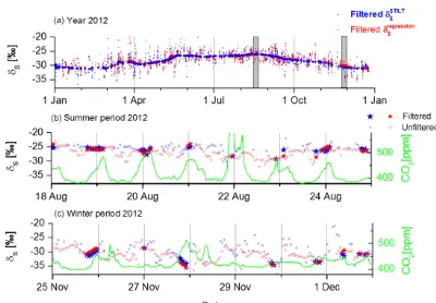
Figure 2.Source signature as calculated with the STILT model following Eq. (A1).(a)Unfiltered in black and filtered (for monotonous increase and minimal range) in blue. Only about 15 % of all data points fulfill our strict criteria. However, they are distributed approximately evenly throughout the year.(b)Diurnal cycle of modeled mean source signature due to diurnally varying mean source mix. Gray areas denote times when source signature is usually filtered out.

no criteria for the minimal CO2range, but only for the error of the intercept (<2 ‰), about 60 % of all data remain for the estimated source signature, but the median difference be-tween model- and Keeling-based results increases to 0.3 ‰, and the interquartile range increases to 2.4 ‰ (hourly data), which is about twice what we found before. Withdrawing all filter criteria and using only nighttime values leads to a cov-erage of about 35 % (nighttime) and an interquartile range of 3.5 ‰. The filter criteria which we use here (Sect. 2.3) are, thus, rather strict, but we are confident to precisely extract the correct source signature from theδ13C(CO2) and CO2record at the highest temporal resolution.

3.2 The measured source signature record in Heidelberg

We now apply this approach to real measured Heidelberg data. We use the CO2andδ13C(CO2) record at hourly time resolution (Fig. B1) to compute the isotopic source signa-ture via regression (Fig. 4). The quality of the CO2 and

δ13C(CO2) record is assessed in Appendix B. The measure-ment site and its surrounding catchmeasure-ment area are described by Vogel et al. (2010). We observe a distinct seasonal cycle of the mean isotopic source signature in Heidelberg. Smoothed minimum values of about−32 ‰ are reached in winter. Max-imum values of about−26 ‰ occur in summer. This annual pattern is reproduced every year and is similar to annual pat-terns observed by, e.g., Schmidt (1999) for Schauinsland, Germany, or by Sturm et al. (2006) for Bern, Switzerland. Additionally, the first year shows a more enriched summer maximum source signature. A number of data points (fewer than 0.5 %) lie outside the range of realistic end members be-tween−20 and−45 ‰ of any source in the catchment area (see Table A1). These outliers are not unusual in an urban setting, as the interquartile range of the modeled δS for the Heidelberg catchment area is about 1.2 ‰ for hourly (non-smoothed) data, which is only about 30 % higher than the interquartile range of the measured data (see Fig. 4 (1.8 ‰)). The slightly lower variability in the model may be due to a lower variability in the coarse-resolution emission inventory used in STILT (0.1◦×0.1◦).

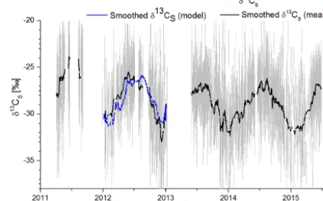
Our 4-year record of the mean source signature in Hei-delberg (see Fig. 4) provides a first insight into the source characteristics at the measurement station. It reaches its min-imum in winter, when we expect residential heating (mainly isotopically depleted natural gas; see Table A1) to contribute significantly to the source mix. The source signature reaches its maximum in summer, when more enriched biospheric fluxes are expected to dominate the CO2 signal. This ob-served seasonal cycle in Heidelberg is very similar to the filtered modeled source signature in amplitude as well as in phase (blue line in Fig. 4).

Figure 4. Moving Keeling plot method-based source signature in Heidelberg from 2011 until mid-2015. The black line is the smoothed measured source signature, and the blue line gives the smoothed modeled source signature (both 50th-percentile filter with window size=100 h). Half a window size before the beginning of a large data gap the data are not further smoothed to prevent smooth-ing artifacts.

3.3 Information content derived fromδS

We now want to elaborate what quantitative information can be drawn from the mean source signature record in Heidel-berg about its components. For an urban continental mea-surement site, we have to assume that there are at least two main source types of CO2in the catchment area: fuel CO2 and CO2from the biosphere. In this simplest case, we essen-tially have one equation forδS (Eq. 6) with three unknown variables (δbio,δFand the fuel (or biosphere) sharefF); only if two of these variables are known can the third variable be quantified from the measurements:

δS= CO2F

1CO2 ·δF+

1CO2−CO2F

1CO2

·δbio (5) =fF·δF+(1−fF)·δbio. (6) Which of the variables is the one to be estimated depends, of course, on the research question. If the fossil fuel share and end members are well known from inventories, one could be especially interested in determining the isotopic end member

δbioin order to study biospheric processes and their feedback to climatic parameters (Ciais et al., 2005; Ballantyne et al., 2010; Salmon et al., 2011). Contrarily, one may be interested in determining the relative share of fossil fuel CO2 in the catchment area (with knownδbioandδF) to monitor emission changes independently from emission inventories.

by calibration with114C(CO2)) to calculate the fossil fuel CO2contribution from the (continuously) measured CO2and

δ13C(CO2) signal. However, knowing the isotopic signatures

δbio and δF over the entire course of the year requires an extensive number of measurements at the relevant sources throughout the year and further assumptions of how to scale up these point measurements to a mean source signature of all relevant sources. Therefore, the question, which we ad-dress here, is whether it is possible to obtain information on these end members from our measured source signature record, despite the fact that we have three unknown variables and only one equation. In the following, we discuss this ques-tion exemplary for the year 2012, for which we have modeled data, inventory information and the mean measured isotope signature. We restrict the discussion to a single year as we focus on discussing which information can principally be ob-tained from a year-round mean source signature record.

We have noted that, in order to obtain information fromδS on δbio (δF), we require information on the fuel CO2share andδF (on the fuel CO2 share andδbio). However, in cases where the relative share of the biosphere (fossil fuels) is neg-ligible, the isotopic signature of δF (δbio) would equal the mean measured isotopic signature. In these cases, the num-ber of unknown variables would be reduced to one, as the fos-sil fuel (biospheric) share is≈100 % andδbio(δF) does not contribute to the mean source signature. In a typical catch-ment area, the relative share of fossil fuels and of the bio-sphere will not be negligible throughout the year; however in winter, fossil fuel CO2will dominate, while in summer the biospheric CO2 will dominate the CO2 offset compared to the background. For example, from the STILT model results for Heidelberg (Sect. 3.1 and Appendix A), we perceive that on cold winter days in Heidelberg the fossil fuel share can be about 90 to 95 % of the total CO2 offset. In summer, it reaches a minimum of about 20 %. We may, thus, be able to obtain information about the isotopic end members ofδFin winter (δbioin summer), when the mean source signature is dominated by the fossil fuel (biospheric) share.

3.4 Evaluation ofδSin Heidelberg

To calculate the isotopic end members ofδi from the

mea-sured source signature in Heidelberg (and with that to solve Eq. 6), we require the fossil fuel CO2 share, which we take here from STILT and the bottom-up emission inven-tory Emissions Database for Global Atmospheric Research (EDGARv4.3; EC-JCR/PBL, 2015). However, as we only re-quire the share and not the absolute concentration, we are largely independent from potentially large model transport errors. We thus assume an absolute uncertainty of 10 % of the fossil fuel share (and of the biospheric share).

To determineδFin addition to the fuel CO2share, we re-quire a value for δbio. Here we use a typical mean value of the isotopic end member of δbio= −25.0 ‰ and assume a seasonal cycle as determined for Europe by Ballantyne et al.

(2011) (see Figs. 2 and 3 in Ballantyne et al., 2011) displayed in Fig. 5a as a solid green line. We showδbiowith two pos-sible uncertainties of 0.5 and 2.0 ‰. As expected, the un-certainty of the unknownδF is only acceptably small when the relative share of the biosphere becomes negligible, which is the case in winter (Fig. 5a). The isotopic end member of

δF in winter is about (−31.0±2.5) ‰ in January to March 2012 and decreases to (−32.5±2.5) ‰ in November to De-cember 2012. Further, Fig. 5a shows that the best estimate of the resulting isotopic signatureδFis more depleted in sum-mer than in winter. This curvature is the opposite of what we would expect from EDGAR transported by STILT (see assumedδFin Fig. 5b). Only when assuming an uncertainty of the biospheric end member of±2 ‰ or more, the uncer-tainty range of the estimatedδF allows a more enriched δF signature in summer than in winter. This suggests that the isotopic source signature of the biosphere in summer is most probably more depleted (by about 2 ‰) than the previously assumedδbiovalue based on Ballantyne et al. (2011).

To estimateδbio(Fig. 5b), we require (besides the fossil fuel share) the isotopic source signatureδF. Here we useδF calculated with the STILT model on the basis of EDGAR emissions and source signatures according to Table A1. Its annual mean value is−31.0 ‰, and it shows a seasonal cycle with more enriched signatures in summer than in winter. We show the results forδbiofor two possibleδFuncertainties of 1.0 and 3.0 ‰ (see Fig. 5b). The best estimate of the isotopic end member of δbio in summer is about −25.0±1.0 ‰ in June to August 2012. This reinforces the presumption that

δbiois more depleted than the assumedδbiovalue based on Ballantyne et al. (2011) during summer.

The uncertainty of the isotopic end members in Fig. 5a and b has three components: (1) the uncertainty of the fossil fuel CO2share estimated from STILT, which we assume to be about 10 % (absolute) in our case; (2) the uncertainty of the other known isotopic end member (0.5 and 2 ‰ forδbioor 1.0 and 3.0 ‰ forδF); and (3) the uncertainty of the measured mean source signature itself (ca. 0.4 ‰; see Sect. 3.1 for in-terquartile range of difference between smoothed regression-based and smoothed modeled source signature). Note that an uncertainty of 10 % of the fossil fuel share is at the low end of uncertainties. However, an uncertainty of 20 % of the fos-sil fuel share would increase the uncertainty in the unknown isotopic end members by only 0.2–0.4 ‰ forδbioin summer andδFin winter.

Figure 5. (a)A fixed isotopic end member of the biosphere (green,±uncertainty of 0.5 ‰ (light green area) and 2 ‰ (crosshatched green)) together with the measured source signature (black) results inδF(red,±its uncertainty).(b)A fixed isotopic end member of the fuel mix (red,

±uncertainty of 1.0 ‰ (salmon pink) and 2.0 ‰ (crosshatched gray-pink)) together with the measured source signature (black) results inδbio (green,±its uncertainty). In both cases, also the fuel CO2share (or biospheric CO2share) is required. We here use the share calculated with STILT on the basis of EDGAR v4.3 and assume an absolute uncertainty of 10 %.

June to August 2012, which is a very well constrained value for this period.

We cannot assume that the isotopic end membersδbioand

δFremain constant over the course of the year:δbiotypically shows a seasonal cycle possibly due to seasonal changes in the fraction of respiration from C3/C4 plants as well as due to influences of meteorological conditions on biospheric res-piration. Likewise, δF typically shows more enriched val-ues in summer, when the contribution of residential heating (and therewith of depleted natural gas) is much smaller than in winter. Therefore, no year-round estimation of fuel CO2 share is possible from only CO2andδ13C(CO2) either.

4 Summary and conclusions

Many measurement stations are currently being equipped with new optical instruments which measure δ13C(CO2), aiming at an improved quantitative understanding of the carbon fluxes in their catchment area. If this additional

δ13C(CO2) data stream is not directly digested in regional model calculations, the mean isotopic source signature is often computed from the δ13C(CO2) and CO2 records for a potential partitioning of source contributions. A bias-free determination of source signature, however, requires care-fully selecting the data for situations in which determina-tion of source signature with a Keeling plot method can

pro-vide reliable results. This excludes periods (1) when sinks and sources occur simultaneously, (2) when the source mix changes or (3) when the signal-to-noise ratio is too low (Keeling, 1958; 1961; Miller and Tans, 2003).

We therefore developed filter criteria and show that the routine and accurate determination ofδ13C(CO2) source sig-nature is possible if the introduced filter criteria are applied. As suggested by Röckmann et al. (2016), we use a modeled dataset for validation of the approach. We find that for a sta-tion like Heidelberg the bias introduced by our analysis is only (0.2±1.2) ‰ for hourly data. The uncertainty decreases in the long-term to (0.0±0.4) ‰. We are, therefore, able to estimate the source signature correctly, but 85 % of the data are rejected by the filter criteria. Further, as the filter crite-ria are such that the source signatures are more likely to be filtered out during the day than during the night, the long-term source signature is not representative of real daily av-erages, but only of periods where the data were not filtered out (mainly nighttime). As a consequence, the isotopic end membersδbioandδFcan also only be estimated for these pe-riods. This problem does not occur for CH4, which has only weak daytime sinks.

val-ues of about−26 ‰ in summer and about−32 ‰ in winter. This general behavior was expected due to the larger relative contribution of more depleted fossil fuel CO2in winter. For a unique interpretation of the mean source signature, possi-ble sources in the catchment area need to be identified. As soon as there is more than one source, the source signature is a function of the isotopic end members of all sources, as well as of their relative shares. Therefore, to study the sea-sonal and diurnal changes of fossil fuel shares at a continen-tal station, information on the isotopic end members of the fossil fuel mix as well as of the biosphere is required at the same time resolution. Unfortunately, the isotopic end mem-bers are often not known with high accuracy. The uncertainty of the isotopic end members often impedes or even prevents a unique straightforward determination of the source contri-bution in the catchment area (e.g., Pataki, 2003; Torn et al., 2011, Lopez et al. 2013; Röckmann et al., 2016) and calls for elaborated statistical models based on Bayesian statis-tics. This important fact is sometimes mentioned, but the consequences for quantitative evaluations are rarely empha-sized, preserving the high expectations associated with iso-tope measurements.

We showed that for the urban site of Heidelberg we can use the observation-based mean source signature record to estimate the isotopic end memberδF in winter and the iso-topic end memberδbioin summer within the uncertainties of ±2.5 and±1.0 ‰, respectively. Here we assumed an uncer-tainty of ±10 % for the fossil fuel and the biospheric CO2 share and an uncertainty of the other isotopic end memberδF of±3.0 ‰ andδbioof±2.0 ‰. However, in the winter sea-son we cannot obtain any reliable information on δbio, and in summer we cannot study δF. For a year-round determi-nation of fossil fuel share,δbioandδF are required through-out the year. As no reliable determination of δbio andδF is possible during the entire year based only on atmospheric observations, there is a need for either very good bottom-up information for the catchment area of interest or frequent measurement campaigns close to the sources. However, the disadvantage of using such a bottom-up approach is that usu-ally only information from a few specific sites are available, which need then to be upscaled correctly such that they are representative of the entire catchment area. For a determi-nation ofδF during the entire year, one can possibly utilize

114C(CO2) and CO/CO2 measurements (following Vardag et al. (2015b)) or O2/N2 measurements (e.g., Sturm et al. 2006; Steinbach et al., 2011), all of which exhibit their own deficiencies, which are discussed elsewhere (e.g., Ciais et al., 2015; Vardag et al., 2015b).

Finally, we could show that, even though it is not possible to determine the isotopic end members throughout the year, it is possible to refute certain literature values. For example, a respiration signature of−23 ‰ in August and September 2012 as reported by Ballantyne et al. (2011) is most likely too enriched as this would lead to more depletedδFvalues in summer than in winter. This is in contrast to what we would expect based on emission inventories.

5 Data availability

Appendix A: The STILT model

We use the STILT model (Lin et al., 2003) to evaluate our moving Keeling plot method. The STILT model computes the CO2 mole fraction by time-inverting meteorological fields and tracing particles emitted at the measurement loca-tion back in time to identify where the air parcel originated from. This so-called footprint area is then multiplied by the surface emissions in the footprint to obtain the CO2 concentration at the site in question. Photosynthesis and respiration CO2fluxes are taken from the vegetation photo-synthesis and respiration model (VPRM, Mahadevan et al., 2008). Anthropogenic emissions are taken from EDGAR v4.3 emission inventory (EC-JRC/PBL, 2015) for the base year 2010 and further extrapolated to the year 2012 using the BP Statistical Review of World Energy 2015 (available at http://www.bp.com/en/global/corporate/energy-economics/ statistical-review-of-world-energy/2015-in-review.html). Additionally, we use seasonal, weekly and daily time factors for different emission categories (Denier van der Gon et al., 2011). Since the EDGAR inventory is separated into different fuel types, we obtain a CO2 record for each fuel type as well as for respiration and photosynthesis. This allows us to construct a correspondingδ13C(CO2) record by multiplying the isotopic signature of every emission groupi

to its respective CO2 mole fractionδ13C(CO2)i·CO2,i (see

Table A1), adding these to a far-field boundary value of

δ13C(CO2)×CO2 and dividing it by the total CO2 at the model site. The CO2far-field boundary value for STILT is the concentration at the European domain border (16◦W to 36◦E and from 32 to 74◦N) at the position where the backwards-traced particles leave the domain. The concentra-tion at the domain border is taken from analyzed CO2fields generated with TM3 (Heimann and Körner, 2003) based on optimized fluxes (Rödenbeck, 2005). The isotopic boundary value is then constructed artificially by fitting the linear regression between CO2 and δ13C(CO2) in Mace Head (year 2011 from World Data Center for Greenhouse Gases; Dlugokencky et al. (2015)) and applying the function of the regression to the boundary CO2values in the model. Since, in reality, we also have measurement uncertainties of CO2 and δ13C(CO2), we also include a random measurement uncertainty of 0.05 ppm and 0.05 ‰, respectively, to the modeled datasets. The CO2andδ13C(CO2) records are used to calculate the regression-based mean source signature following the moving Keeling plot method (Sect. 2.2).

A1 Computation of mean modeled source signature

For the reference modeled mean source signature we use a “moving” background. In particular, we chose the mini-mum CO2value within 5 h centered around the measurement point as the background value and all contributions from fuel CO2(cF,i), respiration (cresp) and photosynthesis (cphoto) are computed as offsets relative to the background (cbg). This is then comparable to the regression-based moving Keeling plot method as the lowest and highest CO2values within 5 h span the Keeling plot. We are then able to define and compute the reference modeled mean source signature as

δ_SSTILT= P

iδF,i|cF,i| +δresp|cresp| +δphoto|cphoto|

P

i|cF,i| + |cresp| + |cphoto|

. (A1) Note that we use absolute values of all contributions since photosynthetic contributions (cphoto) are generally negative while source contributions (crespandcF,i) are generally

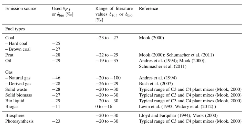
Table A1.δ13C(CO2) source signature of fuel types and biosphere as used in the model and the range of literature values. Note that for a specified region the range of possible isotopic signature can often be narrowed down if the origin and/or production process of the fuel type is known.

Emission source UsedδF,i

orδbio[‰]

Range of literature values δF,i or δbio [‰]

Reference

Fuel types

Coal −23 to−27 Mook (2000)

– Hard coal −25

– Brown coal −27

Peat −28 −22 to−29 Mook (2000); Schumacher et al. (2011)

Oil −29 −19 to−35 Andres et al. (1994); Mook (2000);

Schumacher et al. (2011) Gas

– Natural gas −46 −20 to−100 Andres et al. (1994)

– Derived gas −28 −26 to−29 Bush et al. (2007)

Solid waste −28 −20 to−30 Typical range of C3 and C4 plant mixes (Mook, 2000) Solid biomass −27 −20 to−30 Typical range of C3 and C4 plant mixes (Mook, 2000) Bio liquid −29 −20 to−30 Typical range of C3 and C4 plant mixes (Mook, 2000)

Biogas −11 0 to−16 Levin et al. (1993; Widory et al. (2012) )

Biosphere −20 to−30 Lloyd and Farquhar (1994); Mook (2000)

Appendix B: CO2andδ13C(CO2) measurements in Heidelberg

A necessary prerequisite of determining the mean source sig-nature correctly at a measurement site is a good quality of CO2 and δ13C(CO2) measurements. Therefore, we briefly describe here the instrumental setup in Heidelberg, assess the precision of the CO2andδ13C(CO2) measurements and finally present our 4-year ambient air record of CO2 and

δ13C(CO2) in Heidelberg.

B1 Instrumental setup and intermediate measurement precision

Since April 2011, atmospheric trace gas mole fractions are measured with an in situ Fourier transform infrared (FTIR) spectrometer at 3 min time resolution at the Insti-tut für Umweltphysik in Heidelberg (Germany, 49◦250N, 8◦410E, 116 m a.s.l+30 m a.g.l.) (see Fig. B1 for CO2 and

δ13C(CO2)). A description of the measurement principle can be found in Esler et al. (2000) and Griffith et al. (2010, 2012). Hammer et al. (2013) describe the Heidelberg-specific in-strumental setup in detail, and Vardag et al. (2015a) describe modifications to this setup and the calibration strategy for the stable isotopologue measurements. The dataset is avail-able at http://www.iup.uni-heidelberg.de/institut/forschung/ groups/kk/Data/Hourly_FTIR.txt.

The intermediate measurement precision of the FTIR is about 0.05 ppm for CO2 and 0.04 ‰ forδ13C(CO2) (both 9 min averages) as determined from the variation of daily target gas measurements (Vardag et al., 2014; Vardag et al., 2015a). In this work, we only use hourly CO2andδ13C(CO2) values, since simulation runs often have an hourly resolu-tion, and thus observations and simulations can directly be compared. However, from Allan standard deviation tests, we know that the intermediate measurement precision of hourly measurements is only slightly better than for 9-minutely measurements (Vardag et al., 2015a).

B2 Four years of concurrent CO2andδ13C(CO2) measurements in Heidelberg

The CO2concentration in Heidelberg varies over the course of the year and has its maximum in winter and its mini-mum in summer (Fig. B1). This pattern is mainly driven by larger fossil fuel emissions in winter than in summer. In particular, emissions from residential heating are higher in the cold season. Furthermore, biospheric uptake of CO2 is lower in winter than in summer. The minimum of the iso-topicδ13C(CO2) value coincides with the maximum in CO2 concentration and vice versa. The features are anticorrelated since almost all CO2 sources in the catchment area of Hei-delberg are more δ13C-depleted than the background con-centration, and therefore a CO2 increase always leads to a depletion of δ13C(CO2) in atmospheric CO2. In addition,

Figure B1.Continuous Heidelberg hourly FTIR record of(a)CO2 and(b)δ13C(CO2) from April 2011 to June 2015. Data gaps occur when the instrument was away during a measurement campaign or when instrumental problems occurred.

the biospheric CO2 sink, dominating in summer, discrimi-nates against δ13C(CO2), leaving the atmosphere enriched in13C(CO2), while CO2decreases. On top of the seasonal cycle, CO2 in Heidelberg (Fig. B1) slightly increases over the course of 4 years by about 2 ppm yr−1. At the same time

Author contributions. Sanam Noreen Vardag developed the mov-ing Keelmov-ing plot method in conjunction with Ingeborg Levin. Sanam Noreen Vardag verified this approach using pseudo data from the STILT model and applied the approach to measured data. The measured data were partly taken by Samuel Hammer (until September 2011) and mainly by Sanam Noreen Vardag (September 2011 to June 2015). The final discussion and manuscript writing profited from input from all three authors.

Acknowledgements. This work has been funded by the InGOS EU project (284274) and national ICOS BMBF project (01LK1225A) funded by the German Ministry of Education and Research (contract number: 01LK1225A). We thank NOAA/ESRL and INSTAAR for making their observational data from Mace Head and Mauna Loa available on the WDCGG website. Further, we acknowledge the financial support given by Deutsche Forschungs-gemeinschaft and Ruprecht-Karls-Universität Heidelberg within the funding program Open Access Publishing.

Edited by: F. Joos

Reviewed by: two anonymous referees

References

Alden, C. B., Miller, B., J., and White, J. W.: Can bottom-up ocean CO2fluxes be reconciled with atmospheric13C observations?, Tellus B, 62, 369–388, doi:10.1111/j.1600-0889.2010.00481.x, 2010.

Andres, R. J., Marland, G., Boden, T., and Bischof, S.: Carbon Dioxide Emissions from Fossil Fuel Consumption and Cement Manufacture, 1751–1991; and an Estimate of Their Isotopic Composition and Latitudinal Distribution, Environmental Sci-ences, http://www.osti.gov/scitech/biblio/10185357 (last access: 22 July 2016), 1994.

Ballantyne, A. P., Miller, J. B., and Tans, P. P.: Apparent seasonal cycle in isotopic discrimination of carbon in the atmosphere and biosphere due to vapor pressure deficit, Global Biogeochem. Cy., 24, gB3018, doi:10.1029/2009GB003623, 2010.

Ballantyne, A. P., Miller, J. B., Baker, I. T., Tans, P. P., and White, J. W. C.: Novel applications of carbon isotopes in at-mospheric CO₂: what can atmospheric measurements teach us about processes in the biosphere?, Biogeosciences, 8, 3093– 3106, doi:10.5194/bg-8-3093-2011, 2011.

Bastos, A., Janssens, I. A., Gouveia, C. M., Trigo, R. M., Ciais, P., Chevallier, F., Peñuelas, J., Rödenbeck, C., Piao, S., Friedling-stein, P., and Running, S. W.: European land CO2sink influenced by NAO and East-Atlantic Pattern coupling, Nature Communica-tions, 7, 10315, doi:10.1038/ncomms10315, 2016.

Bowling, D. R., Sargent, S. D., Tanner, B. D., and Ehleringer, J. R.: Tunable diode laser absorption spectroscopy for stable iso-tope studies of ecosystem-atmosphere CO2exchange, Agr. For-est Meteorol., 118, 1–19, doi:10.1016/S0168-1923(03)00074-1, 2003.

Bush, S., Pataki, D., and Ehleringer, J.: Sources of variation inδ13C of fossil fuel emissions in Salt Lake City, USA, Appl. Geochem., 22, 715–723, 2007.

Ciais, P., Tans, P. P., Trolier, M., White, J. W. C., and Francey, R.: A large Northern Hemisphere terrestrial CO2sink indicated by the 13_C/12_{C ratio of atmospheric CO}

2, Science, 269, 1098–1102, 1995.

Ciais, P., Reichstein, M., Viovy, N., Granier, A., Ogee, J., Allard, V., Aubinet, M., Buchmann, N., Bernhofer, C., Carrara, A., Cheva-lier, F., De Noblet, N., Friend, A. D., Friedlingstein, P., Grun-wald, T., Heinesch, B., Keronen, P., Knohl, A., Krinner, G., Lous-tau, D., Manca, G., Matteucci, G., Miglietta, F., Ourcival, J. M., Papale, D., Pilegaard, K., Rambal, S., Seufert, G., Soussana, J. F., Sanz, M. J., Schulze, E. D., Vesala, T., and Valentini, R.: Europe-wide reduction in primary productivity caused by the heat and drought in 2003, Nature, 437, 529–533, 2005.

Ciais, P., Crisp, D., Denier van der Gon, H., Engelen, R., Janssens-Maenhout, G., Heiman, M., Rayner, P., and Scholze, M.: Towards a European Operational Observing System to Monitor Fossil CO2 Emissions, Study report, Tech. rep., Copernicus, http://www.copernicus.eu/main/towards-european-operational-observing-system-monitor (last access: 4 July 2016), 2015.

Denier van der Gon, H., Hendriks, C., Kuenen, J., Segers, A., and Visschedijk, A.: Description of current temporal emis-sion patterns and sensitivity of predicted AQ for tempo-ral emission patterns, TNP Report, EU FP7 MACC deliver-able report, https://gmes-atmosphere.eu/documents/deliverdeliver-ables/ d-emis/MACC_TNO_del_1_3_v2.pdf (last access: 22 July 2016), 2011.

Dlugokencky, E., Lang, P., Masarie, K., Crotwell, A., and Crotwell, M.: Atmospheric Carbon Dioxide Dry Air Mole Fractions from the NOAA ESRL Carbon Cycle Cooperative Global Air Sam-pling Network SamSam-pling Network, 1968–2014, ftp://aftp.cmdl. noaa.gov/data/trace_gases/co2/flask/surface/ (last access: 4 July 2016), 2015.

EC-JRC/PBL: Emission Database for Global Atmospheric Re-search (EDGAR), version 4.3., http://edgar.jrc.ec.europa.eu/ index.php, last access: 10 December 2015.

Esler, M. B., Griffith, D. W., Wilson, S. R., and Steele, L. P.: Preci-sion trace gas analysis by FT-IR spectroscopy. 2. The13C/12C isotope ratio of CO2, Anal. Chem., 72, 216–21, 2000.

Eyer, S., Tuzson, B., Popa, M. E., van der Veen, C., Röckmann, T., Rothe, M., Brand, W. A., Fisher, R., Lowry, D., Nisbet, E. G., Brennwald, M. S., Harris, E., Zellweger, C., Emmenegger, L., Fischer, H., and Mohn, J.: Real-time analysis ofδ13C- andδ D-CH₄in ambient air with laser spectroscopy: method development and first intercomparison results, Atmos. Meas. Tech., 9, 263– 280, doi:10.5194/amt-9-263-2016, 2016.

Griffith, D., Deutscher, N., Krummel, P., Fraser, P., Schoot, M., and Allison, C.: The UoW FTIR trace gas analyser: Compari-son with LoFlo, AGAGE and tank measurements at Cape Grim and GASLAB, Baseline atmospheric program (Australia), 2010. Griffith, D. W. T., Deutscher, N. M., Caldow, C., Kettlewell, G., Riggenbach, M., and Hammer, S.: A Fourier transform infrared trace gas and isotope analyser for atmospheric applications, At-mos. Meas. Tech., 5, 2481–2498, doi:10.5194/amt-5-2481-2012, 2012.

Hammer, S., Griffith, D. W. T., Konrad, G., Vardag, S., Caldow, C., and Levin, I.: Assessment of a multi-species in situ FTIR for precise atmospheric greenhouse gas observations, Atmos. Meas. Tech., 6, 1153–1170, doi:10.5194/amt-6-1153-2013, 2013. Heimann, M. and Körner, S.: The global atmospheric tracer model

TM3, in: Technical Report, edited by: Biogeochemie, edited by: Körner, S., vol. 5, p. 131, Max-Planck-Institut für Biogeochemie, Jena, 2003.

Karlsson, J., Jansson, M., and Jonsson, A.: Respiration of al-lochthonous organic carbon in unproductive forest lakes deter-mined by the Keeling plot method, Limnol. Oceanogr., 52, 603– 608, doi:10.4319/lo.2007.52.2.0603, 2007.

Keeling, C. D.: The concentration and isotopic abundances of at-mospheric carbon dioxide in rural areas, Geochim. Cosmochim. Ac., 13, 322–224, 1958.

Keeling, C. D.: The concentrations and isotopic abundances of at-mospheric carbon dioxide in rural and marine air, Geochim. Cos-mochim. Ac., 24, 277–298, 1961.

Knohl, A., Werner, R. A., Brand, W. A., and Buchmann, N.: Short-term variations inδ13C of ecosystem respiration reveals link be-tween assimilation and respiration in a deciduous forest, Oecolo-gia, 142, 70–82, doi:10.1007/s00442-004-1702-4, 2005. Krystek, M. and Anton, M.: A weighted total least-squares

algo-rithm for fitting a straight line, Meas. Sci. Technol., 18, 3438, doi:10.1088/0957-0233/18/11/025, 2007.

Lai, C.-T., Ehleringer, J. R., Tans, P., Wofsy, S. C., Urban-ski, S. P., and Hollinger, D. Y.: Estimating photosynthetic 13_{C discrimination in terrestrial CO}

2 exchange from canopy to regional scales, Global Biogeochem. Cy., 18, gB1041, doi:10.1029/2003GB002148, 2004.

Levin, I., Bergamaschi, P., Dörr, H., and Trapp, D.: Stable isotopic signature of methane from major sources in Germany, Chemo-sphere, proceedings of the NATO advanced research workshop, 26, 161–177, doi:10.1016/0045-6535(93)90419-6, 1993. Lin, J., Gerbig, C., Wofsy, S. C., Andrews, A. E., Daube, B. C.,

Davis, K. J., and Grainger, C. A.: A near-field tool for simu-lating the upstream influence of atmospheric observations: The Stochastic Time-Inverted Lagrangian Transport (STILT) model, J. Geophys. Res., 108, 17 pp., doi:10.1029/2002JD003161, 2003. Lloyd, J. and Farquhar, G. D.:13C discrimination during CO2 as-similation by the terrestrial biosphere, Oecologia, 99, 201–215, 1994.

Lopez, M., Schmidt, M., Delmotte, M., Colomb, A., Gros, V., Janssen, C., Lehman, S. J., Mondelain, D., Perrussel, O., Ra-monet, M., Xueref-Remy, I., and Bousquet, P.: CO, NOxand 13_CO

2as tracers for fossil fuel CO2: results from a pilot study in Paris during winter 2010, Atmos. Chem. Phys., 13, 7343–7358, doi:10.5194/acp-13-7343-2013, 2013.

Mahadevan, P., Wofsy, S. C., Matross, D. M., Xiao, X., Dunn, A. L., Lin, J. C., Gerbig, C., Munger, J. W., Chow, V. Y., and Gottlieb, E. W.: A satellite-based biosphere parameteriza-tion for net ecosystem CO2exchange: Vegetation Photosynthe-sis and Respiration Model (VPRM), Global Biogeochem. Cy., 22, doi:10.1029/2006GB002735, 2008.

Marland, G., Pielke Sr., R. A., Apps, M., Avissar, R., Betts, R. A., Davis, K. J., Frumhoff, P. C., Jackson, S. T., Joyce, L. A., Kauppi, P., Katzenberger, J., MacDicken, K. G., Neilson, R. P., Niles, J. O., Niyogi, D. S., Norby, R. J., Pena, N., Sampson, N., and Xue, Y.: The climatic impacts of land surface change and carbon

management, and the implications for climate-change mitigation policy, Clim. Policy, 3, 149–157, doi:10.3763/cpol.2003.0318, 2003.

McManus, J. B., Nelson, D. D., and Zahniser, M. S.: Long-term continuous sampling of12CO2,13CO2and12C18O16O in ambi-ent air with a quantum cascade laser spectrometer, Isot. Environ. Healt. S., 46, 49–63, doi:10.1080/10256011003661326, 2010. Miller, J. B. and Tans, P. P.: Calculating isotopic fractionation from

atmospheric measurements at various scales, Tellus, 55, 207– 214, 2003.

Mook, W. G.: Environmental isotopes in the hydrological cycle – Principles and applications, Technical Documents in Hydrology, I, 2000.

Mook, W. G., Koopmans, M., Carter, A. F., and Keeling, C. D.: Seasonal, latitudinal, and secular variations in the abundance and isotopic ratios of atmospheric carbon dioxide: 1. Re-sults from land stations, J. Geophys. Res., 88, 10915–10933, doi:10.1029/JC088iC15p10915, 1983.

Moore, J. and Jacobson, A. D.: Seasonally varying contribu-tions to urban CO2 in the Chicago, Illinois, USA region: In-sights from a high-resolution CO2 concentration and δ13C record, Elementa: Science of the Anthropocene, 3, 000052, doi:10.12952/journal.elementa.000052, 2015.

Newman, S., Xu, X., Gurney, K. R., Hsu, Y. K., Li, K. F., Jiang, X., Keeling, R., Feng, S., O’Keefe, D., Patarasuk, R., Wong, K. W., Rao, P., Fischer, M. L., and Yung, Y. L.: Toward con-sistency between trends in bottom-up CO2emissions and top-down atmospheric measurements in the Los Angeles megacity, Atmos. Chem. Phys., 16, 3843-3863, doi:10.5194/acp-16-3843-2016, 2016.

Ogée, J., Peylin, P., Cuntz, M., Bariac, T., Brunet, Y., Berbigier, P., Richard, P., and Ciais, P.: Partitioning net ecosystem car-bon exchange into net assimilation and respiration with canopy-scale isotopic measurements: An error propagation analysis with 13_CO

2and CO18O data, Global Biogeochem. Cy., 18, gB2019, doi:10.1029/2003GB002166, 2004.

Pataki, D. E.: The application and interpretation of Keeling plots in terrestrial carbon cycle research, Global Biogeochem. Cy., 17, 1022, doi:10.1029/2001GB001850, 2003.

Röckmann, T., Eyer, S., van der Veen, C., Popa, M. E., Tuzson, B., Monteil, G., Houweling, S., Harris, E., Brunner, D., Fischer, H., Zazzeri, G., Lowry, D., Nisbet, E. G., Brand, W. A., Necki, J. M., Emmenegger, L., and Mohn, J.: In-situ observations of the isotopic composition of methane at the Cabauw tall tower site, Atmos. Chem. Phys. Discuss., doi:10.5194/acp-2016-60, in re-view, 2016.

Rödenbeck, C.: Estimating CO2 sources and sinks from atmo-spheric mixing ratio measurements using a global inversion of at-mospheric transport, http://www.bgc-jena.mpg.de/bgc-systems/ pmwiki2/uploads/Publications/6.pdf (last access: 21 July 2016), 2005.

Salmon, Y., Buchmann, N., and Barnard, R. L.: Response ofδ13C in plant and soil respiration to a water pulse, Biogeosciences Dis-cuss., 8, 4493–4527, doi:10.5194/bgd-8-4493-2011, 2011. Schmidt, M.: Messung und Bilanzierung anthropogener

Treibhaus-gase in Deutschland, Dissertation, Universität Heidelberg, Hei-delberg, 1999.

isotopic signature of CO2 from combustion processes, Atmos. Chem. Phys., 11, 1473–1490, doi:10.5194/acp-11-1473-2011, 2011.

Steinbach, J., Gerbig, C., Rödenbeck, C., Karstens, U., Minejima, C., and Mukai, H.: The CO2release and Oxygen uptake from Fossil Fuel Emission Estimate (COFFEE) dataset: effects from varying oxidative ratios, Atmos. Chem. Phys., 11, 6855–6870, doi:10.5194/acp-11-6855-2011, 2011.

Sturm, P., Leuenberger, M., Valentino, F. L., Lehmann, B., and Ihly, B.: Measurements of CO2, its stable isotopes, O2/N2, and 222_{Rn at Bern, Switzerland, Atmos. Chem. Phys., 6, 1991–2004,}

doi:10.5194/acp-6-1991-2006, 2006.

Torn, M. S., Biraud, S. C., Still, C. J., Riley, W. J., and Berry, J. A.: Seasonal and interannual variability in13C composition of ecosystem carbon fluxes in the U.S. Southern Great Plains, Tellus B, 63, 181–195, doi:10.1111/j.1600-0889.2010.00519.x, 2011.

Tuzson, B., Zeeman, M., Zahniser, M., and Emmenegger, L.: Quan-tum cascade laser based spectrometer for in situ stable carbon dioxide isotope measurements, Infrared Physics and Technology, 51, 198–206, doi:10.1016/j.infrared.2007.05.006, 2008. Vardag, S. N., Hammer, S., O’Doherty, S., Spain, T. G., Wastine,

B., Jordan, A., and Levin, I.: Comparisons of continuous atmo-spheric CH4, CO2and N2O measurements – results from a trav-elling instrument campaign at Mace Head, Atmos. Chem. Phys., 14, 8403–8418, doi:10.5194/acp-14-8403-2014, 2014.

Vardag, S. N., Hammer, S., Sabasch, M., Griffith, D. W. T., and Levin, I.: First continuous measurements of δ18O-CO₂ in air with a Fourier transform infrared spectrometer, Atmos. Meas. Tech., 8, 579–592, doi:10.5194/amt-8-579-2015, 2015a.

Vardag, S. N., Gerbig, C., Janssens-Maenhout, G., and Levin, I.: Estimation of continuous anthropogenic CO2: model-based eval-uation of CO₂, CO,δ13C(CO₂) and 114C(CO₂) tracer meth-ods, Atmos. Chem. Phys., 15, 12705–12729, doi:10.5194/acp-15-12705-2015, 2015b.

Vogel, F. R., Hammer, S., Steinhof, A., Kromer, B., and Levin, I.: Implication of weekly and diurnal14C calibration on hourly estimates of CO-based fossil fuel CO2 at a moderately pol-luted site in southwestern Germany, Tellus B, 62, 512–520, doi:10.1111/j.1600-0889.2010.00477.x, 2010.

Vogel, F. R., Huang, L., Ernst, D., Giroux, L., Racki, S., and Worthy, D. E. J.: Evaluation of a cavity ring-down spectrometer for in situ observations of13CO2, Atmos. Meas. Tech., 6, 301–308, doi:10.5194/amt-6-301-2013, 2013.

White, J., Vaughn, B., and Michel, S.: Stable Isotopic Composi-tion of Atmospheric Carbon Dioxide (13C and 18O) from the NOAA ESRL Carbon Cycle Cooperative Global Air Sampling Network, 1990–2014, ftp://aftp.cmdl.noaa.gov/data/trace_gases/ co2c13/flask/ (last access: 16 March 2016), 2015.

Widory, D., Proust, E., Bellenfant, G., and Bour, O.: Assessing methane oxidation under landfill covers and its contribution to the above atmospheric CO2 levels: The added value of the isotope (δ13C- andδ18O-CO2;δ13C- andδD-CH4) approach, Waste Manage., 32, 1685–1692, 2012.