The Thirty-Third AAAI Conference on Artificial Intelligence (AAAI-19)
One-Class Adversarial Nets for Fraud Detection
Panpan Zheng,
1∗Shuhan Yuan,
1∗Xintao Wu,
1Jun Li,
2Aidong Lu
3 1University of Arkansas,{pzheng,sy005,xintaowu}@uark.edu2University of Oregon, [email protected]
3University of North Carolina at Charlotte, [email protected]
Abstract
Many online applications, such as online social networks or knowledge bases, are often attacked by malicious users who commit different types of actions such as vandalism on Wikipedia or fraudulent reviews on eBay. Currently, most of the fraud detection approaches require a training dataset that contains records of both benign and malicious users. How-ever, in practice, there are often no or very few records of malicious users. In this paper, we develop one-class adversar-ial nets (OCAN) for fraud detection with only benign users as training data. OCAN first uses LSTM-Autoencoder to learn the representations of benign users from their sequences of online activities. It then detects malicious users by training a discriminator of a complementary GAN model that is dif-ferent from the regular GAN model. Experimental results show that our OCAN outperforms the state-of-the-art one-class one-classification models and achieves comparable perfor-mance with the latest multi-source LSTM model that requires both benign and malicious users in the training phase.
Introduction
Online platforms such as online social networks (OSNs) and knowledge bases play a major role in online communica-tion and knowledge sharing. However, there are various ma-licious users who conduct various fraudulent actions, such as spams, rumors, and vandalism, imposing severe security threats to OSNs and their legitimate participants. To protect legitimate users, most Web platforms have tools or mech-anisms to block malicious users. For example, Wikipedia adopts ClueBot NG1to detect and revert obvious bad edits,
thus helping administrators to identify and block vandals. Detecting malicious users has also attracted increasing attention in the research community (Cheng et al. 2017; Kumar et al. 2017; Yuan et al. 2017a; Kumar, Spezzano, and Subrahmanian 2015; Yuan et al. 2017b). However, these de-tection models are trained over a training dataset that con-sists of both positive data (benign users) and negative data (malicious users). In practice, there are often no or very few records from malicious users in the collected training data. Manually labeling a large number of malicious users is te-dious.
∗
Equal contribution.
Copyright c2019, Association for the Advancement of Artificial Intelligence (www.aaai.org). All rights reserved.
1
https://en.wikipedia.org/wiki/User:ClueBot\NG
In this work, we tackle the problem of identifying mali-cious users when only benign users are observed. The basic idea is to adopt a generative model to generate malicious users with only given benign users. Generative adversarial networks (GAN) as generative models have demonstrated impressive performance in modeling the real data distribu-tion and generating high quality synthetic data that is simi-lar to real data (Goodfellow et al. 2014; Radford, Metz, and Chintala 2015). However, given benign users, a regular GAN model is unable to generate malicious users.
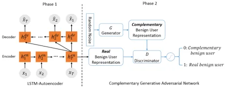
We develop one-class adversarial nets (OCAN) for fraud detection. During training, OCAN contains two phases. First, OCAN adopts the LSTM-Autoencoder (Srivastava, Mansimov, and Salakhutdinov 2015) to encode the benign users into a hidden space based on their online activities, and the encoded vectors are called benign user representa-tions. Then, OCAN trains improved generative adversarial nets in which the discriminator is trained to be a classifier for distinguishing benign users and malicious users with the generator producing potential malicious users. To this end, we adopt the idea of bad GAN (Dai et al. 2017) that the gen-erator is trained to generate complementary samples instead of matching the original data distribution. The generator of the complementary GAN aims to generate samples that are complementary to the representations of benign users, i.e., the potential malicious users. We revise the objective func-tion of the discriminator in the regular GAN to achieve one-class one-classification. The discriminator is trained to separate benign users and complementary samples. Since the behav-iors of malicious users and that of benign users are com-plementary, we expect the discriminator can distinguish be-nign users and malicious users. By combining the encoder of LSTM-Autoencoder and the discriminator of the comple-mentary GAN, OCAN can accurately predict whether a new user is benign or malicious based on his online activities.
separate malicious users from benign users. Third, OCAN can capture the sequential information of user activities. Af-ter training, the detection model can adaptively update a user representation once the user commits a new action and pre-dict whether the user is a fraud or not dynamically.
Related Work
Fraud detection: Many fraud detection techniques have been developed in recent years (Akoglu, Tong, and Koutra 2015; Jiang et al. 2014; Cao et al. 2014; Ying, Wu, and Barbar´a 2011; Kumar and Shah 2018), including based approaches and graph-based approaches. The content-based approaches extract content features, (i.e., text, URL), to identify malicious users from user activities on social networks (Benevenuto et al. 2010). Research in (Kumar, Spezzano, and Subrahmanian 2015) focused on predicting whether a Wikipedia user is a vandal by identifying a set of behavior features based on user edit-patterns. To improve detection accuracy and avoid manual feature construction, a multi-source long-short term memory network (M-LSTM) was proposed to detect vandals (Yuan et al. 2017b). Mean-while, graph-based approaches identify frauds based on net-work topologies. Often based on unsupervised learning, the graph-based approaches consider fraud as anomalies and ex-tract various graph features associated with nodes, edges, ego-net, or communities from the graph (Akoglu, Tong, and Koutra 2015; Manzoor et al. 2016; Ying, Wu, and Barbar´a 2011; Wu et al. 2013).
One-class classification:One-class classification (OCC) al-gorithms aim to build classification models when only one class of samples are observed and the other class of samples are absent (Khan and Madden 2014), which is also related to the novelty detection (Pimentel et al. 2014). One-class sup-port vector machine (OCSVM), as one of widely adopted for one class classification, aims to separate one class of samples from all the others by constructing a hyper-sphere around the observed data samples (Tax and Duin 2004; Manevitz and Yousef 2001). Other traditional classification models also extend to the one-class scenario. For example, one-class nearest neighbor (OCNN) (Tax and Duin 2001) predicts the class of a sample based on its distance to its nearest neighbor in the training dataset. One-class Gaus-sian process (OCGP) chooses a proper GP prior and derives membership scores for one-class classification (Kemmler et al. 2013). However, OCNN and OCGP need to set a thresh-old to detect another class of data. The threshthresh-old is either set by a domain expert or tuned based on a small set of two-class labeled data. In this work, we propose a framework that combines LSTM-Autoencoder and GAN to detect vandals with only knowing benign users. To our best knowledge, this is the first work that examines the use of deep learning mod-els for fraud detection when only one-class training data is available. Meanwhile, comparing to existing one-class al-gorithms, our model trains a classifier by generating a large number of “novel” data and does not require any labeled data to tune parameters.
Preliminary:Generative Adversarial Nets
Generative adversarial nets (GAN) are generative models that consist of two components: a generator G and a dis-criminatorD. Typically, bothGandDare multilayer neural networks. G(z)generates fake samples from a priorpz on
a noise variablezand learns a generative distributionpGto
match the real data distribution pdata. On the contrary, the
discriminative model D is a binary classifier that predicts whether an input is a real data xor a generated fake data fromG(z). Hence, the objective function ofDis defined as:
max
D Ex∼pdata[logD(x)]+Ez∼pz[log(1−D(G(z)))], (1)
where D(·) outputs the probability that · is from the real data rather than the generated fake data. In order to make the generative distributionpG close to the real data distribution
pdata,Gis trained by fooling the discriminator not be able to
distinguish the generated data from the real data. Thus, the objective function ofGis defined as:
min
G Ez∼pz[log(1−D(G(z)))]. (2)
Minimizing the Equation 2 is achieved if the discriminator is fooled by generated dataG(z)and predicts high probability thatG(z)is real data.
Overall, GAN is formalized as a minimax game
min
G maxD V(G, D)with the value function:
V(G, D) =Ex∼pdata[logD(x)]+Ez∼pz[log(1−D(G(z)))].
(3)
Figure 1: The training framework of OCAN
OCAN: One-Class Adversarial Nets
Framework Overview
deployed for fraud detection, is expected to map the benign users and malicious users to relatively separate regions in the continuous feature space because the activity sequences of benign and malicious users are different.
Given the user representations, the second phase is to train a complementary GAN with a discriminator that can clearly distinguish the benign and malicious users. The generator of the complementary GAN aims to generate complemen-tary samples that are in the low-density area of benign users, and the discriminator aims to separate the real and comple-mentary benign users. The discriminator then has the ability to detect malicious users which locate in separate regions from benign users. The framework of training complemen-tary GAN is shown in the right side of Figure 1.
The pseudo-code of training OCAN is shown in Algo-rithm 1. Given a training datasetMbenignthat contains
activ-ity sequence feature vectors ofNbenign users, we first train the LSTM-Autoencoder model (Lines 3–9). After training the Autoencoder, we adopt the encoder in the LSTM-Autoencoder model to compute the benign user representa-tion (Lines 11–14). Finally, we use the benign user repre-sentation to train the complementary GAN (Lines 16–20). For simplicity, we write the algorithm with a minibatch size of 1, i.e., iterating each user in the training dataset to train LSTM-Autoencoder and GAN. In practice, we sample m
real benign users and use the generator to generatem com-plementary samples in a minibatch. In our experiments, the size of minibatch is 32.
Our OCAN moves beyond the naive approach of adopting a regular GAN model in the second phase. The generator of a regular GAN aims to generate the representations of fake benign users that are close to the representations of real be-nign users. The discriminator of a regular GAN is to identify whether an input is a representation of a real benign user or a fake benign user from the generator. However, one potential drawback of the regular GAN is that once the discriminator is converged, the discriminator cannot have high confidence on separating real benign users from real malicious users. We denote the OCAN with the regular GAN as OCAN-r and compare its performance with OCAN in the experiment.
LSTM-Autoencoder for User Representation
The first phase of OCAN is to encode users to a continu-ous hidden space. Since each online user has a sequence of activities (e.g., edit a sequence of pages), we adopt LSTM-Autoencoder to transform a variable-length user activity se-quence into a fixed-dimension user representation. Formally, given a useruwithTactivities, we represent the activity se-quence asXu= (x1, . . . ,xt, . . . ,xT)wherext∈Rdis the t-th activity feature vector.
Encoder:The encoder encodes the user activity sequence Xuto a user representation with an LSTM model:
hent =LST Men(xt,hent−1), (4)
wherextis the feature vector of thet-th activity;hent
indi-cates thet-th hidden vector of the encoder. The last hidden vectorhen
T captures the information of a
whole user activity sequence and is considered as the user
Algorithm 1:Training One-Class Adversarial Nets
Inputs :Training datasetMbenign={X1,· · ·,XN},
Training epochs for LSTM-Autoencoder
EpochAEand GANEpochGAN Outputs:Well-trained LSTM-Autoencoder and
complementary GAN
1 initialize parameters in LSTM-Autoencoder and complementary GAN;
2 j←0;
3 whilej < EpochAEdo 4 foreachuseruinMbenigndo
5 compute the reconstructed sequence of user activities by LSTM-Autoencoder (Eq. 4, 6, and 7);
6 optimize the parameters in LSTM-Autoencoder with the loss function Eq. 8;
7 end 8 j←j+ 1; 9 end
10 V=∅;
11 foreachuseruinMbenigndo
12 compute the benign user representationvuby the
encoder of LSTM-Autoencoder (Eq. 4, 5); 13 V+ =vu;
14 end 15 j←0;
16 whilej < EpochGANdo
17 foreachbenign user representationvuinVdo
18 optimize the discriminatorDand generatorGwith loss functions Eq. 14, 12, respectively;
19 end 20 end
21 returnwell-trained LSTM-Autoencoder and complementary GAN
representationv:
v=henT . (5) Decoder:In our model, the decoder adopts the user rep-resentation v as the input to reconstruct the original user activity sequenceX:
hdet =LST Mde(v,hdet−1), (6)
ˆ
xt=f(hdet ), (7)
wherehdet is the t-th hidden vector of the decoder;xˆt
in-dicates the t-th reconstructed activity feature vector; f(·)
denotes a neural network to compute the sequence outputs from hidden vectors of the decoder. Note that we adopt v
as input of the whole sequence of the decoder, which has achieved great performance on sequence-to-sequence mod-els (Cho et al. 2014).
The objective function of LSTM-Autoencoder is:
L(AE)(ˆxt,xt) = T
X
t=1
(ˆxt−xt)2, (8)
wherext(xˆt) is thet-th (reconstructed) activity feature
vec-tor. After training, the last hidden vector of encoderhT can
reconstruct the sequence of user feature vectors. Thus, the representation of userv=hen
T captures the salient
Complementary GAN
The generatorGof complementary GAN is the same as that of the bad GAN in (Dai et al. 2017). Basically, it is a feed-forward neural network where its output layer has the same dimension as the user representationv. Formally, we define the generated samples as v˜ = G(z). Unlike the generator in a regular GAN which is trained to match the distribution of the generated fake benign user representation with that of benign user representationpdata, the generatorGof
com-plementary GAN learns a generative distributionpG that is
close to the complementary distribution p∗ of the benign user representations, i.e.,pG=p∗.
Following (Dai et al. 2017), we define the complementary distribution p* as:
p∗(˜v) = (1
τ
1
pdata(˜v) ifpdata(˜v)> andv˜ ∈ Bv C ifpdata(˜v)≤andv˜ ∈ Bv,
(9)
whereis a threshold to indicate whether the generated sam-ples are in high-density regions;τ is a normalization term;
Cis a small constant;Bvis the space of user representation.
To make the generative distributionpG close to the
com-plementary distributionp∗, the complementary generatorG
is trained to minimize the KL divergence betweenpG and
p∗. Based on the definition of KL divergence, the objective function is:
LKL(pGkp∗)=−H(pG)−Ev˜∼pGlogp
∗(˜v)
=−H(pG) +Ev˜∼pGlogpdata(˜v)1[pdata(˜v)> ] +E˜v∼pG(1[pdata(v˜)> ] logτ−1[pdata(˜v)≤] logC),
(10)
whereH(·)is the entropy, and1[·]is the indicator function. The last term of Equation 10 can be omitted because bothτ
andCare constant terms and the gradients of the indicator function1[·]with respect to parameters of the generator are mostly zero.
Meanwhile, following (Dai et al. 2017), the complemen-tary generatorGadopts the feature matching loss (Salimans et al. 2016) to ensure that the generated samples are con-strained in the space of user representationBv.
Lfm=kEv˜∼pGf(˜v)−Ev∼pdataf(v)k
2
2, (11)
wheref(·)denotes the output of an intermediate layer of the discriminator used as a feature representation ofv.
Thus, the complete objective function of the generator is defined as:
min
G − H(pG) +Ev˜∼pGlogpdata(˜v)1[pdata(˜v)> ]
+kEv˜∼pGf(˜v)−Ev∼pdataf(v)k
2 2.
(12)
Overall, the objective function of the complementary gen-erator aims to let the generative distributionpGclose to the
complementary samples p∗, i.e., pG = p∗, and make the
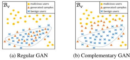
generated samples from different regions (but in the same space of user representations) than those of the benign users. Figure 2 illustrates the difference of the generators of reg-ular GAN and complementary GAN. The objective function
of the generator of regular GAN in Equation 2 is trained to fool the discriminator by generating fake benign users sim-ilar to the real benign users. Hence, as shown in Figure 2a, the generator of regular GAN generates the distribution of fake benign users that have the similar distribution of real benign users in the feature space. On the contrary, the ob-jective function of the generator of complementary GAN in Equation 12 is trained to generate complementary samples that are in the low-density regions of benign users (shown in Figure 2b).
(a) Regular GAN (b) Complementary GAN
Figure 2: Demonstrations of the ideal generators of regular GAN and complementary GAN. The blue dot line indicates the high density regions of benign users.
To optimize the objective function of generator, we need to approximate the entropy of generated samplesH(pG)and
the probability distribution of real samples pdata. To
min-imize −H(pG), following (Dai et al. 2017), we adopt the
pull-away term (PT) proposed by (Zhao, Mathieu, and Le-Cun 2016) that encourages the generated feature vectors to be orthogonal. The PT term increases the diversity of gener-ated samples and can be considered as a proxy for minimiz-ing−H(pG). The PT term is defined as
LP T =
1 N(N−1)
N
X
i N
X
j6=i
( f(˜vi)
Tf(˜v j)
kf(˜vi)kkf(˜vj)k
)2, (13)
whereN is the size of a mini-batch.
The probability distribution of real samplespdata is
usu-ally unavailable, and approximatingpdatais computationally
expensive. In this paper, we adopt the approach proposed by (Schoneveld 2017) that a discriminator from a regular GAN can detect whether the data from the real data distribution
pdata or from the generator’s distribution. The basic idea is
that the discriminator is able to detect whether a sample is from the real data distribution pdata or from the generator
when the generator is trained to generate samples that are close to real benign users. Hence, the discriminator is suf-ficient to identify the data points that are above a thresh-old of pdata during training. We separately train a regular
GAN model based on benign user representations and use the discriminator of the regular GAN as a proxy to evaluate
pdata(˜v)> .
The discriminatorDtakes the benign user representation
layer, and we define the objective function ofDas:
max
D Ev∼pdata[logD(v)] +Ev˜∼pG[log(1−D(˜v))]+ Ev∼pdata[D(v) logD(v)].
(14)
Different from the objective function of the discriminator in-troduced in the bad GAN for the purpose of semi-supervised learning, we revise the objective function of D in our com-plementary GAN based on the regular GAN. The first two terms in Equation 14 are the objective function of discrimi-nator in the regular GAN model. Therefore, the discrimina-tor of complementary GAN is trained to separate the benign users and complementary samples. The last term in Equation 14 is a conditional entropy term which encourages the dis-criminator to detect real benign users with high confidence. Then, the discriminator is able to separate the benign and malicious users clearly.
Although the objective functions of the discriminators of regular GAN and complementary GAN are similar, the ca-pabilities of discriminators of regular GAN and complemen-tary GAN for malicious detection are different. The discrim-inator of regular GAN aims to separate the benign users and generated fake benign users. However, after training, the generated fake benign users locate in the same regions as the real benign users (shown in Figure 2a). The probabilities of real and generated fake benign users predicted by the dis-criminator of regular GAN are all close to 0.5. Thus, giving a benign user, the discriminator cannot predict the benign user with high confidence. On the contrary, the discrimina-tor of complementary GAN is trained to separate the benign users and generated complementary samples. Since the gen-erated complementary samples have the same distribution as the malicious users (shown in Figure 2b), the discriminator of complementary GAN can also detect the malicious users.
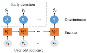
Figure 3: The fraud detection model
Fraud Detection Model
Although the training procedure of OCAN contains two phases that train LSTM-Autoencoder and complementary GAN successively, the fraud detection model is an end-to-end model. We illustrate its structure in Figure 3. To de-tect a malicious user, we first compute the user represen-tationvu based on the encoder in the LSTM-Autoencoder
model (Equations 4 and 5). Then, we predict the user la-bel based on the discriminator of complementary GAN, i.e.,
p(ˆyu|vu) =D(vu).
Early fraud detection: The upper-left region of Figure 3 shows that our OCAN model can also achieve early de-tection of malicious users. Given a useru, at each stept, the hidden stateshen
utare updated until thet-th step by taking the
current feature vectorxutas input and are able to capture the
user behavior information until thet-th step. Thus, the user representation at thet-th step is denoted asvut =h
en ut.
Fi-nally, we can use the discriminatorDto calculate the prob-abilityp(ˆyut|vut) =D(vut)of the user to be a malicious
user based on the current step user representationvt.
Experiments
Experiment Setup
Dataset:To evaluate OCAN, we focus on one type of mali-cious users, i.e., vandals on Wikipedia. We conduct our eval-uation on UMDWikipedia dataset (Kumar, Spezzano, and Subrahmanian 2015). This dataset contains information of around 770K edits from Jan 2013 to July 2014 (19 months) with 17105 vandals and 17105 benign users. Each user edits a sequence of Wikipedia pages. We keep those users with the lengths of edit sequence range from 4 to 50. After this preprocessing, the dataset contains 10528 benign users and 11495 vandals.
To compose the feature vectorxt of the user’st-th edit,
we adopt the following edit features: (1) whether or not the user edited on a meta-page; (2) whether or not the user con-secutively edited the pages less than 1 minutes; (3) whether or not the user’s current edit page had been edited before; (4) whether or not the user’s current edit would be reverted.
Hyperparameters:For LSTM-Autoencoder, the dimension of the hidden layer is 200, and the training epoch is 20. For the complementary GAN model, both discriminator and generator are feedforward neural networks. Specifically, the discriminator contains 2 hidden layers which are 100 and 50 dimensions. The generator takes the 50 dimensions of noise as input, and there is one hidden layer with 100 dimensions. The output layer of the generator has the same dimension as the user representation which is 200 in our experiments. The training epoch of complementary GAN is 50. The threshold
defined in Equation 12 is set as the 5-quantile probability of real benign users predicted by a pre-trained discriminator. We evaluated several values from 4-quantile to 10-quantile and found the results are not sensitive.
Repeatability: Our software together with the datasets are available at https://github.com/PanpanZheng/OCAN.
Comparison with One-Class Classification
Baselines: We compare OCAN with the following widely used one-class classification approaches:
• One-class nearest neighbors (OCNN) (Tax and Duin 2001) labels a testing sample based on the distance from the sample to its nearest neighbors in training dataset and the average distance of those nearest neighbors.
Table 1: Vandal detection results (mean±std.) on precision, recall, F1 and accuracy
Input Algorithm Precision Recall F1 Accuracy
Raw feature vector
OCNN 0.5680±0.0129 0.8646±0.0599 0.6845±0.0184 0.6027±0.0161
OCGP 0.5767±0.0087 0.9000±0.0560 0.7023±0.0193 0.6196±0.0142
OCSVM 0.6631±0.0057 0.9829±0.0011 0.7919±0.0040 0.7417±0.0064
User representation
OCNN 0.8314±0.0351 0.8028±0.0476 0.8150±0.0163 0.8181±0.0153
OCGP 0.8381±,0.0225 0.8289±0.0374 0.8326±0.0158 0.8337±0.0139
OCSVM 0.6558±0.0058 0.9590±0.0096 0.7789±0.0064 0.7278±0.0080
OCAN 0.9067±0.0615 0.9292±0.0348 0.9010±0.0228 0.8973±0.0244
User representation OCAN-r 0.8673±0.0355 0.8759±0.0529 0.8701±0.0267 0.8697±0.0244
• One-class SVM (OCSVM) (Tax and Duin 2004) adopts support vector machine to learn a decision hypersphere around the positive data, and considers samples located outside this hypersphere as anomalies.
For baslines, we use the implementation provided in ND-tool2. The hyperparameters of baselines set as default values
in NDtool. Note that both OCNN and OCGP require a small portion (5% in our experiments) of vandals as a validation dataset to tune an appropriate threshold for vandal detection. However, OCAN does not require any vandals for training and validation. Since the baselines are not sequence models, we compare OCAN to baselines in two ways. First, we con-catenate all the edit feature vectors of a user to araw feature vector as an input to baselines. Second, the baselines have the same inputs as the discriminator, i.e., theuser represen-tationvcomputed from the encoder of LSTM-Autoencoder. Meanwhile, OCAN cannot adopt the raw feature vectors as inputs to detect vandals. This is because GAN is only suit-able for real-valued data (Goodfellow et al. 2014).
To evaluate the performance of vandal detection, we ran-domly select 7000 benign users as the training dataset and 3000 benign users and 3000 vandals as the testing dataset. We report the mean value and standard deviation based on 10 different runs. Table 1 shows the means and standard de-viations of the precision, recall, F1 score and accuracy for vandal detection. First, OCAN achieves better performances than baselines in terms of F1 score and accuracy in both in-put settings. It means the discriminator of complementary GAN can be used as a one-class classifier for vandal detec-tion. We can further observe that when the baselines adopt the raw feature vector instead of user representation, the per-formances of both OCNN and OCGP decrease significantly. It indicates that the user representations computed by the encoder of LSTM-Autoencoder capture the salient informa-tion about user behavior and can improve the performance of one-class classifiers. However, we also notice that the stan-dard deviations of OCAN are higher than the baselines with user representations as inputs. We argue that this is because GAN is widely known for difficult to train. Thus, the stabil-ity of OCAN is relatively lower than the baselines.
Furthermore, we show the experimental results of OCAN-r, which adopts the regular GAN model instead of the com-plementary GAN in the second training phase of OCAN, in the last row of Table 1. We can observe that the performance
2
http://www.robots.ox.ac.uk/∼davidc/publications NDtool.php
of OCAN is better than OCAN-r. It indicates that the dis-criminator of complementary GAN which is trained on real and complementary samples can more accurately separate the benign users and vandals.
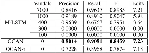
Table 2: Early detection results on precision, recall, F1, and the average number of edits before the vandals are blocked
Vandals Precision Recall F1 Edits
M-LSTM
7000 0.8416 0.9637 0.8985 7.21 1000 0.9189 0.8910 0.9047 5.98 400 0.9639 0.6767 0.7951 3.64 300 0.0000 0.0000 0.0000 0.00 100 0.0000 0.0000 0.0000 0.00
OCAN 0 0.8014 0.9081 0.8459 7.23
OCAN-r 0 0.7228 0.8968 0.7874 7.18
Comparison with M-LSTM for Early Vandal
Detection
We further compare the performance of OCAN in terms of early vandal detection with one latest deep learning based vandal detection model, M-LSTM, developed in (Yuan et al. 2017b). Note that M-LSTM assumes a training dataset that contains both vandals and benign users. In our experiments, we train our OCAN with the training data consisting of 7000 benign users and no vandals and train M-LSTM with a train-ing data consisttrain-ing the same 7000 benign users and a varytrain-ing number of vandals (from 7000 to 100). For OCAN and M-LSTM, we use the same testing dataset that contains 3000 benign users and 3000 vandals. Note that in OCAN and M-LSTM, the hidden statehen
t of the LSTM model captures
the up-to-date user behavior information and hence we can achieve early vandal detection. The difference is that the M-LSTM model uses hent as the input of a classifier directly whereas OCAN further trains complementary GAN and uses its discriminator as a classifier to make the early vandal de-tection. In this experiment, instead of applying the classifier on the final user representationv = henT , the classifiers of M-LSTM and OCAN are applied on each step of LSTM hid-den statehen
t and predict whether a user is a vandal after the
user commits the t-th action.
(a) Prob. predicted by OCAN (b) Prob. predicted by OCAN-r (c) F1 score of OCAN (d) F1 score of OCAN-r
Figure 4: Training progresses of OCAN (4a,4c) and OCAN-r(4b,4d). Three lines in Figures 4a and 4b indicate the probabilities of benign users predicted by the discriminator: real benign usersp(y|vB)(green line) vs. generated samplesp(y|v˜)(red broken
line) vs. real malicious usersp(y|vM)(blue dotted line). Figures 4c and 4d show the F1 of OCAN and OCAN-r during training.
as the M-LSTM when the number of vandals in the training dataset is large (1000, 4000, and 7000). However, M-LSTM has very poor accuracy when the number of vandals in the training dataset is small. In fact, we observe that M-LSTM could not detect any vandal when the training dataset con-tains less than 400 vandals. On the contrary, OCAN does not need any vandal in the training data.
The experimental results of OCAN-r for early vandal de-tection are shown in the last row of Table 2. OCAN-r outper-forms M-LSTM when M-LSTM is trained on a small num-ber of the training dataset. However, the OCAN-r is not as good as OCAN. It indicates that generating complementary samples to train the discriminator can improve the perfor-mance of the discriminator for vandal detection.
OCAN Framework Analysis
Complementary GAN vs. Regular GAN: In our OCAN model, the generator of complementary GAN aims to gener-ate complementary samples that lie in the low-density region of real samples, and the discriminator is trained to detect the real and complementary samples. We examine the training progress of OCAN in terms of predication accuracy. We cal-culate probabilities of real benign usersp(y|vB)(shown as
green line in Figure 4a), malicious usersp(y|vM)(blue
dot-ted line) and generadot-ted samplesp(y|˜v)(read broken line) being benign users predicted by the discriminator of com-plementary GAN on the testing dataset after each training epoch. We can observe that after OCAN is converged, the probabilities of malicious users predicted by the discrimina-tor of complementary GAN are much lower than that of be-nign users. For example, at the epoch 40, the average prob-ability of real benign usersp(y|vB)predicted by OCAN is
around70%, while that of malicious usersp(y|vM)is only
around30%. Meanwhile, the average probability of gener-ated complementary samplesp(y|v˜)lies between the prob-abilities of benign and malicious users.
On the contrary, the generator of a regular GAN in the OCAN-r model generates fake samples that are close to real samples, and the discriminator of GAN focuses on distin-guishing the real and generated fake samples. As shown in Figure 4b, the probabilities of real benign users and prob-abilities of malicious users predicted by the discriminator of regular GAN become close to each other during train-ing. After the OCAN-r is converged, both the probabilities
of real benign users and malicious users are close to 0.5. Meanwhile, the probability of generated samples is similar to the probabilities of real benign users and malicious users. We also show the F1 scores of OCAN and OCAN-r on the testing dataset after each training epoch in Figure 4c and 4d. We can observe that the F1 score of OCAN-r is not as stable as (and also a bit lower than) OCAN. This is because the outputs of the discriminator for real and fake samples are close to 0.5 after the regular GAN is converged. If the proba-bilities of real benign users predicted by the discriminator of the regular GAN swing around 0.5, the accuracy of vandal detection will fluctuate accordingly.
We can observe from Figure 4 another nice property of OCAN compared with OCAN-r for fraud detection, i.e., OCAN is converged faster than OCAN-r. We can observe that OCAN is converged with only training 20 epochs while the OCAN-r requires nearly 100 epochs to keep stable. This is because the complementary GAN is trained to separate the benign and malicious users while the regular GAN mainly aims to generate fake samples that match the real samples. In general, matching two distributions requires more train-ing epochs than separattrain-ing two distributions. Meanwhile, the feature matching term adopted in the generator of comple-mentary GAN is also able to improve the training process (Salimans et al. 2016).
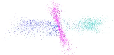
Figure 5: 2D visualization of three types of users: real be-nign (blue star), vandal (cyan triangle), and complementary benign (red dot)
Langford 2000) and show the projection in Figure 5. We ob-serve that the generated complementary users lie in the low-density regions of real benign users. Meanwhile, the gen-erated samples are also between the benign users and van-dals. Since the discriminator is trained to separate the benign and complementary benign users, the discriminator is able to separate benign users and vandals.
Conclusion
In this paper, we have developed OCAN for fraud detec-tion when only benign users are available during the training phase. During training, OCAN adopts LSTM-Autoencoder to learn benign user representations, and then uses the be-nign user representations to train a complementary GAN model. The generator of complementary GAN can gener-ate complementary benign user representations that are in the low-density regions of real benign user representations, while the discriminator is trained to distinguish the real and complementary benign users. After training, the discrimina-tor is able to detect malicious users which are outside the regions of benign users. We have conducted theoretical and empirical analysis to demonstrate the advantages of com-plementary GAN over regular GAN. We conducted experi-ments on a real world dataset and showed that OCAN out-performs the state-of-the-art one-class classification models.
Acknowledgments
This work was supported in part by NSF 1564250, 1564348, 1564039 and 1841119.
References
Akoglu, L.; Tong, H.; and Koutra, D. 2015. Graph based anomaly detection and description: a survey. DMKD
29(3):626–688.
Benevenuto, F.; Magno, G.; Rodrigues, T.; and Almeida, V. 2010. Detecting spammers on twitter. InCEAS.
Cao, Q.; Yang, X.; Yu, J.; and Palow, C. 2014. Uncovering large groups of active malicious accounts in online social networks. InCCS.
Cheng, J.; Bernstein, M.; Danescu-Niculescu-Mizil, C.; and Leskovec, J. 2017. Anyone can become a troll: Causes of trolling behavior in online discussions. In CSCW, 1217– 1230.
Cho, K.; van Merrienboer, B.; Gulcehre, C.; Bahdanau, D.; Bougares, F.; Schwenk, H.; and Bengio, Y. 2014. Learning phrase representations using rnn encoder-decoder for statis-tical machine translation.arXiv:1406.1078 [cs, stat]. Dai, Z.; Yang, Z.; Yang, F.; Cohen, W. W.; and Salakhutdi-nov, R. 2017. Good semi-supervised learning that requires a bad gan. InNIPS.
Goodfellow, I. J.; Pouget-Abadie, J.; Mirza, M.; Xu, B.; Warde-Farley, D.; Ozair, S.; Courville, A.; and Bengio, Y. 2014. Generative adversarial networks. InNIPS.
Jiang, M.; Cui, P.; Beutel, A.; Faloutsos, C.; and Yang, S. 2014. Catchsync: Catching synchronized behavior in large directed graphs. InKDD.
Kemmler, M.; Rodner, E.; Wacker, E.-S.; and Denzler, J. 2013. One-class classification with gaussian processes. Pat-tern Recognition46(12):3507–3518.
Khan, S. S., and Madden, M. G. 2014. One-class classi-fication: taxonomy of study and review of techniques. The Knowledge Engineering Review29(3):345–374.
Kumar, S., and Shah, N. 2018. False information on web and social media: A survey. arXiv:1804.08559 [cs]. Kumar, S.; Cheng, J.; Leskovec, J.; and Subrahmanian, V. S. 2017. An army of me: Sockpuppets in online discussion communities. InWWW, 857–866.
Kumar, S.; Spezzano, F.; and Subrahmanian, V. 2015. Vews: A wikipedia vandal early warning system. In KDD, 607– 616.
Manevitz, L. M., and Yousef, M. 2001. One-class svms for document classification. JMLR2(Dec):139–154.
Manzoor, E. A.; Momeni, S.; Venkatakrishnan, V. N.; and Akoglu, L. 2016. Fast memory-efficient anomaly detection in streaming heterogeneous graphs. InKDD.
Pimentel, M. A. F.; Clifton, D. A.; Clifton, L.; and Tarassenko, L. 2014. A review of novelty detection. Signal Processing99:215–249.
Radford, A.; Metz, L.; and Chintala, S. 2015. Unsupervised representation learning with deep convolutional generative adversarial networks. arXiv:1511.06434 [cs].
Salimans, T.; Goodfellow, I.; Zaremba, W.; Cheung, V.; Rad-ford, A.; and Chen, X. 2016. Improved techniques for train-ing gans. arXiv:1606.03498 [cs].
Schoneveld, L. 2017. Semi-Supervised Learning with Gen-erative Adversarial Networks. Ph.D. Dissertation.
Srivastava, N.; Mansimov, E.; and Salakhutdinov, R. 2015. Unsupervised learning of video representations using lstms. InICML.
Tax, D. M. J., and Duin, R. P. W. 2001. Uniform ob-ject generation for optimizing one-class classifiers. JMLR
2(Dec):155–173.
Tax, D. M. J., and Duin, R. P. W. 2004. Support vector data description. Machine Learning54(1):45–66.
Tenenbaum, J. B.; Silva, V. d.; and Langford, J. C. 2000. A global geometric framework for nonlinear dimensionality reduction. Science290(5500):2319–2323.
Wu, L.; Wu, X.; Lu, A.; and Zhou, Z. 2013. A spectral approach to detecting subtle anomalies in graphs. J. Intell. Inf. Syst.41(2):313–337.
Ying, X.; Wu, X.; and Barbar´a, D. 2011. Spectrum based fraud detection in social networks. InICDE, 912–923. Yuan, S.; Wu, X.; Li, J.; and Lu, A. 2017a. Spectrum-based deep neural networks for fraud detection. InCIKM. Yuan, S.; Zheng, P.; Wu, X.; and Xiang, Y. 2017b. Wikipedia vandal early detection: from user behavior to user embed-ding. InECML/PKDD.