www.adv-radio-sci.net/11/251/2013/ doi:10.5194/ars-11-251-2013
© Author(s) 2013. CC Attribution 3.0 License.
Radio Science
Industrial interference and radio astronomy
A. Jessner
Max-Planck-Institut fuer Radioastronomie, Auf dem Huegel 69, 53121 Bonn, Germany Correspondence to: A. Jessner ([email protected])
Abstract. The interferer – victim scenario is described for the case of industrial interference affecting radio astronom-ical observatories. The sensitivity of radio astronomastronom-ical re-ceivers and their interference limits are outlined. EMC above 30 MHz is a serious problem for Radio Astronomy. Interferer (CISPR) and victim (ITU-R RA 769) standards are not har-monised. The emissions from the interferer and their spec-tral characteristics are not defined sufficiently well by CISPR standards. The required minimum coupling losses (MCL) be-tween an industrial device and radio astronomical antenna depends on device properties but is shown to exceed 140 dB in most cases. Spatial separation of a few km is insufficient on its own, the terrain must shield>30–40 dB, additional mitigations such as extra shielding or suppression of high fre-quency emissions may be necessary. A case by case compat-ibility analysis and tailored EMC measures are required for individual installations. Aggregation of many weak rfi emit-ters can become serious problem. If deployment densities are high enough, the emission constraints can even exceed those for a single interferer at a short distance from the radio ob-servatory. Compatibility studies must account not only for the single interferer but also for many widely distributed in-terference sources.
1 The victim
Radio astronomy installations (observatories) are a large-scale and cost intensive part of the scientific infrastructure that is fully financed by the tax payer. They have to be large and expensive, because the radio signals we receive from cosmic sources are extremely attenuated and one needs large antennas with large collecting areas and sophisticated cryo-genic receivers for their detection. Radio astronomy belongs to the realm of fundamental science. But it has also led to quite a few technical applications (e.g. feed horns for satel-lite dishes), and its techniques are used in vital measurements such as the establishment of a very precise global
coordi-nate system which even accounts for the motion of the con-tinents but these have been serendipitous side effects, which are nevertheless welcome by all. The aim of radio astronomi-cal research is however to understand the structure of the cos-mos we find ourselves in, the development of the universe, its galaxies, stellar systems and planets as well as the very struc-ture of space-time itself. Radio astronomy also plays a sig-nificant role in the education of new scientists and engineers in astrophysics as well as in the fields of radio engineering, image processing, data acquisition and many more. As such it is a long-term investment of society into its own future, something outside the scope of commercial interests that de-mand an identifiable return within a predictable timescale. It is only logical that governments try to protect their invest-ments like anyone else and perhaps for that reason, radio as-tronomy became a recognised radio service within the radio regulations (RR) of the ITU1 (Radio Regulations, 2012), a global set of rules governing the allocation and use of ra-dio spectrum which is updated regularly by the world rara-dio conferences. Radio astronomy is a passive (listen only) radio service detecting natural radio emissions in contrast to most other usage of the radio spectrum that involves technical ra-dio transmitters (active services).
One of the reasons for the unequalled sensitivity of radio astronomical measurements lies in the principle of compar-ing the received radio flux density from an unknown source to that of the know radio background (Dicke, 1946), whereby sensitivities of more than 50dB below the background noise
(S/N <−50 dB) can be achieved. Such sensitive radiometric
measurements are only possible, if the reference sky (back-ground) is free from interference itself, and that to a degree exceeding the most sensitive measurements. As a result, ra-dio astronomy has been allocated specific protected bands, mostly around frequencies where molecules of the tenuous cosmic gases emit their spectral lines (Fig. 1).
1 107 1 108 1 109 1 1010 1 1011 0.1
fr equency (Hz)
i
Fig. 1. The Radio sky temperature (Cane, 1979; Ellington, 2005) and radio astronomical allocations between 10 MHz and 100 GHz. Red:
Sky temperature for the Zenith, green: passive bands allocated to radio astronomy, blue: bands shared with other services.
Radio astronomy has an exclusive use of only 0.7 % of the radio spectrum below 30 GHz, the majority of the allo-cated bands are shared with other radio services. The choice of these bands is not free and neither is that of the interfer-ence thresholds. Both are determined by the physics of the distant emitter and the physical limits of a radio receiver and its use in sensitive radio astronomical measurements. Exclu-sive bands for radio astronomy are covered by the RR Foot-note 5.340 (Radio Regulations, 2012) which says that “no emissions are permitted in a list of bands” with emissions being termed as radiation coming from a radio station (of any kind) as the result of its active operation. Radiation from other parts of the station, e.g. the local oscillator or the IF of a receiver is not an emission in that sense, an important distinction as we will see later on.
The ITU Recommendation RA 769 (ITU-R, 2003) lists the specific threshold levels of radio interference for which the interference becomes detrimental to the operation of the ra-dio observatory. These levels are specified as 10 dB below the radiometric receiver sensitivity, typically an I/N of−60 dB, implying that measurement results should not be affected by an additional error of more than 10 %.
Radio astronomical antennas have forward gains depend-ing on frequency, but typically of the order of 50–60 dBi within a narrow beam of a width of typically a few minutes of arc. Interference enters the receiver mainly via sidelobes with varying degrees of gain or attenuation. For interference estimates the radio astronomical receiver is assumed to have an average gain of 0 dBi for reception from random direc-tions. Measurement errors of radiometric noise power mea-surements decrease with the square root of the product of band width and averaging time (Dicke, 1946) requiring an appropriate scaling of interference thresholds. As a result of these considerations, the interference thresholds are given by Eq. (1)
SH=0.1·4π k f
2·(T
ant+Trec)
c2√1f τ (1)
0.01 0.1 1 10 100 1103
260 240 220 200 180
Frequency GHz
S
PF
D
[dB
W
/
(m
^2
.H
z)]
Fig. 2. Detrimental spectral flux density values for radio astronomy
according to ITU-R RA 769. Black: continuum limit, red: spectro-scopic limit.
taken from ITU-R RA 769. As usual, k is the Boltzmann constant andcthe speed of light. The resultSH is the
spec-tral flux density threshold (W m−2Hz−1), withf being the centre frequency of the band,Tant the typical antenna
tem-perature andTrec the typical receiver temperature,1f is the
measurement bandwidth andτ the duration of the signal in-tegration. ITU-R RA 769 lists these quantities in its Tables 1 and 2 for continuum (broad band) and spectroscopy (nar-row band) measurements. Figure 2 shows the thresholds as a function of frequency for an integration time of 2000 s.
The interference limits are defined for the victim in the case of radio astronomy as averages over time and band-width.
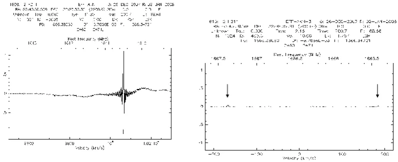
Fig. 3. Interference received from a low earth orbit mobile phone satellite (right) and a typical cosmic radio source (two small bumps in the
left panel) at 1610 GHz (diagrams courtesy of A. Kraus).
A few numbers may serve to illustrate the magnitude of the quantities and of the achieved sensitivities: one Jy is the spec-tral flux density that one would receive on the ground from a 1 W e.i.r.p IMT-2000 mobile phone operating at 2.1 GHz and orbiting the earth at a distance of 8.867×10⁵km, more than twice the distance to the moon! The main beam sensitivity of a large radio telescope at that frequency can exceed 50 dBi. If we assume a 10 MHz detection bandwidth, the 100 m Ef-felsberg radio telescope is capable of detecting such a 1 W e.i.r.p. source at a distance of 6.9×10⁷km after 2000 s. In
this case we receive a spectral flux density of 0.17 mJy, which is a typical strength of the signals received from distant cos-mic sources. Figure 3 illustrates the difference between the signals strengths of interference and a cosmic source.
The interference source was one of the IRIDIUM global mobile phone satellites at a distance of 1500 km. They em-ploy a spot beam with a peak e.i.r.p. of 12.5 W and our mea-surements have shown that their seventh-order intermodula-tion products with an e.i.r.p. of 1 mW (ECC Rep. 171, 2011; ECC Doc. SE40(09)092, 2009) are causing the interference even when the satellite is not crossing the telescope beam.
Radio observatories are also vulnerable to regular and ir-regular impulsive interference. When they observe Pulsars, a class of radio sources that emits short radio pulses with pe-riods ranging from 1.5 ms to more than eight seconds, they employ sensitive high time resolution detectors. Simple elec-tric cattle fences in about two km distance from the telescope have frequently been detected as regular pulsed interference. It becomes clear, that local radio emissions, even those that are considered weak by normal standards can become the source of severe interference for a radio observatory. This is particularly true, when the emission occurs within the radio astronomical bands. Frequency regulators have recognised the problem and implemented a complex set of protection measures for radio astronomy, based on extensive studies that
investigated the compatibility of radio astronomy with active radio services.
2 Industrial interference
The ITU came into being because there was a need to co-ordinate the frequencies and locations of radio transmitters world-wide, for radio waves can travel far and by them-selves do not respect conventions such as national bound-aries. Hence the focus on ITU regulations is on transmis-sions intended for communication and information transfer in the widest possible sense. That includes not only broad-casting, radio amateurs, location tracking (radar), but also remote sensing and radio astronomy.
Fig. 4. Contributions to the radio noise environment (from ITU-R
P. 372-9, 2007).
from localised concentrations of fixed installations in cities and industrial areas by their distance to the radio observatory and the terrain.
However with the increased use of high speed digital de-vices contained in license exempt and uncontrolled and often mobile consumer electronics as well as the spread of effi-cient high speed switching gear in consumer and industrial power conversion equipment, ranging from simple switch mode power supplies for a laptop to MW-size generators and converters in wind power plant, brings the sources of indus-trial interference closer to the radio observatories. Not only that, their interference spectrum will also be broader as it is naturally related to the rise and fall times of the digital switching used and these have become much faster with the recent advances in semiconductor electronics.
Standards are needed to limit the emission from such de-vices in order to suppress interference to communication equipment and also to other sensitive electrical equipment. These have been devised by CISPR2 for a range of equip-ment separated into different categories and classes accord-ing to their use and construction. A list is given in the CISPR guide of the IEC (IEC, 2007). There two main classes:
1. equipment intended for use in a commercial and/or light industrial environment,
2. equipment intended for domestic use.
Class B equipment has to fulfil more stringent requirements than that from class A.
2Comit´e International Sp´ecial des Perturbations
Ra-dio´electriques, the “special international committee on radio interference” is part of the international electro-technical commis-sion (IEC).
become common not only in the city but also in the rural environment close to radio observatories. The new scenario requires a detailed study of the impact of new industrial de-vices on radio astronomical measurements. In this paper we will look at the example of industrial switch-mode power converters in the kW to MW range which are often found in association with wind power generators or solar power stations. Like radio observatories, these are also erected in remote areas in order to avoid densely populated areas3.
The radio disturbance characteristics and limits are given as field strengths at a distance of 30 m in table 17 of the Eu-ropean standard CISPR-11 (=EN DIN 55011 in Germany) for such devices belonging to group 1 class A:
30 dB µV m−1forf <230 MHz and 120 kHz measure-ment bandwidth
37 dB µV m−1 for 230 MHz< f <1 GHz and 1 MHz
measurement bandwidth
No limits are prescribed for f >1 GHz and we will therefore continue to use the limit of
37 dBµV m−1for allf >1 GHz
A quasi peak detector is to be used for the measurements and no further specification of the spectrum apart from mea-surement bandwidth has been made. Many devices may emit narrow band radiation in the form of harmonics of their prin-cipal operating frequency, with a spacing that corresponds to the fundamental clock frequency. Radio astronomical bands are several MHz to several tens of MHz wide and power-ful switches with switching rates of the order of a few ten kHz will create many harmonics within a radio astronomi-cal band, creating an interference that often approximates a broad band signal.
However the increasing complexity and sophistication of the control and electronics of such devices, may also result in broad band interference, e.g. when switching frequencies and duty cycles vary on short timescales. Specifying peak or quasi-peak values only, makes the duration of the interfer-ence uncertain, it could last only for a few ms or for many
3This document should however not be interpreted as one of
10 100 1 103 1 104 1 105 250
200 150 100 50 0
MHz
P
(
dB
W
)
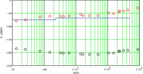
Fig. 5. Emission and reception power limits as specified by
CISPR-11 and ITU-R RA 769. The blue trace is the e.i.r.p. per measurement channel as given by CISPR-11, the red diamonds indicate the max-imum broad band emission within the allocated radio astronomy band and the black diamonds show the reception limits from ITU R-RA 769.
days. This will affect radiometric measurements differently (see Eq. 1). The unspecific nature of the spectral and tem-poral characteristics of potential interferers makes generic compatibility assessments uncertain. In compatibility stud-ies for passive services one is forced to err on the safe side and that may impose a greater constraint on emission levels than actually needed if a more informative specification of the interferer emissions were available.
It is useful to calculate the equivalent e.i.r.p. of the inter-ference source for the given field strengthsEand distances
d:
Peirp=E+20 log(d)−134.8 (2)
where the power is given in dB(W), the electrical field strengthEin dB(µV m−1) and the distancedfrom the source in m. For the listed values of 30 and 37 dB(µV m−1) we ob-tain emission e.i.r.p of−75 and−68 dB(W), emission pow-ers that are only fractions of a µW. This has to be con-trasted with the 60 dBW power level that is going to be pro-cessed in the switching converter. Although one knows that e.g. the harmonics generated by fast switching decay rapidly with frequency, it is also conceivable that meeting a target of 135 dB for the suppression of high frequency harmonics can be difficult.
ITU RA-769 gives in its Table 1 the threshold power1PH
in dB(W) for a radio astronomical receiver that would be considered as detrimental interference. The received power is meant to be averaged over the total allocated bandwidth for a specified integration time. Threshold values scale accord-ing to Eq. (1) for different receiver bandwidths and averagaccord-ing times. Figure 5 shows the emission and reception thresholds in one graph: the difference between the emission and recep-tion limits constitutes the minimum coupling loss (MCL) that is required to shield the radio receiver from the interferer. It is of the order of 140–160 dB and Fig. 6 shows it for narrow and broad band emissions as a function of frequency.
10 100 1 103 1 104 1 105
100 110 120 130 140 150 160
170 Required Path Loss for Protection
MHz
dB
Fig. 6. MCL values for the protection of radio astronomy from
de-vices fulfilling the CISPR-11 standard. Black line: Narrow band emission spectrum with one line per radio astronomical band, red diamonds: MCL for broad band emission still within the CISPR-11 limits.
The effects of uncertainty about spectral properties re-sult in significant variation of the MCL at frequencies above 1 GHz and even more so above 10 GHz. For large power plants high frequency emissions in the 10 GHz range are not expected to be a problem, but they can be important for other types of devices that have emission standards that are sim-ilarly defined but where there is a potential of significant broad band emissions in the GHz range.
Assuming unobstructed line of sight propagation without atmospheric absorption one can find the minimum distance required from
d=10
MCL−20 log(f )−92.5−Aht
20 (3)
given in km, with the minimum coupling loss in dB, the fre-quency in MHz andAht a correction factor for the
absorp-tion by ground clutter that depends on terrain properties and height of the transmitter. It ranges from 0 dB at heights ex-ceeding 20 m to roughly 20 dB for ground level emissions (ITU-R P.452, 2005). Figure 7 shows the estimated separa-tion distances as a funcsepara-tion of frequency.
It is evident that electronic equipment complying with the industrial standard CISPR-11 has the potential to interfere on VHF and UHF bands over distances significantly greater than the line of sight horizon (typically 25 km) for the radio telescope (nominal height 50 m) and any ground level site of electronic equipment. However, the curvature of the earth and local topography will often provide additional shielding. A case by case study is required when electronic devices are to be operated within the line of sight of a radio telescope. As a result one may have to specify stricter limits than CISPR-11, in some locations but not in others.
100 1 103 1 104 1
frequency (MHz)
Fig. 7. Separation distances between CISPR-11 certified devices
and radio astronomical stations. The red line shows the unob-structed free-space separation distance for equipment complying with CISPR-11 (EN55011) having only one narrow emission line within the radio astronomical band. The blue line with diamonds shows the separation distance for narrow band emitters on the ground (clutter absorption) and the black line that for broad band emitters. The 25 km line of sight horizon of the radio telescope and the 61 km visibility horizon for the hub of a windmill at a height of 100 m are shown by horizontal lines (blue and mauve).
degrade the measurements if their emission levels actually reach the limits specified in the CISPR-11 standard.
4 Specific mitigations and their assessment
Operational factors, such as intermittent activity, improved shielding or design that has inherently lower emissions (steep spectrum with only a few lines) will mitigate the impact the emitted interference. However these factors need to be carefully assessed and verified before they can enter a com-patibility study. Standard measurement techniques, such as those prescribed in the CISPR standards may not be sensi-tive enough to verify the emission levels of 20–40 dB below the norm which may be needed for compatibility in some situations. An ordinary spectrometer, even combined with a low-noise frontend will usually not show any interference on such low levels as its intrinsic noise level is too high, espe-cially when the normally short effective integration times are considered. But radiometric measurements are always possi-ble if the location is radio-quiet. For that one would need to subtract the integrated linear scaled power spectrum of the background (device turned off) from the one taken with the device in operation. Equation (1) may be used to calculate the required averaging times for a desired sensitivity.
Separation distances can change significantly and in a non-linear way with mitigation, but terrain effects clearly domi-nate as can be seen in Fig. 8. The graph illustrates the ex-ample of interference on the radio astronomical band 1400– 1427 MHz where according to RR footnote 5.340 “no emis-sions are permitted”. For devices on the ground, we find that narrow band rfi can be tolerated for distances greater than
125 140 155 170 185 200 dB
Fig. 8. Path loss map calculated for a South African site (indicated
by “Transmitter”) for emissions at 610 MHz and an emission height of 5 m using “Pathprofile” (CRAF, 2012). The MCL for narrow band emissions at that frequency is 134 dB and for broad band emis-sions it is 141 dB. All green areas are unsuitable as sites for a power station that will have emissions around the CISPR-11 limits.
12.3 km and broad band rfi would require a separation of 34.8 km. A 20 dB mitigation through improved shielding, in-trinsically lower emissions or a 1 % percent duty cycle will reduce the distance to 1.2 km for narrow band and 6.2 km for broad band rfi. In order to have an unrestricted deployment as close as 100 m from the antenna, one would require a reduc-tion of more than 46 dB for broad band emissions down to a level of−114 dB(W/MHz). Note that within the EU, a limit of−120dB(W/MHz) is specified for license-free UWB de-vices for frequencies below 1.6 GHz (ECC Decision (06)04, 2007), which is 52 dB more stringent than CISPR-11! For in-stallations in the hub of a wind power generator at a height of 100 m, and a distance of 2 km the requirements are simi-lar: 36 dB reductions are needed in the case of narrow-band emission and a 50 dB reduction is required for broad band emissions (MCL of 150 dB!). It is conceivable that an AC-generator combined with filtered supply cables down to a shielded power converter on the ground may even achieve such a low level of emissions, however the verification will become quite difficult.
5 Aggregation of interference
110 100 90 80 70 60 0.1
1 10
100 Single Interferer Distance
power spectral density dB(W /MHz)
km
P mitigated P CISPR
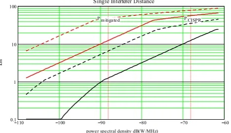
Fig. 9. Single interferer separation distances calculated forf = 1.41 GHz using the propagation model of ITU-R P.452 for flat ter-rain, but including the effects of ground clutter and curvature of the earth. Black solid line: narrow band emission at a height of 1 m, black dashed line: broad band emission. Red solid line: narrow band emission at a height of 100 m. Red dashed line: broad band emission at a height of 100 m.
around the receiver and at different heights if so required for a realistic modelling of the deployment scenario. Their aver-age distribution is set to match the averaver-age deployment val-ues and emission levels. One then calculates the sum of their signal powers using known propagation mechanisms to ob-tain the received interference power for each trial. The results statistically evaluated and plotted in histograms like the one shown in Fig. 9 for the 1.4 GHz scenario outlined above. For an assumed deployment density of 1 km−2and two possible operational heights we find that the average received power level amounts to−177 dB(W), exceeding the threshold ITU-R 769 threshold of−204 dB(W) by 27 dB, the median is at
−181 dB(W) and in 2 % of all cases, the threshold was ex-ceeded by more than 36 dB.
Although transmitter emissions are not permitted in the band we have just studied, radiation by electronic devices cannot be totally avoided and, an aggregation study may in-dicate the probability of interference when the deployment density of devices is known and their emissions are already reduced by technical or operational means. Different inter-ference probabilities are needed depending on the allocation and protection status of the band. For shared bands (Radio Regulations FN 5.149) a 2 % interference probability is ac-cepted as a practical measure, however purely passive bands require much lower interference probabilities derivable from the threshold values and the noise statistics. In addition one has to be aware of and take precautions for the fact, that a prediction of deployment characteristics for any new device is always conjectural and the actual level of interference from widely distributed license-free devices can only be known when deployment numbers have stabilised.
1 10 21 1 10 20 1 10 19 1 10 18 1 10 17 1 10 16 0
10 20 30
40 Distribution of received RFI Power
W
N
P lim P avg
Fig. 10. Histogram of received power levels for 500 trials with
random placements of narrow band CISPR-11 certified devices at 1.4 GHz within a range of 92 km from the radio telescope. The con-tributions from two operational heights (1 m and 100 m) were aver-aged for each of the 84 placements per trial for a deployment density
of 1 km−2. Average signal values are 27 dB above the ITU-R RA
769 limits designated byPlim.
6 Conclusions
In the past, radio observatories and other passive services have had the opportunity of choosing remote, radio quiet ru-ral locations which had a significantly lower level of man-made interference. The proliferation of fast switching power equipment and other digital technologies is a necessary step in the direction of greater energy conservation and use of re-newable energy sources. This can however result in severe interference problems for passive services such as radio as-tronomy if compatibility questions not addressed at an early stage. Regulatory administrations have recognised the prob-lem for unlicensed and uncontrolled consumer communica-tions equipment, but this is not the case for industrial devices. If a radio astronomical observation is obliterated by inter-ference, the information that could be obtained is lost. It is irrelevant if the origin of rfi is from industrial or commu-nication equipment, the distinction becomes more and more artificial with the progress of digital technology and it is now time to harmonise the emission standards for both the com-munications and the industrial realm.
Acknowledgements. The author likes to thank Mike Willis for the
use of his pathprofile program and Alex Kraus, Benjamin Winkel, Harry Smith and Reinhard Keller for support and discussions.
References
Cane, H. V.: MNRAS, 189, 465, 1979.
CISPR Guide, IEC, Geneva, available at: http://www.iec.ch/emc/ iec emc/iec emc players cispr.htm, 2010.
CRAF Newsletter 25, 7, available at: http://www.craf.eu/nwsl25. pdf, 2012.