An iterative method for common solutions of equilibrium problems and hierarchical fixed point problems

(1)

R E S E A R C H A R T I C L E

Open Access

An iterative method for common solutions of

equilibrium problems and hierarchical ﬁxed

point problems

Abdellah Bnouhachem

1,2†

_{, Suliman Al-Homidan}

3†

_{and Qamrul Hasan Ansari}

3,4*†

*_{Correspondence:}

[email protected]

3_{Department of Mathematics &}

Statistics, King Fahd University of Petroleum & Minerals, Dhahran, Saudi Arabia

4_{Department of Mathematics,}

Aligarh Muslim University, Aligarh, 202002, India

†_{Equal contributors}

Full list of author information is available at the end of the article

Abstract

The purpose of this paper is to investigate the problem of ﬁnding an approximate point of the common set of solutions of an equilibrium problem and a hierarchical ﬁxed point problem in the setting of real Hilbert spaces. We establish the strong convergence of the proposed method under some mild conditions. Several special cases are also discussed. Numerical examples are presented to illustrate the proposed method and convergence result. The results presented in this paper extend and improve some well-known results in the literature.

MSC: Primary 49J30; 47H09; secondary 47J20; 49J40

Keywords: equilibrium problems; variational inequalities; hierarchical ﬁxed point problems; ﬁxed point problems; projection method

1 Introduction

LetHbe a real Hilbert space whose inner product and norm are denoted by·,·and · , respectively. LetCbe a nonempty closed convex subset ofHandF:C×C→Rbe a bifunction. The equilibrium problem (in short, EP) is to ﬁndx∈Csuch that

F(x,y)≥, ∀y∈C. (.)

The solution set of EP (.) is denoted byEP(F).

The equilibrium problem provides a uniﬁed, natural, innovative and general framework to study a wide class of problems arising in ﬁnance, economics, network analysis, trans-portation, elasticity and optimization. The theory of equilibrium problems has witnessed an explosive growth in theoretical advances and applications across all disciplines of pure and applied sciences; see [–] and the references therein.

IfF(x,y) =Ax,y–x, whereA:C→His a nonlinear operator, then EP (.) is equiva-lent to ﬁnd a vectorx∈Csuch that

y–x,Ax ≥, ∀y∈C. (.)

It is a well-known classical variational inequality problem. We now have a variety of tech-niques to suggest and analyze various iterative algorithms for solving variational inequal-ities and the related optimization problems; see [–] and the references therein.

(2)

The ﬁxed point problem for the mappingT:C→His to ﬁndx∈Csuch that

Tx=x. (.)

We denote byF(T) the set of solutions of (.). It is well known thatF(T) is closed and convex, andPF(T) is well deﬁned.

LetS:C→Hbe a nonexpansive mapping, that is,Sx–Sy ≤ x–yfor allx,y∈C. The hierarchical ﬁxed point problem (in short, HFPP) is to ﬁndx∈F(T) such that

x–Sx,y–x ≥, ∀y∈F(T). (.)

It is linked with some monotone variational inequalities and convex programming prob-lems; see []. Various methods have been proposed to solve HFPP (.); see, for example, [–] and the references therein. In , Yaoet al.[] studied the following iterative algorithm to solve HFPP (.):

yn=βnSxn+ ( –βn)xn, xn+=PC

αnf(xn) + ( –αn)Tyn

, ∀n≥,

(.)

wheref:C→His a contraction mapping and{αn}and{βn}are sequences in (, ).

Un-der certain restrictions on the parameters, They proved that the sequence{xn}generated

by (.) converges strongly toz∈F(T), which is also a unique solution of the following variational inequality:

(I–f)z,y–z≥, ∀y∈F(T). (.)

In , Cenget al.[] investigated the following iterative method:

xn+=PC

αnρU(xn) + (I–αnμF)

T(yn)

, ∀n≥, (.)

whereUis a Lipschitzian mapping, andFis a Lipschitzian and strongly monotone map-ping. They proved that under some approximate assumptions on the operators and pa-rameters, the sequence{xn}generated by (.) converges strongly to a unique solution of

the variational inequality:

ρU(z) –μF(z),x–z≥, ∀x∈Fix(T).

(3)

2 Preliminaries

We present some deﬁnitions which will be used in the sequel.

Deﬁnition . A mappingT:C→His said to bek-Lipschitz continuous if there exists a constantk>  such that

Tx–Ty ≤kx–y, ∀x,y∈C.

• Ifk= , thenT is called nonexpansive. • Ifk∈(, ), thenTis called contraction.

Deﬁnition . A mappingT:C→His said to be

(a) monotone if

Tx–Ty,x–y ≥, ∀x,y∈C;

(b) strongly monotone if there exists anα> such that

Tx–Ty,x–y ≥αx–y, ∀x,y∈C;

(c) α-inverse strongly monotone if there exists anα> such that

Tx–Ty,x–y ≥αTx–Ty, ∀x,y∈C.

It is easy to observe that everyα-inverse strongly monotone mapping is monotone and Lipschitz continuous. Also, for every nonexpansive mappingT:H→H, we have

x–T(x)–y–T(y),T(y) –T(x)≤

T(x) –x

–T(y) –y, (.)

for all (x,y)∈H×H. Therefore, for all (x,y)∈H×Fix(T), we have

x–T(x),y–T(x)≤

T(x) –x 

. (.)

The following lemma provides some basic properties of the projection ontoC.

Lemma . Let PCdenote the projection of H onto C.Then we have the following inequal-ities:

(a) z–PC[z],PC[z] –v ≥,∀z∈H,v∈C;

(b) u–v,PC[u] –PC[v] ≥ PC[u] –PC[v],∀u,v∈H;

(c) PC[u] –PC[v] ≤ u–v,∀u,v∈H;

(d) u–PC[z]≤ z–u–z–PC[z],∀z∈H,u∈C.

Assumption .[] LetF:C×C→Rbe a bifunction satisfying the following assump-tions:

(A) F(x,x) = ,∀x∈C;

(4)

(A) For eachx,y,z∈C,limt→F(tz+ ( –t)x,y)≤F(x,y);

(A) For eachx∈C,y→F(x,y)is convex and lower semicontinuous.

Lemma .[] Let C be a nonempty closed convex subset of a real Hilbert space H and F:

C×C→Rsatisfy conditions(A)-(A).For r> and x∈H,deﬁne a mapping Tr:H→C as

Tr(x) = z∈C:F(z,y) + 

ry–z,z–x ≥,∀y∈C

.

Then the following statements hold:

(i) Tris nonempty single-valued;

(ii) Tris ﬁrmly nonexpansive,that is,

_T_r₍_x_{) –}_T_r₍_y₎

≤Tr(x) –Tr(y),x–y

, ∀x,y∈H;

(iii) F(Tr) =EP(F);

(iv) EP(F)is closed and convex.

Lemma .[] Let C be a nonempty closed convex subset of a real Hilbert space H.If T:

C→C is a nonexpansive mapping withFix(T)=∅,then the mapping I–T is demiclosed at

,that is,if{xn}is a sequence in C converges weakly to x and{(I–T)xn}converges strongly to,then(I–T)x= .

Lemma .[] Let U :C→H be aτ-Lipschitzian mapping and F:C→H be a k-Lipschitzian andη-strongly monotone mapping.Then,for≤ρτ<μη,μF–ρU is(μη–

ρτ)-strongly monotone,that is,

(μF–ρU)x– (μF–ρU)y,x–y≥(μη–ρτ)x–y, ∀x,y∈C.

Lemma .[] Letλ∈(, ),μ> ,and F:C→H be an k-Lipschitzian andη-strongly monotone operator.In association with a nonexpansive mapping T:C→C,deﬁne a map-ping Tλ_:_C_→_{H by}

Tλx=Tx–λμFT(x), ∀x∈C.

Then Tλ_{is a contraction provided}_μ_<η

k,that is, Tλ_x_–_Tλ_y_≤_{( –}_λν₎_x_–_y_, _∀_x_,_y_∈_C_,

whereν=  – –μ(η–μk_).

Lemma .[] Let C be a closed convex subset of a real Hilbert space H and{xn}be a

bounded sequence in H.Assume that

(i) the weakw-limit setww(xn)⊂C,whereww(xn) ={x:xni x}

(ii) for eachz∈C,lim_n→∞xn–zexists.

(5)

Lemma .[] Let{an}be a sequence of nonnegative real numbers such that

an+≤( –υn)an+δn,

where{υn}is a sequence in(, )andδnis a sequence such that

(i) ∞_n_=υn=∞;

(ii) lim sup_n→∞δn/υn≤or

∞

n=|δn|<∞. Thenlim_n→∞an= .

3 An iterative method and strong convergence results

In this section, we propose and analyze an iterative method for ﬁnding the common solu-tions of EP (.) and HFPP (.).

LetCbe a nonempty closed convex subset of a real Hilbert spaceH. LetF:C×C→R be a bifunction that satisfy conditions (A)-(A), and letS,T:C→Cbe nonexpansive mappings such thatF(T)∩EP(F)=∅. LetF:C→Cbe ak-Lipschitzian mapping and

η-strongly monotone, and letU:C→Cbe aτ-Lipschitzian mapping.

Algorithm . For any givenx∈C, let the iterative sequences{un}, {xn}, and{yn}be

generated by ⎧ ⎪ ⎨ ⎪ ⎩

F(un,y) +_r_ny–un,un–xn ≥, ∀y∈C; yn=βnSxn+ ( –βn)un;

xn+=PC[αnρU(xn) +γnxn+ (( –γn)I–αnμF)(T(yn))], ∀n≥.

(.)

Suppose that the parameters satisfy  < μ < η_k and  ≤ ρτ < ν, where ν =  –

 –μ(η–μk_{). Also,}_{_γ

n},{αn},{βn}, and{rn}are sequences in (, ) satisfying the

fol-lowing conditions:

(a) limn→∞γn= ,γn+αn< ,

(b) limn→∞αn= and

∞

n=αn=∞,

(c) lim_n→∞(βn/αn) = ,

(d) ∞_n_=|αn––αn|<∞,

∞

n=|γn––γn|<∞and

∞

n=|βn––βn|<∞,

(e) lim inf_n→∞rn> and

_∞

n=|rn––rn|<∞.

Remark . Algorithm . can be viewed as an extension and improvement for some well-known methods.

• Ifγn= , then the proposed method is an extension and improvement of a method

studied in [, ].

• IfU=f,F=I,ρ=μ= , andγn= , then we obtain an extension and improvement of

a method considered in [].

• The contractive mappingf with a coeﬃcientα∈[, )in other papers [, , ] is extended to the cases of the Lipschitzian mappingUwith a coeﬃcient constant

γ ∈[,∞).

Lemma . Let x∗∈F(T)∩EP(F).Then{xn},{un},and{yn}are bounded.

(6)

We prove that the sequence{xn}is bounded. Without loss of generality, we can assume

thatβn≤αnfor alln≥. From (.), we have

xn+–x∗

=PC[Vn] –PC

x∗

≤αnρU(xn) +γnxn+

( –γn)I–αnμF

T(yn)

–x∗

=αn

ρU(xn) –μF

x∗+γn

xn–x∗

+( –γn)I–αnμF

T(yn)

–( –γn)I–αnμF

Tx∗

≤αnρU(xn) –μF

x∗+γnxn–x∗

+ ( –γn)×

I– αnμ  –γn

FT(yn)

–

F

Tx∗

=αnρU(xn) –ρU

x∗+ (ρU–μF)x∗+γnxn–x∗

+ ( –γn)×

FT(yn)

–

F

Tx∗

≤αnρτxn–x∗+αn(ρU–μF)x∗+γnxn–x∗

+ ( –γn)

 – αnν

 –γn

yn–x∗

=αnρτxn–x∗+αn(ρU–μF)x∗+γnxn–x∗

+ ( –γn–αnν)βnSxn+ ( –βn)un–x∗

+ ( –γn–αnν)

βnSxn–Sx∗+βnSx∗–x∗

+ ( –βn)Trn(xn) –x∗

+ ( –γn–αnν)

βnSxn–Sx∗+βnSx∗–x∗+ ( –βn)xn–x∗

+ ( –γn–αnν)

βnxn–x∗+βnSx∗–x∗+ ( –βn)xn–x∗

= –αn(ν–ρτ)xn–x∗+αn(ρU–μF)x∗

+ ( –γn–αnν)βnSx∗–x∗

≤ –αn(ν–ρτ)xn–x∗+αn(ρU–μF)x∗+βnSx∗–x∗

≤ –αn(ν–ρτ)xn–x∗+αn(ρU–μF)x∗+Sx∗–x∗

= –αn(ν–ρτ)xn–x∗+

αn(ν–ρτ)

ν–ρτ (ρU–μF)x

∗₊_Sx∗_–_x∗

≤max xn–x∗,



ν–ρτ(ρU–μF)x

(7)

where the third inequality follows from Lemma .. By induction onn, we obtain

xn–x∗≤max x–x∗, 

ν–ρτ(ρU–μF)x

∗₊_Sx∗_–_x∗_,

forn≥ andx∈C. Hence,{xn}is bounded, and consequently, we deduce that{un},{yn},

{S(xn)},{T(yn)},{F(T(yn))}, and{U(xn)}are bounded.

Lemma . Let x∗∈F(T)∩EP(F)and{xn} be a sequence generated by Algorithm.. Then the following statements hold.

(a) limn→∞xn+–xn= .

(b) The weakw-limit setww(xn) ={x:xni x} ⊂F(T).

Proof From the deﬁnition of the sequence{yn}in Algorithm ., we have

yn–yn–

≤βnSxn+ ( –βn)un–

βn–Sxn–+ ( –βn–)un– =βn(Sxn–Sxn–) + (βn–βn–)Sxn–

+ ( –βn)(un–un–) + (βn––βn)un– ≤βnxn–xn–+ ( –βn)un–un–

+|βn–βn–|

Sxn–+un–

. (.)

Sinceun=Trn(xn) andun–=Trn–(xn–), we have

F(un,y) +



rn

y–un,un–xn ≥, ∀y∈C, (.)

and

F(un–,y) + 

rn–

y–un–,un––xn– ≥, ∀y∈C. (.)

Takey=un–in (.) andy=unin (.), we get

F(un,un–) +



rn

un––un,un–xn ≥, (.)

and

F(un–,un) +



rn–

un–un–,un––xn– ≥. (.)

Adding (.) and (.), and using the monotonicity ofF, we obtain

un–un–,

un––xn–

rn–

–un–xn

rn

(8)

which implies that

≤

un–un–,

rn rn–

(un––xn–) – (un–xn)

=

un––un,un–un–+

 – rn

rn–

un––xn+ rn rn–

xn–

=

un––un,

 – rn

rn–

un––xn+

rn rn–

xn–

–un–un–

=

un––un,

 – rn

rn–

(un––xn–) + (xn––xn)

–un–un–

≤ un––un  – rn rn–

un––xn–+xn––xn

–un–un–,

and then

un––un ≤

 – rn

rn–

un––xn–+xn––xn.

Without loss of generality, assume that there exists a real numberχsuch thatrn>χ> 

for all positive integersn. Then we get

un––un ≤ xn––xn+



χ|rn––rn|un––xn–. (.)

It follows from (.) and (.) that

yn–yn–

≤βnxn–xn–+ ( –βn) xn–xn–+



χ|rn–rn–|un––xn–

+|βn–βn–|

=xn–xn–+ ( –βn)



+|βn–βn–|

. (.)

Next, we estimate that

xn+–xn=PC[Vn] –PC[Vn–]

≤αnρ

U(xn) –U(xn–)

+ (αn–αn–)ρU(xn–) +γn(xn–xn–)

+ (γn–γn–)xn– + ( –γn)×

FT(yn)

–

F

(9)

T(yn–)

–( –γn–)I–αn–μF

T(yn–)

≤αnρτxn–xn–+γnxn–xn–+ ( –γn)

 – αnν

 –γn

yn–yn–

+|γn–γn–|

xn–+T(yn–)

+|αn–αn–|ρU(xn–)+μF

T(yn–), (.)

where the second inequality follows from Lemma .. From (.) and (.), we have

xn+–xn

≤αnρτxn–xn–+γnxn–xn–

+ ( –γn–αnν) xn–xn–+



+|βn–βn–|

+|γn–γn–|

T(yn–)

≤ – (ν–ρτ)αn

xn–xn–+



+|βn–βn–|

+|γn–γn–|

T(yn–)

≤ – (ν–ρτ)αn

xn–xn–

+M



χ|rn––rn|+|βn–βn–|+|γn–γn–|+|αn–αn–|

, (.)

where

M=max

sup n≥

un––xn–,sup n≥

,sup

n≥

xn–+T(yn–),

sup n≥

ρU(xn–)+μF

T(yn–).

It follows from conditions (b), (d), (e) of Algorithm ., and Lemma . that

lim

n→∞xn+–xn= .

Next, we show thatlim_n→∞un–xn= . SinceTrnis ﬁrmly nonexpansive, we have

un–x∗ =Trn(xn) –Trn

x∗

≤un–x∗,xn–x∗

= 

un–x

∗

+xn–x∗



–un–x∗–

xn–x∗

 .

Hence, we get

un–x∗



≤xn–x∗



–un–xn

(10)

From above inequality, we have

xn+–x∗ 

=PC[Vn] –x∗,xn+–x∗

=PC[Vn] –Vn,PC[Vn] –x∗

+Vn–x∗,xn+–x∗

≤αn

ρU(xn) –μF

x∗+γn

xn–x∗

T(yn)

–( –γn)I–αnμF

Tx∗,xn+–x∗

=αnρ

U(xn) –U

x∗,xn+–x∗

+αn

ρUx∗–μFx∗,xn+–x∗

+γn

xn–x∗

,xn+–x∗

+ ( –γn)

FT(yn)

–

FTx∗,xn+–x∗

≤(αnρτ+γn)xn–x∗xn+–x∗+αn

+ ( –γn–αnν)yn–x∗xn+–x∗ ≤γn+αnρτ

 xn–x

∗

+xn+–x∗

+αn

+( –γn–αnν)  yn–x

∗

+xn+–x∗ 

≤( –αn(ν–ρτ))

 xn+–x

∗

+γn+αnρτ  xn–x

∗

+αn

+( –γn–αnν) 

βnSxn–x∗



+ ( –βn)un–x∗



≤( –αn(ν–ρτ))

 xn+–x

∗

+γn+αnρτ  xn–x

∗

+αn

+( –γn–αnν) 

βnSxn–x∗+ ( –βn)xn–x∗–un–xn

, (.)

which implies that

xn+–x∗ 

≤ γn+αnρτ

 +αn(ν–ρτ)

xn–x∗



+ αn  +αn(ν–ρτ)

+( –γn–αnν)βn  +αn(ν–ρτ)

Sxn–x∗

+( –γn–αnν)( –βn)  +αn(ν–ρτ)

xn–x∗



–un–xn

≤ γn+αnρτ

 +αn(ν–ρτ)

(11)

Sxn–x∗

+xn–x∗



–( –γn–αnν)( –βn)  +αn(ν–ρτ)

un–xn.

Hence,

( –γn–αnν)( –βn)

 +αn(ν–ρτ)

un–xn

≤ γn+αnρτ

 +αn(ν–ρτ)

xn–x∗

Sxn–x∗



+xn–x∗



–xn+–x∗ 

≤ γn+αnρτ

 +αn(ν–ρτ)

xn–x∗



Sxn–x∗



+xn–x∗+xn+–x∗xn+–xn.

Sincelimn→∞xn+–xn= ,αn→,βn→, we have

lim

n→∞un–xn= . (.)

SinceT(xn)∈C, we have

xn–T(xn)

≤ xn–xn++xn+–T(xn)

=xn–xn++PC[Vn] –PC

T(xn)

≤ xn–xn++αn

ρU(xn) –μF

T(yn)

+γn

xn–T(yn)

+T(yn) –T(xn)

≤ xn–xn++αnρU(xn) –μF

T(yn)+γnxn–T(yn)+yn–xn

T(yn)+γnxn–T(yn)

+βnSxn+ ( –βn)un–xn

T(yn)+γnxn–T(yn)

(12)

Sincelim_n→∞xn+–xn= ,γn→,αn→,βn→, andρU(xn) –μF(T(yn))and

Sxn–xnare bounded, andlimn→∞un–xn= , we obtain

lim

n→∞xn–T(xn)= .

Since{xn}is bounded, without loss of generality, we can assume thatxn x∗∈C. It

fol-lows from Lemma . thatx∗∈F(T). Therefore,ww(xn)⊂F(T).

Theorem . The sequence{xn} generated by Algorithm .converges strongly to z ∈ F(T)∩EP(F),which is also a unique solution of the variational inequality:

ρU(z) –μF(z),x–z≤, ∀x∈F(T)∩EP(F). (.)

Proof From Lemma ., we havew∈F(T) since{xn}is bounded andxn w. We show

thatw∈EP(F). Sinceun=Trn(xn), we have

F(un,y) +



rn

y–un,un–xn ≥, ∀y∈C.

It follows from the monotonicity ofFthat



rn

y–un,un–xn ≥F(y,un), ∀y∈C,

and

y–unk,

unk–xnk rnk

≥F(y,unk), ∀y∈C. (.)

Sincelim_n→∞un–xn=  andxn w, it is easy to observe thatunk→w. For any  <t≤

andy∈C, letyt=ty+ ( –t)w. Then we haveyt∈C, and from (.) we obtain

≥–

yt–unk,

unk–xnk rnk

+F(yt,unk). (.)

Sinceunk →w, it follows from (.) that

≥F(yt,w). (.)

SinceFsatisﬁes (A)-(A), it follows from (.) that

 =F(yt,yt)≤tF(yt,y) + ( –t)F(yt,w)≤tF(yt,y), (.)

which implies thatF(yt,y)≥. Lettingt→+, we have

F(w,y)≥, ∀y∈C,

which implies thatw∈EP(F). Thus, we have

(13)

Observe that the constants satisfy ≤ρτ<νand

k≥η ⇐⇒ k≥η

⇐⇒  – μη+μk≥ – μη+μη

⇐⇒  –μη–μk≥_{ –}_μη ⇐⇒ μη≥ –

 –μη–μk ⇐⇒ μη≥ν,

therefore, from Lemma ., the operatorμF–ρUisμη–ρτ strongly monotone, and we get the uniqueness of the solution of variational inequality (.), and denote it by

z∈F(T)∩EP(F).

Next, we claim thatlim sup_n→∞ρU(z) –μF(z),xn–z ≤. Since{xn}is bounded, there

exists a subsequence{xnk}of{xn}such that

lim sup n→∞

ρU(z) –μF(z),xn–z

=lim sup k→∞

ρU(z) –μF(z),xnk–z

=ρU(z) –μF(z),w–z≤. Next, we show thatxn→z. We have

xn+–z

=PC[Vn] –z,xn+–z

=PC[Vn] –Vn,PC[Vn] –z

+Vn–z,xn+–z

≤

αn

ρU(xn) –μF(z)

+γn(xn–z)

+ ( –γn)

FT(yn)

–

FT(z),xn+–z

=αnρ

U(xn) –U(z)

,xn+–z

+αn

ρU(z) –μF(z),xn+–z

+γnxn–z,xn+–z + ( –γn)

FT(yn)

–

FT(z),xn+–z

≤(γn+αnρτ)xn–zxn+–z+αn

+ ( –γn–αnν)yn–zxn+–z ≤(γn+αnρτ)xn–zxn+–z+αn

+ ( –γn–αnν)

βnSxn–Sz+βnSz–z

+ ( –βn)un–z

xn+–z

= (γn+αnρτ)xn–zxn+–z+αn

+ ( –γn–αnν)

βnSxn–Sz+βnSz–z

(14)

≤(γn+αnρτ)xn–zxn+–z+αn

+ ( –γn–αnν)

βnxn–z+βnSz–z+ ( –βn)xn–z

xn+–z

= –αn(ν–ρτ)

xn–zxn+–z+αn

+ ( –γn–αnν)βnSz–zxn+–z ≤ –αn(ν–ρτ)



xn–z+xn+–z

+αn

+ ( –γn–αnν)βnSz–zxn+–z, which implies that

xn+–z

≤ –αn(ν–ρτ)

 +αn(ν–ρτ)

xn–z+

αn

 +αn(ν–ρτ)

+( –γn–αnν)βn  +αn(ν–ρτ)

Sz–zxn+–z

≤ –αn(ν–ρτ)

xn–z

+ αn(ν–ρτ)  +αn(ν–ρτ)



ν–ρτ

+( –γn–αnν)βn

αn(ν–ρτ)

Sz–zxn+–z

.

Letυn=αn(ν–ρτ) and

δn=

αn(ν–ρτ)

 +αn(ν–ρτ)



ν–ρτ

αn(ν–ρτ)

Sz–zxn+–z

.

We have∞_n_=αn=∞and

lim sup n→∞



ν–ρτ

αn(ν–ρτ)

Sz–zxn+–z

≤.

It follows that

∞

n=

υn=∞ and lim sup n→∞

δn

υn

≤.

Thus, all the conditions of Lemma . are satisﬁed. Hence, we deduce thatxn→z. This

completes the proof.

Puttingγn=  in Algorithm ., we obtain the following result, which can be viewed as

an extension and improvement of the method studied in [].

(15)

mappings such that F(T)∩EP(F)=∅.Let F :C→C be a k-Lipschitzian mapping and

η-strongly monotone,and let U:C→C be aτ-Lipschitzian mapping.For a given x∈C,

let the iterative sequences{un},{xn}and{yn}be generated by

F(un,y) +



rn

y–un,un–xn ≥, ∀y∈C;

yn=βnSxn+ ( –βn)un; xn+=PC

αnρU(xn) + (I–αnμF)

T(yn)

, ∀n≥,

where {rn},{αn} ⊂(, ), {βn} ⊂(, ). Suppose that the parameters satisfy  <μ< η_k, ≤ρτ<ν,whereν=  – –μ(η–μk_)._Also_,{_α

n},{βn},and{rn}are sequences satis-fying conditions(b)-(e)of Algorithm..Then the sequence{xn}converges strongly to some element z∈F(T)∩EP(F),which is also a unique solution of the variational inequality:

ρU(z) –μF(z),x–z≤, ∀x∈F(T)∩EP(F).

PuttingU=f,F=I,ρ=μ= , andγn= , we obtain an extension and improvement of

the method considered in [].

Corollary . Let C be a nonempty closed convex subset of a real Hilbert space H.Let F:C×C→Rbe a bifunction that satisﬁes(A)-(A)and S,T:C→C be nonexpansive

mappings such that F(T)∩EP(F)=∅.Let f :C→C be aτ-Lipschitzian mapping.For a given x∈C,let the iterative sequences{un},{xn},and{yn}be generated by

F(un,y) +



rn

y–un,un–xn ≥, ∀y∈C;

yn=βnSxn+ ( –βn)un; xn+=PC

αnf(xn) + ( –αn)T(yn)

, ∀n≥,

where{rn},{αn},{βn}are sequences in(, )which satisfy conditions(b)-(e)of Algorithm.. Then the sequence{xn}converges strongly to some element z∈F(T)∩EP(F)which is also a unique solution of the variational inequality:

f(z) –z,x–z≤, ∀x∈F(T)∩EP(F).

4 Examples

To illustrate Algorithm . and the convergence result, we consider the following exam-ples.

Example . Letαn=__n,γn=__n,βn=_n andrn=_nn_+. Then we haveαn+γn=_n< ,

lim

n→∞αn=n→∞limγn=

 n→∞lim



n= ,

and

∞

n=

αn=

 

∞

n= 

(16)

The sequences{αn}and{γn}satisfy conditions (a) and (b). Since

lim n→∞

βn

αn

= lim n→∞



n= ,

condition (c) is satisﬁed. We compute

αn––αn=

 



n– – 

n

= 

n(n– ).

It is easy to show∞_n_=|αn––αn|<∞. Similarly, we can show

∞

n=|γn––γn|<∞and

∞

n=|βn––βn|<∞. The sequences{αn},{γn}, and{βn}satisfy condition (d). We have lim inf

n→∞ rn=lim infn→∞ n n+ = ,

and

∞

n=

|rn––rn|= ∞

n=

n_n– – n

n+ 

=

∞

n= 

n(n+ )

≤

∞

n= 

n <∞.

Then the sequence{rn}satisﬁes condition (e).

Let the mappingsT,F,S,U:R→Rbe deﬁned as

T(x) =x

, ∀x∈R,

F(x) =x+ 

 , ∀x∈R,

S(x) =x

, ∀x∈R,

U(x) = x

, ∀x∈R,

and let the mappingF:R×R→Rbe deﬁned by

F(x,y) = –x+xy+ y, ∀(x,y)∈R×R.

It is easy to show that T andSare nonexpansive mappings,F is -Lipschitzian and _ -strongly monotone andUis_-Lipschitzian. It is clear that

(17)

From the deﬁnition ofF, we have

≤F(un,y) +



rn

y–un,un–xn

= –u_n+uny+ y+



rn

(y–un)(un–xn).

Then

≤rn

–u_n+uny+ y

+yun–yxn–un+unxn

= rny+ (rnun+un–xn)y– rnun–un+unxn.

LetB(y) = rny+ (rnun+un–xn)y– rnun–un+unxn. ThenB(y) is a quadratic function

ofywith coeﬃcienta= rn,b=rnun+un–xn,c= –rnun–un+unxn. We determine the

discriminantofBas follows:

=b– ac

= (rnun+un–xn)– rn

–rnun–un+unxn

=u_n+ rnun+ unrn– xnun– xnunrn+xn

= (un+ unrn)– xn(un+ unrn) +xn

= (un+ unrn–xn).

We haveB(y)≥,∀y∈R. If it has at most one solution inR, then= , and we obtain

un= xn

 + rn

. (.)

For everyn≥, from (.), we rewrite (.) as follows:

yn=_x_nn+ ( –_n)_(+xn_r_n₎;

xn+=ρ_xn_n+x_n_n+ ( –__n)y_n–μy_n+_n.

In all the tests we takeρ=_,μ=_, andN=  for Algorithm .. In this exampleη=_,

k= ,τ =_. It is easy to show that the parameters satisfy  <μ< η_k, ≤ρτ<ν, where

ν=  – –μ(η–μk_).

The values of{un},{yn}, and{xn}with diﬀerentnare reported in Tables  and . All codes

were written in Matlab.

Remark . Table  and Figure  show that the sequences{un},{yn}, and{xn}converge

to , where{}=F(T)∩EP(F).

Example . In this example we take the same mappings and parameters as in Exam-ple . exceptT andFi.

LetT: [, ]→[, ] be deﬁned by

T(x) =x+ 

(18)

Table 1 The values of{un},{yn}, and{xn}with initial valuesx1= –40 andx1= 40

x1= –40 x1= 40

un yn xn un yn xn

n= 1 –11.428571 –13.333333 –40.000000 11.428571 13.333333 40.000000

n= 2 –5.382261 –5.980290 –23.323129 5.368132 5.964591 23.261905

n= 3 –1.702305 –1.812640 –8.085951 1.691401 1.801028 8.034153

n= 4 –0.422676 –0.440288 –2.113381 0.415900 0.433229 2.079500

n= 5 –0.089920 –0.092518 –0.464586 0.085540 0.088011 0.441955

n= 6 –0.017830 –0.018208 –0.094246 0.014702 0.015013 0.077709

n= 7 –0.003964 –0.004028 –0.021308 0.001537 0.001562 0.008260

n= 8 –0.001427 –0.001445 –0.007767 –0.000562 –0.000569 –0.003058

n= 9 –0.000907 –0.000917 –0.004990 –0.000779 –0.000787 –0.004284

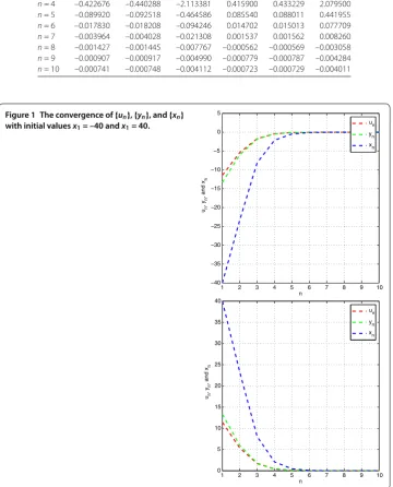
n= 10 –0.000741 –0.000748 –0.004112 –0.000723 –0.000729 –0.004011

Figure 1 The convergence of{un},{yn}, and{xn} with initial valuesx1= –40 andx1= 40.

andF: [, ]×[, ]→Rbe deﬁned by

F(x,y) = (y–x)(y+ x– ), ∀(x,y)∈[, ]×[, ].

It is clear to see that

(19)

By the deﬁnition ofF, we have

≤F(un,y) +



rn

y–un,un–xn= (y–un)(y+ un– ) +



rn

(y–un)(un–xn).

Then

≤rn(y–un)(y+ un– ) +

yun–yxn–un+unxn

=rny+ (rnun+un–xn– rn)y+ rnun–un– rnun+unxn.

LetA(y) =rny+ (rnun+un–xn– rn)y+ rnun–un– rnun+unxn. ThenA(y) is a quadratic

function ofywith coeﬃcienta=rn,b=rnun+un–xn– rn,c= rnun–un– rnun+unxn.

We determine the discriminantofAas follows:

=b– ac

= (rnun+un–xn– rn)– rn

rnun–un– rnun+unxn

= r_n– rnun– rnun+un+ rnun+ rnun+ rnxn– unxn– rnunxn+xn

= (un– rn+ unrn–xn).

We haveA(y)≥,∀y∈R. If it has at most one solution inR, then= , we obtain

un=

xn+ rn

 + rn

. (.)

For everyn≥, from (.), we rewrite (.) as follows:

yn=_x_nn+ ( –_n)(x_+n+_rr_nn);

xn+=P[,][ρ_xn_n+__nxn+ ( –__n)(yn_+)–μy_n+_n ].

(.)

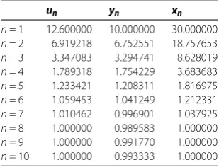
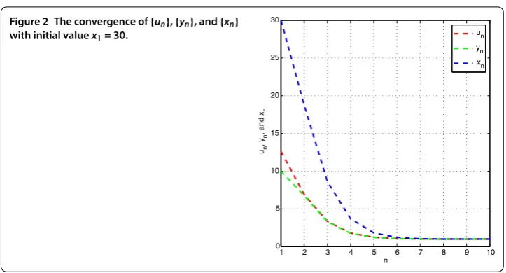
Remark . Table  and Figure  show that the sequences{un},{yn}, and{xn}converge

to , where{}=F(T)∩EP(F).

Table 2 The values of{un},{yn}, and{xn}with initial valuex1= 30

un yn xn

n= 1 12.600000 10.000000 30.000000

n= 2 6.919218 6.752551 18.757653

n= 3 3.347083 3.294741 8.628019

n= 4 1.789318 1.754229 3.683683

n= 5 1.233421 1.208311 1.816975

n= 6 1.059453 1.041249 1.212331

n= 7 1.010462 0.996901 1.037925

n= 8 1.000000 0.989583 1.000000

n= 9 1.000000 0.991770 1.000000

(20)

Figure 2 The convergence of{un},{yn}, and{xn} with initial valuex1= 30.

5 Conclusions

In this paper, we suggested and analyzed an iterative method for finding an element of the common set of solutions of (.) and (.) in real Hilbert spaces. This method can be viewed as a refinement and improvement of some existing methods for solving vari-ational inequality problem, equilibrium problem and a hierarchical fixed point problem. Some existing methods, for example, [, , , , , ], can be viewed as special cases of Algorithm .. Therefore, Algorithm . is expected to be widely applicable. In the hi-erarchical fixed point problem (.), ifS=I– (ρU–μF), then we can get the variational inequality (.). In (.), ifU=  then we get the variational inequalityF(z),x–z ≥, ∀x∈F(T)∩EP(F), which just is a variational inequality studied by Suzuki [].

Competing interests

The authors declare that they have no competing interests.

Authors’ contributions

All authors contributed equally and signiﬁcantly in writing this article. All authors read and approved the ﬁnal manuscript.

Author details

1_{School of Management Science and Engineering, Nanjing University, Nanjing, 210093, P.R. China.}2_{Ibn Zohr University,}

ENSA, BP 32/S, Agadir, Morocco.3_{Department of Mathematics & Statistics, King Fahd University of Petroleum & Minerals,}

Dhahran, Saudi Arabia.4_{Department of Mathematics, Aligarh Muslim University, Aligarh, 202002, India.}

Acknowledgements

In this research, the second and third author were ﬁnancially supported by King Fahd University of Petroleum & Minerals (KFUPM), Dhahran, Saudi Arabia. It was partially done during the visit of third author to KFUPM, Dhahran, Saudi Arabia.

Received: 30 May 2014 Accepted: 5 September 2014 Published:24 Sep 2014

References

1. Blum, E, Oettli, W: From optimization and variational inequalities to equilibrium problems. Math. Stud.63, 123-145 (1994)

2. Combettes, PL, Hirstoaga, SA: Equilibrium programming using proximal like algorithms. Math. Program.78, 29-41 (1997)

3. Combettes, PL, Hirstoaga, SA: Equilibrium programming in Hilbert space. J. Nonlinear Convex Anal.6, 117-136 (2005) 4. Ceng, LC, Yao, JC: A hybrid iterative scheme for mixed equilibrium problems and ﬁxed point problems. J. Comput.

Appl. Math.214, 186-201 (2008)

5. Takahashi, S, Takahashi, W: Strong convergence theorem for a generalized equilibrium problem and a nonexpansive mapping in a Hilbert space. Nonlinear Anal.69, 1025-1033 (2008)

6. Reich, S, Sabach, S: Three strong convergence theorems regarding iterative methods for solving equilibrium problems in reﬂexive Banach spaces. In: Optimization Theory and Related Topics. Contemp. Math., vol. 568, pp. 225-240 (2012)

(21)

8. Chang, SS, Joseph Lee, HW, Chan, CK: A new method for solving equilibrium problem ﬁxed point problem and variational inequality problem with application to optimization. Nonlinear Anal.70, 3307-3319 (2009)

9. Latif, A, Ceng, LC, Ansari, QH: Multi-step hybrid viscosity method for systems of variational inequalities defined over sets of solutions of equilibrium problem and fixed point problems. Fixed Point Theory Appl.2012, 186 (2012) 10. Marino, C, Muglia, L, Yao, Y: Viscosity methods for common solutions of equilibrium and variational inequality problems via multi-step iterative algorithms and common fixed points. Nonlinear Anal.75, 1787-1798 (2012) 11. Suwannaut, S, Kangtunyakarn, A: The combination of the set of solutions of equilibrium problem for convergence

theorem of the set of ﬁxed points of strictly pseudo-contractive mappings and variational inequalities problem. Fixed Point Theory Appl.2013, 291 (2013)

12. Yao, Y, Cho, YJ, Liou, YC: Iterative algorithms for hierarchical ﬁxed points problems and variational inequalities. Math. Comput. Model.52(9-10), 1697-1705 (2010)

13. Mainge, PE, Moudaﬁ, A: Strong convergence of an iterative method for hierarchical ﬁxed-point problems. Pac. J. Optim.3(3), 529-538 (2007)

14. Moudafi, A: Krasnoselski-Mann iteration for hierarchical fixed-point problems. Inverse Probl.23(4), 1635-1640 (2007) 15. Cianciaruso, F, Marino, G, Muglia, L, Yao, Y: On a two-steps algorithm for hierarchical fixed point problems and

variational inequalities. J. Inequal. Appl.2009, 208692 (2009)

16. Marino, G, Xu, HK: Explicit hierarchical ﬁxed point approach to variational inequalities. J. Optim. Theory Appl.149(1), 61-78 (2011)

17. Crombez, G: A hierarchical presentation of operators with ﬁxed points on Hilbert spaces. Numer. Funct. Anal. Optim. 27, 259-277 (2006)

18. Ceng, LC, Anasri, QH, Yao, JC: Some iterative methods for ﬁnding ﬁxed points and for solving constrained convex minimization problems. Nonlinear Anal.74, 5286-5302 (2011)

19. Bnouhachem, A: A modiﬁed projection method for a common solution of a system of variational inequalities, a split equilibrium problem and a hierarchical ﬁxed-point problem. Fixed Point Theory Appl.2014, 22 (2014)

20. Ceng, LC, Anasri, QH, Yao, JC: Iterative methods for triple hierarchical variational inequalities in Hilbert spaces. J. Optim. Theory Appl.151, 489-512 (2011)

21. Tian, M: A general iterative algorithm for nonexpansive mappings in Hilbert spaces. Nonlinear Anal.73, 689-694 (2010)

22. Geobel, K, Kirk, WA: Topics in Metric Fixed Point Theory. Stud. Adv. Math., vol. 28. Cambridge University Press, Cambridge (1990)

23. Suzuki, N: Moudaﬁ’s viscosity approximations with Meir-Keeler contractions. J. Math. Anal. Appl.325, 342-352 (2007) 24. Xu, HK: Iterative algorithms for nonlinear operators. J. Lond. Math. Soc.66, 240-256 (2002)

25. Acedo, GL, Xu, HK: Iterative methods for strictly pseudo-contractions in Hilbert space. Nonlinear Anal.67, 2258-2271 (2007)

26. Wang, Y, Xu, W: Strong convergence of a modiﬁed iterative algorithm for hierarchical ﬁxed point problems and variational inequalities. Fixed Point Theory Appl.2013, 121 (2013)

27. Cianciaruso, F, Marino, G, Muglia, L, Yao, Y: A hybrid projection algorithm for ﬁnding solutions of mixed equilibrium problem and variational inequality problem. Fixed Point Theory Appl.2010, 383740 (2010)

10.1186/1687-1812-2014-194