The Thirty-Third AAAI Conference on Artificial Intelligence (AAAI-19)
A Recursive Algorithm for Projected Model Counting
Jean-Marie Lagniez, Pierre Marquis
? CRIL, U. Artois & CNRSInstitut Universitaire de France? F-62300 Lens, France {lagniez, marquis}@cril.fr
Abstract
We present a recursive algorithm for projected model count-ing, i.e., the problem consisting in determining the number of modelsk∃X.Σkof a propositional formulaΣafter elim-inating from it a given setXof variables. Based on a ”stan-dard” model counter, our algorithmprojMCtakes advantage of a disjunctive decomposition scheme of∃X.Σfor comput-ingk∃X.Σk. It also looks for disjoint components in its input for improving the computation. Our experiments show that in many casesprojMCis significantly more efficient than the previous algorithms for projected model counting from the literature.
Introduction
In this paper, we are concerned with the projected model counting problem. Given a propositional formula Σand a setX of propositional variables to be forgotten, one wants to compute the number of interpretations of the variables occurring inΣbut not inX, which coincide on X with a model ofΣ. Stated otherwise, the objective is to count the number of models of the quantified Boolean formula∃X.Σ
over its variables (i.e., the variables occurring inΣbut not inX).
The projected model counting problem is a central issue to a number of AI problems (for instance, in planning, when the objective is to compute the robustness of a given plan given by the number of initial states from which the exe-cution of the plan reaches a goal state (Aziz et al. 2015)), but also outside AI (especially it proves useful in some for-mal verification problems (Klebanov, Manthey, and Muise 2013)).
Since it generalizes the standard model counting prob-lem (recovered whenX =∅), the projected model counting problem is at least as hard as the latter (#P-hard). The pres-ence of variablesXto be forgotten nevertheless may render the problem easier in some cases (thus, when every variable ofΣbelongs toX, the problem boils down to deciding the satisfiability ofΣ). That mentioned, a naive approach which would consist first in forgetting the variables ofX fromΣ, then in counting the number of models of the resulting for-mula would be impractical in many cases, in particular when
Copyright © 2019, Association for the Advancement of Artificial Intelligence (www.aaai.org). All rights reserved.
X is large. Indeed, forgetting the variables ofX fromΣin a brute-force way often leads to a formula which is much larger thanΣ(in the worst case, an exponential blow-up may occur).
Despite the importance of the problem, few algorithms for projected model counting have been pointed out so far. AnFPTalgorithm, where the parameter is the treewidth of the primal graph of the input instance, has been designed recently (Fichte et al. 2018), but this algorithm is practical only for instances having a very small treewidth. Three other algorithms for the projected model counting task have been presented in (Aziz et al. 2015), namely dSharpP,#clasp,
andd2c. Those algorithms are quite dissimilar in essence:
• dSharpP is an adaptation of the model counter dSharp
(Muise et al. 2012), which computes a Decision-DNNF representation of its inputΣto determine the number of modelskΣk.dSharpP considers as an additional input a
set P of protected variables (i.e., those variables of Σ
which should not be forgotten). The search achieved by dSharp is constrained so that the decision variables are taken in priority from P. Whenever there is no variable of P in the current formula (i.e., this formula contains only variables from X), a sat solver is used to deter-mine whether it is consistent. If so, its number of mod-els is 1, otherwise it is equal to 0. This technique has also been considered in (Klebanov, Manthey, and Muise 2013). Note that the constraint imposed on the variable or-dering limits the ability to find cutsets of small size, and this may have a strong (yet negative) impact on the quality of the conjunctive decompositions ofΣfound bydSharp.
• d2cconsists in computing first a Decision-DNNF repre-sentation ofΣ, then forgetting in it all the variables ofX (this can be achieved in linear time, but the resulting rep-resentation is not deterministic any longer in the general case). The next step consists in turning this resulting rep-resentation into aCNFone. This can be done in linear time via the introduction of new variables while preserving the number of models of the input (Tseitin 1968). Finally, the number of models of the resultingCNFformula is evalu-ated usingsharpSAT(Thurley 2006).
Unlike those algorithms, our algorithm for projected model counting, calledprojMC, is a recursive algorithm ex-ploiting a disjunctive decomposition scheme of ∃X.Σfor computingk∃X.Σk. More precisely,∃X.Σis split into an equivalent (disjunctively interpreted) set of pairwise incon-sistent formulae, so thatk∃X.Σkcan be computed by sum-ming up the corresponding projected model counts.projMC also looks for disjoint components in its input for improving the computation.
To evaluate the performance of our approach, we mea-sured the time required byprojMC for achieving the pro-jected model counting task on a number of benchmarks (uniform random3-CNFformulae, random Boolean circuits, planning instances). Our experiments show that in many casesprojMC challenges the previous algorithms for pro-jected model counting from the literature. Indeed, for some benchmarks, when compared todSharpP,#clasp, andd2c,
the time savings achieved byprojMCare of several orders of magnitude. In order to verify that the improvements ob-tained in practice withprojMCare actually due to the under-lying approach and not to the performance of the ”standard” model counter used in it (which isD4 (Lagniez and Mar-quis 2017) in our implementation), we also developedD4P,
which is the same algorithm asdSharpP, but usingD4as a
model counter instead ofdSharp. WhileD4Pperforms
typ-ically better than dSharpP (and#clasp andd2c),projMC
appears as a better performer thanD4Pfor many instances.
The rest of the paper is organized as follows. In the next section, we give some formal preliminaries. Then we describe our new projected model counter. Afterwards we present the empirical protocol which has been considered in the experiments, as well as the corresponding experi-mental results. Finally, a last section concludes the paper and gives some perspectives for further research. The binary code ofprojMC, as well as the benchmarks used in our ex-periments and additional empirical results are available from www.cril.fr/KC/.
Formal Preliminaries
LetLPbe a propositional language built up from a finite set of propositional variables P and the usual connectives.⊥ (resp.>) is the Boolean constant always false (resp. true). An interpretation (or world) ω is a mapping from P to {0,1}.The set of all interpretations is denoted W. An in-terpretation ω is a model of a formula ϕ ∈ LP if and only if it makes it true in the usual truth functional way. M od(ϕ)denotes the set of models of the formula ϕ, i.e., M od(ϕ) ={ω ∈ W |ωis a model ofϕ}.|=denotes
log-ical entailment and≡logical equivalence, i.e.,ϕ |= ψiff M od(ϕ) ⊆M od(ψ)andϕ≡ψiffM od(ϕ) = M od(ψ). Whenϕ ∈ LP andX ⊆ P,∃X.ϕis a quantified Boolean formula denoting (up to logical equivalence) the most gen-eral consequence ofϕwhich is independent from the vari-ables ofX(see e.g., (Lang, Liberatore, and Marquis 2003)).
Var(ϕ)denotes the set of variables occurring inϕ ∈ LP andVar({ϕ1, . . . , ϕk}) = S
k
i=1Var(ϕi); whenX ⊆ P, we haveVar(∃X.ϕ) =Var(ϕ)\X.
A literal` is a propositional variable or a negated one. When` is a literal overx, itscomplementary literal∼`is given by∼` = ¬xif` = xand∼` = xif ` = ¬x, and we note var(`) = x. A literal`ispurein a CNFformula
ΣwhenΣcontains no occurrence of∼`. One also says that the corresponding variablevar(`)is pure in Σ. Aterm is a conjunction of literals. It is also viewed as the set of its literals when this is convenient. Aclauseis a disjunction of literals. Whenδ=Wm
j=1`jis a clause,∼δdenotes the term given byVm
j=1∼`j. A clauseδ1is asubclauseof a clauseδ2
when every literal ofδ1is a literal ofδ2. ACNFformulaϕ
is a conjunction of clauses. It is also viewed as the set of its clauses when this is convenient.kϕkdenotes the number of models ofϕoverVar(ϕ).
Given a subsetX ofP and a worldω,ω[X]is the term
V
x∈X|ω|=xx∧
V
x∈X|ω|=¬x¬x. Theconditioningof aCNF formulaϕby a consistent termγis theCNFformulaϕ|γ obtained fromϕby removing each clause containing a lit-eral ofγand by shortening the remaining clauses, removing from them the complementary literals of those ofγ.
BCP denotes a Boolean Constraint Propagator (Zhang and Stickel 1996; Moskewicz et al. 2001), which is a key component of many solvers. BCP(Σ) returns the CNF for-mulaΣonce simplified using unit propagation.
Theprimal graphof aCNFformulaΣis the (undirected) graph where vertices correspond to the variables ofΣand an edge connecting two variables exists whenever one can find a clause ofΣwhere both variables occur. Every connected component of this graph (i.e., a maximal subset of vertices which are pairwise connected by a path) corresponds to a subset of clauses ofΣ, referred to as aconnected component of the formulaΣ.
A Recursive Algorithm
for Projected Model Counting
Our projected model counter projMC computes k∃X.Σk whereΣis aCNFformula andXa set of propositional vari-ables. AssumingΣbeing inCNFis harmless since one can use Tseitin technique (Tseitin 1968) to associate in linear time with any propositional circuit a CNF formula having the same number of models.
Unlike the previous algorithms for projected model count-ing sketched in the introductive section,projMCis a recur-sive algorithm guided by adeterministic disjunctive formfor
Σw.r.t.X. Such a form is a (disjunctively interpreted) set of formulae {ϕ1, . . . , ϕk+1} over Var(Σ) satisfying the
fol-lowing conditions:
• ∀i, j∈ {1, . . . , k+ 1}, ifi=6 jthenϕi∧ϕj|=⊥;
• Wk+1
i=1ϕi≡ >. BecauseWk+1
i=1 ϕi is valid, we have∃X.Σ ≡ (∃X.Σ)∧
(Wk+1
i=1 ϕi)≡W k+1
i=1(∃X.Σ)∧ϕi≡W k+1
i=1 ∃X.(Σ∧ϕi)since no element of a deterministic disjunctive form forΣw.r.t.X contains a variable ofX. Furthermore, since the elements of a deterministic disjunctive form forΣw.r.t.X are pairwise conflicting, we get thatk∃X.Σk =Pk+1
i=1 k(∃X.Σ)∧ϕik,
hence
k∃X.Σk=
k+1 X
i=1
k∃X.(Σ∧ϕi)k.
The set{Σ∧ϕi |i ∈ {1, . . . , k+ 1}}is referred to asthe disjunctive decompositionassociated with{ϕ1, . . . , ϕk+1}.
Technically speaking, such a notion of disjunctive decom-position can be related to several concepts considered in some previous works aboutSATor #SAT. On the one hand, it can be viewed as a specific case of the notion of set of scattered formulaefrom a formulaΣ(see (Hyv¨arinen, Junt-tila, and Niemel¨a 2006) for details), obtained by focusing on clauses/terms not containing any variable fromX. However, the objective pursued in (Hyv¨arinen, Junttila, and Niemel¨a 2006) was quite distinct from our own one (in this paper, the decomposition was used as a distribution method for SAT solving in grids). On the other hand, when it consists of con-sistent formulae, a deterministic disjunctive form forΣw.r.t. X forms a partition, just as theprimes of an X-partition ofΣ, used for generating anSDDrepresentation ofΣ(see (Darwiche 2011) for details). Nevertheless, the connection toSDDdoes not extend further: wheneverΣcontains vari-ables fromXand fromVar(Σ)\X, the disjunctive decom-position associated with a deterministic disjunctive form is not a(X,Var(Σ)\X)-decomposition ofΣ: disjunctive de-compositions do not aim to create formulae that do not share variables.
Clearly enough, generating a disjunctive decomposition {Σ∧ϕi | i ∈ {1, . . . , k+ 1}} associated with a deter-ministic disjunctive form forΣw.r.t.X is computationally useful for computingk∃X.Σk only if the formulaeΣ∧ϕi are somewhat more simple thanΣ. To ensure it and guar-antee the termination of projMC, one does not compute any deterministic disjunctive form for Σ w.r.t. X but one induced by a model ω of Σ (if there is not such model, then ∃X.Σ is inconsistent andk∃X.Σk = 0). One starts by considering the CNF formula Σ | ω[X] = Vk
i=1δi,
called the core ϕ1 of the deterministic disjunctive form
{ϕ1, . . . , ϕk+1}forΣw.r.t.X induced byω. By
construc-tion,ϕ1 =V
k
i=1δi contains variables occurring inVar(Σ) but not inX. Then we generate a (disjunctively interpreted) set ofCNFformulae{ϕ2, . . . , ϕk+1}which is equivalent to
the negation of ϕ1, by defining, for each i ∈ {1, . . . , k},
ϕi+1 = (V
i−1
j=1δj)∧∼δi. By construction,{ϕ1, . . . , ϕk+1}
satisfies the conditions of a deterministic disjunctive form forΣw.r.t.X. Note also that∃X.(Σ∧ϕ1)is equivalent to
ϕ1. Indeed,∃X.(Σ∧ϕ1)is equivalent to(∃X.Σ)∧ϕ1since
ϕ1does not contain any variable ofX. Furthermore, since
ω[X]∧Σ |= Σ, we have that∃X.(ω[X]∧Σ) |= ∃X.Σ.
But ∃X.(ω[X]∧Σ) is equivalent toΣ | ω[X], hence to ϕ1, soϕ1 |= ∃X.Σ, and as a consequence (∃X.Σ)∧ϕ1
is equivalent toϕ1. Accordingly, when computing the
num-ber of models of the disjunctive decomposition{Σ∧ϕi | i ∈ {1, . . . , k+ 1}}associated with{ϕ1, . . . , ϕk+1}, one
replacesΣ∧ϕ1byϕ1. SinceVar(ϕ1)∩X =∅, one can
take advantage of a ”standard” model counter for comput-ingkϕ1kand no recursive call ofprojMCis needed (this is
a base case for the recursion).
Our algorithmprojMC also takes advantage of any con-junctive decomposition of its inputΣinto disjoint connected components whenever such a decomposition exists. Indeed, whenever Σcan be split into two sets of clauses αandβ not sharing any variable so thatΣ ≡α∧β, then the com-putation of∃X.Σcan be achieved by computing∃X.αand ∃X.β since ∃X.Σ ≡ ∃X.(α∧β) ≡ (∃X.α)∧(∃X.β). And since ∃X.α and∃X.β do not share any variable, one can computek∃X.Σk = k∃X.αk × k∃X.βk. As it is the case for the model counting problem, taking advantage of conjunctive decompositions proves to be very useful for the efficiency purpose.
Algorithm 1:projMC(Σ,X) input : aCNFformulaΣ
input : a set of variablesX to be forgotten output: the number of models of∃X.Σover
Var(Σ)\X
1 Σ←BCP(Σ)
2 ifVar(Σ)∩X=∅then returnMC(Σ) 3 ifcache(Σ)6=nilthen returncache(Σ) 4 comps←connectedComponents(Σ) 5 if#(comps)6= 1then
6 cpt ←1
7 foreachϕ∈compsdo
8 cpt ←cpt×projMC(ϕ,X)
9 else
10 ω←sat(Σ) 11 cpt ←0 12 ifω6=∅then
13 dd ←DD(Σ, ω, X) 14 foreachϕ∈dddo
15 cpt ←cpt+projMC(ϕ,X)
×2#(Var(dd)\(Var(ϕ)∪X))
16 cache(Σ)←cpt 17 returncpt
our algorithm (no recursion takes place).
At line 3 one looks into a cache to check whether or not the current formulaΣhas already been encountered during the search. The cache, initially empty, gathers pairs consist-ing of aCNFformula and the corresponding projected model count w.r.t.X. Each timeΣhas already been cached, instead of re-computingk∃X.Σkfrom scratch, it is enough to return cache(Σ). In our implementation, the cache is residual and shared with the model counterMC.
At line 4, one partitions Σ into a set of CNF formulae that are pairwise variable-independent (i.e., two distinct el-ements of comps are built up from two disjoint sets of variables).connectedComponentsis a ”standard” procedure used in previous model counters. It is based on the search for the connected components of the primal graph ofΣand it returns a setcompsofCNFformulae composed of clauses fromΣ, so that every pair of distinct formulae fromcomps
do not share any common variable.
At line 5, one tests how many connected components have been found in Σ. If there are more than one component, then at lines 6, 7, and 8, one recursively computes the pro-jected model counts corresponding to each of them, and we store incpt the product of the corresponding counts. For efficiency reasons, in our implementation, one uses a spe-cific trick that it is not made explicit in the algorithm for the sake of readibility: systematically, one sets aside all the components forming a consistent term containing as many literals as possible. For instance, if the inputΣis equal to x1∧ ¬x2∧(x3∨x4), one sets aside the two componentsx1
and¬x2to keep only the componentx3∨x4. Indeed, for a
set of components forming a consistent term like{x1,¬x2},
the corresponding projected model count is always equal to
1(whatever the variables occurring in the term belongs toX or not). HenceprojMCreturns directly1in this case, without needing to consider the literals of the term independently in distinct recursive calls.
When only one component ofΣhas been found, at line 10, one looks for a modelω ofΣoverVar(Σ). One tests at line 12 whether such a model exists. If not (ω = ∅), then Σ is inconsistent, hence so is ∃X.Σ, and the model count is 0, the value of cpt initialized at line 11. Interest-ingly, the heuristic used by the solversattries to satisfyΣ
by assigning in priority the variables fromX. A valuable consequence of this choice is that it leads to a lazy han-dling of the clauses ofΣ which contain a literal`pure in
Σand such thatvar(`) = xwithx ∈ X. Indeed, when ` is pure inΣ,`will be set to1byωso that no clauses ofΣ
containing`will belong toΣ |ω[X]. This does not invali-date the correctness of the approach since such clauses can be removed from Σwithout changing its projected model count. Thus, while the ”standard” pure literal rule (i.e., the one consisting in removing every clause ofΣcontaining a variable which is pure in Σ) cannot be applied safely (it does not preserve the number of models of its input in the general case), its restriction where only pure literals overX are considered is correct: letα(resp.β) be the subset of the clauses ofΣcontaining`(resp. not containing`). We have ∃X.Σ ≡ ∃X.(∃{x}.(α∧β)). Since`is pure inΣ,xdoes not occur inβ. Hence∃{x}.(α∧β)≡(∃{x}.α)∧β. Now,
since every clause ofαcontains`,∃{x}.αis valid, therefore ∃X.Σ≡ ∃X.β.
At line 13, one computes the disjunctive decomposition
dd associated with the deterministic disjunctive form forΣ
w.r.t.Xinduced byω. At lines 14, and 15, one sums the pro-jected model counts for the formulae belonging todd (note that when the elementsϕofdd do not contain the same set of variables, a preliminary normalization step – multiplying each count by2to the power of the number of variables oc-curring inddbut not inϕand not inX– before summing up, is necessary). Finally, at line 16, one addsΣto the cache, as-sociated with the corresponding projected model countcpt, and at line 17, one returns the value ofcpt.
Algorithm 2:DD(Σ, ω, X)
input : aCNFformulaΣ
input : a modelωofΣoverVar(Σ)
input : a set of variablesX to be forgotten output: a setdd ofCNFformulae, the disjunctive
decomposition associated with the deterministic disjunctive form forΣw.r.t.Xinduced byω
1 {δ1, . . . , δk} ←BCP(Σ|ω[X])
2 dd ← {Vki=1δi}
3 foreachδj ∈ {δ1, . . . , δk}do
4 dd ←dd∪ {Σ∧(Vlj=1−1δl)∧∼δj}
5 returndd
Algorithm 2 provides the pseudo-code of the program which generates the disjunctive decomposition associated with the deterministic disjunctive form ofΣw.r.t.Xinduced by the modelωofΣused for guiding the search. At line 1,Σ
is first conditioned by the consistent termω[X]. This means that every clause ofΣcontaining a literal belonging toω[X]
is removed fromΣ, and in the remaining clauses, every lit-eral`overXsuch that∼`is a literal ofω[X]is removed. Fi-nally, Boolean constraint propagation is applied toΣ|ω[X]
in order to simplify it further (if possible). Clearly, no vari-able ofXoccurs in the resulting (conjunctively interpreted) set of clauses {δ1, . . . , δk}, which is the core of the deter-ministic disjunctive form forΣw.r.t.X induced byω that is computed. At line 2, we first initialize the disjunctive de-compositionddas the singleton containing the core. At lines 3 and 4, we add todd kCNFformulae since the core con-tainskclauses. At line 4, the clauses ofΣsubsumed by the clauses δl are removed (this is not detailed in the pseudo-code for the sake of readability). By construction, the for-mulae of dd are pairwise inconsistent. Furthermore, every δjof the core is a subclause of a clause ofΣsince the core is obtained by conditioningΣusing a consistent term. Accord-ingly, in our implementation, whenδjis equal to a clause of
An Example. Here is an example illustrating howprojMC works. LetΣ = (x1∨x2)∧(¬x2∨x3∨x4)∧(¬x3∨x5).
LetX={x2, x3}. The formula∃X.Σis equivalent tox1∨
x4∨x5, so thatk∃X.Σk= 7.
When run onΣandX, the first instructions ofprojMC have no effect (applyingBCPdoes not changeΣ, andΣhas a unique connected component). Suppose that the modelωof
Σsetting every variable to1has been found at line 10. Then the coreΣ|ω[X]of the deterministic disjunctive form forΣ
w.r.t.Xinduced byωwill be equal tox5. As a consequence,
the other formula belonging to the disjunctive decomposi-tion associated with this deterministic disjunctive form will beΣ∧ ¬x5.
The recursive call ofprojMC on the corex5 andX will
lead to callingMConx5as expected (since no variable of
X occurs in the core). ThenMCreturns 1, and finally the recursive call of projMC onx5 returns 1×22 = 4since
the two variablesx1,x4belong to the set of variables ofdd
but not to the set of variables of the associated core (this normalization step is achieved at line 15).
The recursive call ofprojMC onΣ∧ ¬x5 andX leads
first to simplify Σ∧ ¬x5 using BCP, so that the formula
¬x5∧(x1∨x2)∧(¬x2∨x4)∧ ¬x3is got. Since the two
components¬x5 and¬x3form together a consistent term,
only one component actually needs to be considered, namely
(x1∨x2)∧(¬x2∨x4).
So, at that step,projMCis called on(x1∨x2)∧(¬x2∨x4)
and X. Suppose again that the model ω of Σ setting ev-ery variable to 1 has been found. Then the resulting core will be equal tox4, and the resulting disjunctive
decomposi-tion will be {x4, (x1 ∨x2) ∧(¬x2∨x4)∧ ¬x4}. Since
¬x4 does not contain a variable of X, at the next
recur-sive call toprojMC,MCis used to compute its model count, equal to 1, and finally the recursive call of projMC on x4
returns1×21 = 2since the variablex
1belongs to the set
of variables of the disjunctive decomposition but not to the set of variables of the associated core. The recursive call of projMCon(x1∨x2)∧(¬x2∨x4)∧ ¬x4andXleads first to
simplify (usingBCP) the input intox1∧ ¬x2∧ ¬x4, which
is a consistent term. Hence it has only1 model. Thus one obtains thatk∃X.((x1∨x2)∧(¬x2∨x4))k= 2 + 1 = 3.
Finally the previously computed counts are summed up. One thus gets4 + 3 = 7models, as expected.
Interestingly, it can be observed thatprojMChandles ad-equately the cases when X = ∅or X = Var(Σ), in the sense that it does not waste too much time in many re-cursive calls for any of those two ”extreme” situations. In-deed, whenX =∅,projMCmainly boils down to calling a ”standard” model counterMC(line 2), as expected. When X =Var(Σ), ifΣis unsatisfiable, then it will be detected as such during the first call toprojMC(line 12) and a count of0will be returned. In the remaining case, a modelωofΣ
will be found. The core of the deterministic disjunctive form forΣw.r.t.X induced byωwill be equal to the empty set of clauses sinceΣ|ω[Var(Σ)]is valid whenωis a model ofΣ. Hence the disjunctive decomposition associated with this deterministic disjunctive form will consist only of this core. Because this core contains no variable, the next recur-sive call toprojMC(i.e., the one with the core as an operand)
will mainly consist in calling the model counterMC(line 2) on it, andMCwill return1in this case.
Finally, one can prove that our algorithmprojMCactually does the job for which it has been designed:
Proposition 1 Algorithm 1 is correct and terminates.
Proof:The correctness ofprojMC(i.e., the fact that the re-sult provided is equal tok∃X.Σkon inputsΣandX) comes from the fact that each rule used in the algorithm is sound w.r.t. the projected model counting task, as explained previ-ously. The key equalities arek∃X.Σk = Pk+1
i=1 k∃X.(Σ∧
ϕi)kfor any deterministic disjunctive form{ϕ1, . . . , ϕk+1}
for Σw.r.t. X, andk∃X.(α∧β)k = k∃X.αk × k∃X.βk whenVar(α)∩Var(β) =∅.
The termination ofprojMCcomes from the fact that each time a deterministic disjunctive form forΣw.r.t.Xis com-puted, its core does not contain any variable ofX, so that the recursive call toprojMC concerning it will lead to the base case of the recursion (line 2). As to the other disjoints
Σ∧ϕi of the corresponding disjunctive decomposition, by construction, everyϕi contains the negation of a subclause δi−1ofΣ. Hence, at the next call toprojMCconcerning this
disjoint, the literals of the term∼δi−1will be assigned and
the corresponding variables will be removed from the in-put using Boolean constraint propagation (line 1). Thus the number of variables of the input strictly diminishes at each step and this ensures the termination of the algorithm.
Note that the detection of disjoint components (lines 4 to 9 in Algorithm 1) coud be frozen inprojMCwithout ques-tioning the correctness and the termination of this algorithm (however, it has a significant impact on the efficiency of the computation on some instances). Similarly, the use of a cache has no impact on the correctness or the termination of the algorithm, so that the instructions at lines 3 and 16 could be frozen as well (but again using a cache proves to be computationally useful in many cases).
Empirical Evaluation
varying planning horizons. For each problem and value of the horizon, two variants are considered, one with the goal state fixed and one where the goal is relaxed to be any viable goal. For the first variant, the projected model count to be computed represents the number of initial states the given plan can achieve the goal from. For the second variant, it gives the number of initial states plus all goal configurations that the given plan works for.
For each instance, we measured the time (in seconds) required byprojMCto achieve the projected model count-ing job. In the experiments, the model counterMCused in projMC is the top-down compilation-based model counter D4described in (Lagniez and Marquis 2017). For the sake of comparison, we have also run the previous projected model countersdSharpP,#clasp, andd2con the same instances
(those solvers are available from people.eng.unimelb.edu. au/pstuckey/countexists) and measured the corresponding computation times. In addition, we have also compared projMCwithD4P, which is the same algorithm asdSharpP,
but using D4 as the underlying model counter instead of dSharp. All the experiments have been conducted on a clus-ter of Intel Xeon E5-2643 (3.30 GHz) quad core processors with 32 GiB RAM. The kernel used was CentOS 7, Linux version 3.10.0-514.16.1.el7.x86 64. The compiler used was gcc version 5.3.1. Hyperthreading was disabled, and no memory share between cores was allowed. A time-out of 600s and a memory-out of 7.6 GiB has been considered for each instance.
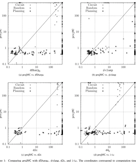
The results are reported on the scatter plots given in Fig-ure 1. Each dot represents an instance; the time (in seconds) needed to solve it using the projected model counter cor-responding to the x-axis (resp.y-axis), is given by its x -coordinate (resp.y-coordinate). Logarithmic scales are used for both coordinates. In part (a) (resp. (b), (c), (d)) of the fig-ure, thex-axis corresponds todSharpP (resp.#clasp,d2c,
D4P). They-axis corresponds toprojMCin each part of the
figure.
The four scatter plots in Figure 1 clearly show that for a great majority of instances the time needed byprojMC to count the number of projected models is smaller (and of-ten significantly smaller) than the corresponding computa-tion times when the other projected model counters are used. This is especially the case when the ”trivial” instances (i.e., those solved with a second or alike) are neglected. Notwith-standing those instances, it is interesting to observe that projMCappears at least as efficient as any of the other pro-jected model counters for all the instances from the random and the planning data sets.
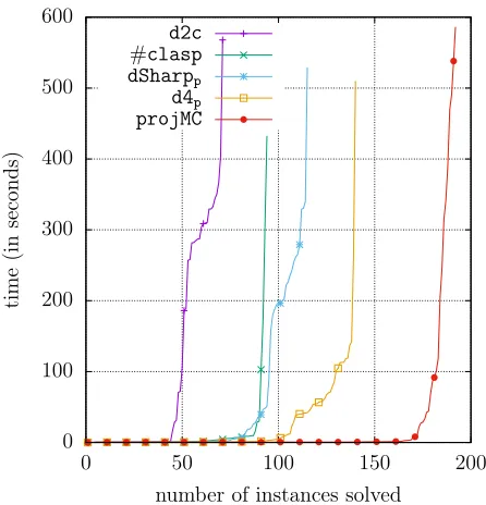
The cactus plot in Figure 2 gives fordSharpP, #clasp,
d2c,D4P, andprojMCthe number of instances solved in a
given amount of time. Clearly enough,projMCoutperforms the previous projected model counters: when the ”trivial” in-stances have been discarded,projMCtypically solves more instances than any of them in any given amount of time. Es-pecially, some significant benefits in terms of the number of instances solved have been obtained. Thus, Table 1 makes precise for each projected model counter under considera-tion the number of instances (over260) which have been solved within the time limit of 600s. It can be observed that
projMChas been able to solve many more instances than the other projected model counters.
projected model counter # of instances solved
dSharpP 115
#clasp 94
d2c 71
D4P 140
projMC 192
Table 1: Number of instances solved within the time limit depending on the projected model counter used.
Table 2 reports for each projected model counter un-der consiun-deration the number of instances which have been solved by it, and only by it.
projected model counter # of instances uniquely solved
dSharpP 0
#clasp 1
d2c 0
D4P 1
projMC 44
Table 2: Number of instances uniquely solved within the time limit depending on the projected model counter used.
Table 2 shows thatprojMCwas able to solve a significant number of instances that were out of reach for the other pro-jected model counters, given the time limit under consider-ation. That mentioned, the virtual best solver for our exper-iments would solve211 instances, which is slightly above
192. This coheres with the results reported in Figure 1 (d), showing that for the circuit instances, D4P typically
chal-lengesprojMC.
Conclusion and Perspectives
We have presented a new algorithm, projMC, for comput-ing the number of models k∃X.Σk of a propositional for-mulaΣafter eliminating from it a given setX of variables. Unlike previous algorithms, projMC takes advantage of a disjunctive decomposition scheme of ∃X.Σfor computing k∃X.Σk. It also looks for disjoint components in its in-put for improving the comin-putation. Our experiments have shown thatprojMCcan be significantly more efficient than the existing algorithms dSharpP,#clasp, and d2cfor
pro-jected model counting. Empirically,projMCalso proved bet-ter thanD4Pon many instances, showing that the improved
performance ofprojMCis not solely due to the the fact that it is ”powered” byD4.
A first perspective for further research consists in turn-ing our projected model counter into a compiler generatturn-ing
a d-DNNFrepresentation from aCNF formula containing
0.1 1 10 100
0.1 1 10 100
projMC
dSharpp Circuit
Random Planning
(a)projMCvs.dSharpP
0.1 1 10 100
0.1 1 10 100
projMC
#clasp Circuit
Random Planning
(b)projMCvs.#clasp
0.1 1 10 100
0.1 1 10 100
projMC
d2c Circuit
Random Planning
(c)projMCvs.d2c
0.1 1 10 100
0.1 1 10 100
projMC
d4p Circuit
Random Planning
(d)projMCvs.D4P
Figure 1: Comparing projMC withdSharpP,#clasp, d2c, andD4P. The coordinates correspond to computation times in
seconds. Logarithmic scales are used.
done mainly consist in modifying the instructions at lines 14 and 15 of Algorithm 1 to generate a deterministic OR node instead of making a summation. In such a compiler, when a model ofΣis generated (i.e., at a step corresponding to
0 100 200 300 400 500 600
0 50 100 150 200
time
(in
seconds)
number of instances solved d2c
#clasp dSharpp d4p projMC
Figure 2: Number of instances solved bydSharpP,#clasp,
d2c,D4P, andprojMCin a given amount of time.
elements as possible (hence a deterministic OR node with as few children as possible). In fact, one already tested this approach withinprojMC but the benefits achieved are not that significant in this case – the time spent in the maximi-sation processes can be quite large. However, things can be different when the objective is to generate a compiled rep-resentation since, in such a setting, one is typically ready to spend more off-line time in the compilation step, provided that the size of the associated compiled form is significantly smaller. We plan to make some experiments in this direction to determine whether this approach could prove useful for generating more succinct compiled representations.
A second perspective will consist in taking advantage of the two programs B and E for gate detection and re-placement within CNF formulae, used as the key compo-nents of the preprocessor for model counting reported in (Lagniez, Lonca, and Marquis 2016). Indeed,BandEcould be exploited as additional inprocessing filtering techniques inprojMC. It would be interesting to determine whether this could be computationally useful, especially for solving cir-cuit instances where, by construction, many gates can be found.
A last perspective will consist in evaluatingprojMCand the other projected model counters on other benchmarks, especially those reported in the repository available from https://github.com/dfremont/counting-benchmarks/tree/ master/benchmarks/projection.1
1
We would like to thank an anonymous reviewer for pointing out this dataset.
References
Aziz, R. A.; Chu, G.; Muise, C. J.; and Stuckey, P. J. 2015. #∃SAT: Projected model counting. InProc. of SAT’15, 121– 137.
Castell, T. 1996. Computation of prime implicates and prime implicants by a variant of the Davis and Putnam pro-cedure. InProc. of ICTAI’96, 428–429.
Darwiche, A. 2002. A compiler for deterministic decom-posable negation normal form. InAAAI’02, 627–634. Darwiche, A. 2004. New advances in compiling CNF into decomposable negation normal form. InProc. of ECAI’04, 328–332.
Darwiche, A. 2011. SDD: A new canonical representation of propositional knowledge bases. InProc. of IJCAI’11, 819– 826.
Fichte, J. K.; Hecher, M.; Morak, M.; and Woltran, S. 2018. Exploiting treewidth for projected model counting and its limits. InProc. of SAT’18, 165–184.
Gebser, M.; Kaufmann, B.; and Schaub, T. 2009. Solu-tion enumeraSolu-tion for projected Boolean search problems. In Proc. of CPAIOR’09, 71–86.
Hyv¨arinen, A. E. J.; Junttila, T. A.; and Niemel¨a, I. 2006. A distribution method for solving SAT in grids. InProc. of SAT’06, 430–435.
Klebanov, V.; Manthey, N.; and Muise, C. J. 2013. SAT-based analysis and quantification of information flow in pro-grams. InProc. of QUEST’13, 177–192.
Lagniez, J.-M., and Marquis, P. 2017. An improved decision-DNNF compiler. InProc. of IJCAI’17, 667–673. Lagniez, J.-M.; Lonca, E.; and Marquis, P. 2016. Improv-ing model countImprov-ing by leveragImprov-ing definability. InProc. of IJCAI’16, 751–757.
Lang, J.; Liberatore, P.; and Marquis, P. 2003. Propositional independence: Formula-variable independence and forget-ting.Journal of Artificial Intelligence Research18:391–443. Moskewicz, M.; Madigan, C.; Zhao, Y.; Zhang, L.; and Ma-lik, S. 2001. Chaff: Engineering an efficient SAT solver. In Proc. of DAC’01, 530–535.
Muise, C.; McIlraith, S.; Beck, J.; and Hsu, E. 2012. Dsharp: Fast d-DNNF compilation with sharpSAT. InProc. of AI’12, 356–361.
Schrag, R. 1996. Compilation for critically constrained knowledge bases. InProc. of AAAI’96, 510–515.
Thurley, M. 2006. sharpSAT - counting models with ad-vanced component caching and implicit BCP. InProc. of SAT’06, 424–429.
Tseitin, G. 1968. On the complexity of derivation in propo-sitional calculus. Steklov Mathematical Institute. chapter Structures in Constructive Mathematics and Mathematical Logic, 115–125.