THREE DIMENSIONAL PHOTOELASTIC INVESTIGATIONS
ON THICK RECTANGULAR PLATES
by
V.K. Sebastian
Civil Engineering Department University of Nigeria, Nsukka. (Manuscript received October 1980) ABSTRACT
Thick rectangular plates are investigated by means of three-dimensional photoelasticity using the stress-freezing technique. Plate with two opposite edges simply supported and the other two edges free subjected to a central line load is studied as a specific example. Three different thicknesses to include the range of thin to moderately thick to thick plates are considered and it is shown that by employing a judicious slicing pattern stress variation at the critical sections of the plate can be obtained. Numerical results obtained are compared with those from a thin plate theory and a higher order thick plate theory.
1. INTRODUCTION
It is well known that the photo-elastic method is a powerful experimental tool since it is possible by this method to obtain a complete stress field even for problems with irregular boundaries. A variety of two-dimensional problems has been solved using this technique. However, in practice many stress analysis problems exist which are strictly three-dimensional in character and cannot be effectively approached by employing two dimensional photo-elastic techniques. In recent years many
investigatorsl-6 have turned their attention to three-dimensional
photoelasticity and consequently many methods and materials are available now. However, applications to only few problems exist. Hence the present investigation aims mainly at illustrating the applicability of this method to thick plates. Square plate models of three different thicknesses were cast, machined to final dimensions and stress-frozen. In the example considered, the two opposite edges of the plate are simply supported and the remaining edges are free, the plate being subjected to a central band load. The stress-frozen model is then sliced to remove planes of interest which are then analysed to obtain stress distribution at critical sections. The results obtained from this are compared with those from Reissner and a higher order theory7.
2. MODEL PREPARATION
Models were cast in galvanised iron moulds. Galvanised iron has been found particularly suited for moulds as castings made in these moulds showed negligible initial stresses due to shrinkage compared to those made out of steel or aluminium mouIds8. The materials used are a resin, Araldite CY230, 100 parts by weight and a hardner, pthalic anhlydride, 30 parts by weight. These materials have been used by many investigators and have been found to be ideal for large casting8, 9.
The resin is first heated to a temperature of about 1100C and has been kept stirring during heating using a mechanical stirrer. The hardner, which is in the form of white flakes is slowly added to the heated resin and the mixture thoroughly mixed, the temperature always being kept between l000C and 1100C. The resin hardner mixture is properly filtered and transferred into moulds which were priorly coated with a releasing agent and kept at about 950C in a temperature controlled oven. The temperature is kept constant at 900C for about 24 hours during which the resin sets and reaches a rubbery state. It is then slowly cooled at the rate of l0C/hour to room temperature. The moulds are then stripped off and the observed in the polariscope for any possible shrinkage stresses. The models at this ,stage are usually soft and are then subjected to curing cycles by slowly heating up to 1100C and cooling as above. After the models have been significantly hardened they are machined to the required dimensions and stress frozen.
Table 1 gives the model dimensions used and the load applied. Table 1. Model dimensions and load applied
Model Dimensions in mm Concentrated load
applied in N
Model 2a =2b 2h 2c a/h
1 200 22.2 25 9 69.22
2 200 33.3 25 6 140.43
3 200 67.0 25 3 229.50
3. STRESS-FREEZING AND CALIBRATION
The model is set up inside the temperature controllable oven. The load is applied by a lever arrangement, top lever ratio of the loading frame used being four. The concentrated load coming from the loading frame will be distributed uniformly over a central band of 25 mm wide. Suitable packing of cork sheet has been placed between the model and the loading block to give a uniform loading. The loading arrangement is schematically shown in fig.1.
The model is heated relatively rapidly to about 1200C and the required load is applied. The temperature is kept fairly constant for about four hours to make it uniform throughout the model. The model is then cooled very slowly at a rate of
2 10
per hour upto about 750C and then at 10 per hour to room temperature. The model is removed and sliced for further analysis.
A circular ring and disc made out of the same material as the model and loaded along the diametral plane has also been placed in the oven along with the model to undergo the same cycle of heating and cooling. Values of E and of the material and material fringe value f are then calculated from the data obtained from the ring and the disc using the method suggested, by Durelli and FerrerlO. The calculated f, E and values for the three model are given in table 2.
4. ANALYSIS
Table 2. Material fringe value (f), modulus of elasticity (E) and Poisson’s ratio ()
f E
Model Pa-m psi-in KPa Psi at 1200C
1 332.65 1.90 12479.95 1810 0.45
2 346.66 1.98 13472.83 1954 0.46
3 336.15 1.92 13721.85 1990 0.45
is observed in a polariscope, the resulting fringe pattern cannot, in general be interpreted. The conditioned light passing through the thickness of the model integrates the secondary principal stress difference (1 - 2) over the length of the path of the light so that little can be concluded regarding the state of stress at any point.
To circumvent this difficulty the three-dimensional model is sliced to remove planes of interest which are then examined individually to determine the state of stress existing in that particular plane or slice. In studies of this type the slices should be sufficiently thin in relation to the size of the model so that stresses do not change either in magnitude or direction through the thickness of the slice. A slice
thickness of 6. 3mm
4 " 1
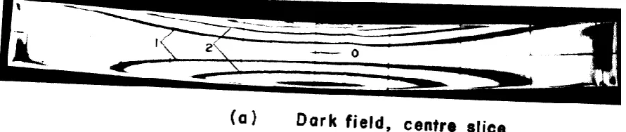
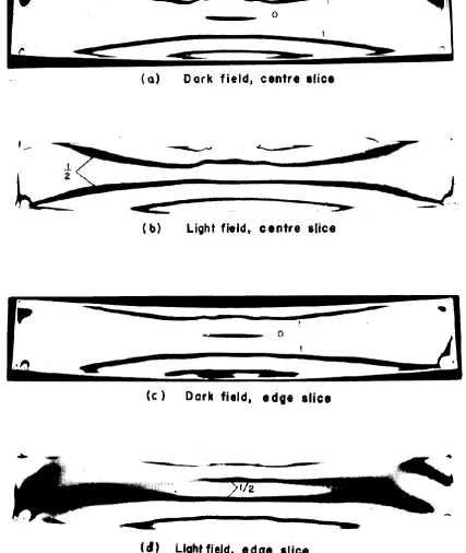
As whole field analysis is not intended only three slices, one along the x-axis called centre slice, a second at the free edge called edge slice (parallel to the x-axis) and a third one at the middle (parallel to the Y-axis) called transverse slice, as shown in fig.2, have been used. Stresses at critical points on the plate are calculated from the data obtained from these slices as follows. Some typical dark and light field isochromatic patterns obtained are shown in fig 3.
It is well-known that when a two-dimensional model is examined in a polariscope the resulting isochromatic fringe pattern can be interpreted to give9
1 - 2 = N f/t ……… (1)
Where 1 - 2 are principal stresses in the plane of the model, N is the fringe order and t is the thickness of the model.
Thus considering the centre slice which is in the xz plane, the resulting fringe pattern can be interpreted to give
1 - 2 = Ny f/t ……… (2)
and because of the symmetry in location of the centre slice, equation (2) for the top and bottom layers namely z = ±h, is written as
x - z = N f/t ……… (3)
z values on z = ±h are known to be equal to the applied load if any. The
isochromatic fringe order Ny on z = ±h
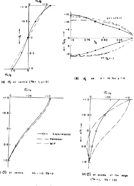
are also measured by observing the slice in the polariscope and surface values of x on z = ±h along the centre slice are then calculated using eq.(2) These variations for the three different models are shown in figs. 4(b),5(b) and 6 (b).
The x variations at the top and bottom faces of the free edge can also be determined in a similar manner.
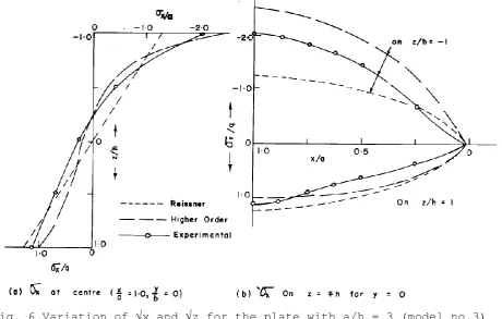
Fig. 6 Variation of x and z for the plate with a/h = 3 (model no.3)
(4)
.
...
...
o
z
δ
σz
δ
y
δ
yz
δτ
x
δ
z
x
δτ
is numerically integrated and which when written in th finite difference form is:
)
5
(
...
...
Δy
yz
Δτ
z
Δ
x
Δ
xz
Δτ
o
z
z
σ
1
z
z
σ
1 z1zo z
zo
When x = z equation (5)
) 6 ( ... ... 2 1 xz Δτ 2 1 xz Δτ o z z σ 1 z z
σ zoz zoz
By continuing this integration in a stepwise procedure it is possible to write ) 7 ( ... ... 2 xz Δτ 2 xz Δτ z z σ z z
σ 1 2 1 2
1 2 z z z z
sAnd so on whch for any z
can be written as (8) o yz Δτ )o z (σ ) z(σ
(10)
...
...
...
x
sin2θ
2t
σ
f
x
N
yz
τ
(9)
...
...
...
y
sin2θ
2t
σ
f
y
N
xz
τ
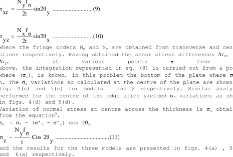
where the fringe orders Nx and Ny are obtained from transverse and centre slices respectively. Having obtained the shear stress differences xz and
yz at various points ᴥ from the
above, the integration represented in eq. (8) is carried out from a point where (z)o is known, in this problem the bottom of the plate where z = o. The z variations so calculated at the centre of the plate are shown in fig. 4(c) and 5(c) for models 1 and 2 respectively. Similar analysis performed for the centre of the edge slice yielded z variations as shown in figs. 4(d) and 5(d).
Variation of normal stress at centre across the thickness is x obtained from the equation9.
x = z – (’1 - ’2) cos 2y
(11)
...
...
...
...
y
2θ
Cos
t
σ
f
y
N
z
σ
and the results for the three models are presented in figs. 4(a) , 5(a) and 6(a) respectively.
5·NUMERICAL RESULTS AND DISCUSSION
From the dimensions of the model shown in table 1 it can be seen that the thicknesses were so chosen to include examples on a thin (a/h = 9),a moderately thick (a/h = 6) and a thick (a/h = 3) plate. It has been found that the load applied should be sufficiently large to produce enough number of fringes lest the accuracy of the results will be considerably affected. It was noticed that the load applied for models 2 and 3 should have been higher. In figs. 4 ,5 and 6 in addition to the present experimental results, those obtained from a 14th Order MIF theory 7 and Reissner or classical theory results are also shown for comparison.
In figs. 2 and 3 it can be seen that the isochromatic patterns for the centre and edge slices are nearly identical which can be expected as the plate is in cylindrical bending. The x variation predicted by experiment agrees very well with the higher order theory especially near the centre of the plate (figs. 4a, 5a and 6a). The deviation between the two near the supports (figs. 4b, 5b and 6b) may be due to the difference in edge conditions; the plate in the photoelastic experiment was supported on knife edges while In the theoretical analysis a 'friction clamped’ edge defined by boundary conditions w = x = v = o has been used. Transverse normal stress, Oz obtained from experiment compares very well with MIF theory (igs. 4c, 4d, 5c and 5d) and it can be seen that Reissner theory prediction of z at the free edge is quite different from the actual distribution but agrees very well at the centre.
6. CONCLUSION
to the conclusion that sufficiently accurate result can be obtained by this method. The experimental procedure presented will be quite useful in determination of stresses in thick plates of irregular shapes and subjected to non-typical loading for which theoretical solutions rarely exist.
ACKNOWLEDEMENT
The experimental part of the work reported in this paper was carried out by the author at the Department of Civil Engineering, Indian Institute of Science, India. The author sincerely acknowledges the help and suggestions received from Professors K. Chandrashekhara and K.T.S. Iyengar, during the course of the above investigation.
REFERENCES
1. Hetenyi, M. The fundamentals of three-dimensional photoelasticity, J. Appl. Mech., Vol. 5., 1938, pp 149-155
2 Hetenyi, M. The application of the hardening resin in three-dimensional photoelastic studies, J. Appl. Phys., Vol. 10, 1938, pp. 295-300.
3. Durelli , A.J. and R.L. Lake, Some unorthodox procedures in photoelasticity, proc, SESA, Vol. IX 1951, pp 97-122
4. Dally, J.W., A.J. Durelle and W.F. Riley, A. new method to lock-in elastic effects for experimental strees analysis, J. Appl. Mech. Vol. 25, 1958 pp. 189-195.
5. Frocht. M.N. and Pih. H., A new cornmentable material for two and three dimensional photoelastic research, Proc. SESA Vol.XII, 1954. pp 55-64.
6. Leven, M.M., Epoxy resins for photoelastic use in photoelasticity, Pergarnm press, Now York, 1963.
7. Iyengar K.T.S., Chandrashekhara, K and Sebastian, V.K., on the analysis thick rectangular plates, Igenieur - Archiv, Vol. 43, 1974, pp 317-330.
8. Chandrashekhara, K, Abraham Jacob, K, and Iyengar, K.T.S. Three-dimensional photoelastic analysis of anchorage zone stresses in post-tensioned concrete members, CBIP report, Dept. of Civil Engineering Indian I Institute of Science, Bangalore, 1974.
9. Dally, J. W. and Riley, W. F ., Experimental stress analysis McGraw-Hill Book Co., New York, 1965, pp. 252-279.