Developing an Understanding of the Steps Involved in Solving Navier—Stokes Equations »

Developing an

Understanding of the Steps

Involved in Solving Navier–

Stokes Equations

Desmond Adair

Martin Jaeger

This article describes how Mathematica can be used to develop an understanding of the basic steps involved in solving Navier– Stokes equations using a finite-volume approach for

incompressible steady-state flow. The main aim is to let students follow from a mathematical description of a given problem

through to the method of solution in a transparent way. The well-known “driven cavity” problem is used as the problem for testing the coding, and the Navier–Stokes equations are solved in vorticity-streamfunction form. Building on what the students were familiar with from a previous course, the solution algorithm for the vorticity-streamfunction equations chosen was a relaxation procedure. However, this approach converges very slowly, so another method using matrix and linear algebra concepts was also introduced to emphasize the need for efficient and

optimized code.

■

Introduction

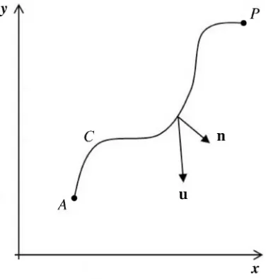
The streamfunction is defined as

ψ_A(P_{) = } A

P

u·nⅆs, (1)

where the integral has to be evaluated along a curve C from the arbitrary but fixed point A

to point P, u is the velocity vector, and n is the unit normal on the curve from A to P; see Figure 1. We regard ψA(P) as a function of the location of point P.

▲ Figure 1. Sketch illustrating the definitions of a streamfunction.

Figure 1 shows that u·n is equal to the component of the velocity u that crosses C. Therefore ψA(P) represents the volume flux (per unit depth in the z direction) through C.

Evaluating ψA(P) along two different paths and invoking the integral form of the

incom-pressibility constraint shows that ψA(P) is path independent; that is, its value only depends

on the locations of the points A and P. Changing the position of point A only changes ψA(P) by a constant. It turns out that for all applications such changes are irrelevant. It is

therefore common to suppress the explicit reference to A. Hence, we regard ψA(P) as a

function of the spatial coordinates only; that is, ψA(P) = ψ(P) = ψ(x,y). Streamlines are

lines that are everywhere tangential to the velocity field, that is, u·n, where n is the unit normal to the streamline. Hence the streamfunction ψ is constant along streamlines. Note that stationary impermeable boundaries are also characterized by u·n=0, where n is the unit normal on the boundary. Therefore, ψ is also constant along such boundaries. Invoking the integral incompressibility constraint for an infinitesimally small triangle shows that ψ is related to the two Cartesian velocity components u and v via

u= ∂ ψ

∂y; v= -−

∂ ψ

Flows that are specified by a streamfunction automatically satisfy the continuity equation, since

∂u

∂x +

∂v

∂y =

∂

∂x

∂ ψ

∂y -−

∂

∂y

∂ ψ

∂x =0. (3)

For 2D flows, the vorticity vector ω = ∇ ×u only has one nonzero component (in the z

direction); that is, ω = ωez, where

ω = ∂v ∂x -−

∂u

∂y. (4)

Using the definition of the velocities in terms of the streamfunction shows that

ω = ∂

∂x -−

∂ ψ

∂x -−

∂

∂y

∂ ψ

∂y = -− ∇

2_{ψ, (5)}

where ∇2 _{= ∂}2_{/∕ ∂x}2_{+ ∂}2_{/∕ ∂y}2 _{is the 2D Laplace operator.}

The understanding of the steps involved in solving the Navier–Stokes equations using the vorticity-streamfunction form is one of the topics used in a third-year undergraduate course on computational fluid mechanics, solely for students majoring in mechanical engi-neering. The use of Mathematica makes the assumption that the students are familiar with the package, as it generally takes a good deal of exposure to Mathematica to become com-fortable using it at the level required here [1]. The students taking the computational fluid mechanics course are indeed very familiar with Mathematica, as the computer algebra sys-tem is used during year one in the modules Calculus and Applications and Vector Calcu-lus, and during year two in the module Numerical Methods for Engineering. In addition, there are many notes, explanations, and examples on the in-house Moodle open-source learning platform. Similar work to this can be found in Fearn [2], while background read-ing on computational fluid dynamics and vorticity may be found in Ferziger and Perić [3] and Chorin [4], respectively.

■

Navier–Stokes Equations in Vorticity-Streamfunction

Form

The Navier–Stokes equations for incompressible steady-state flow in vorticity-streamfunc-tion form are

Advection-Diffusion Equation

∂ ψ

∂x

∂ ω

∂y -−

∂ ψ

∂y

∂ ω

∂x =

1

ℝe ∂2ω

∂x2 + ∂2ω

∂y2 ; (6)

Elliptic Equation

∂2_ψ

∂x2 + ∂2_ψ

∂y2 = -− ω, (7)

where ℝe is the Reynolds number. For a given problem, boundary conditions need to be specified to solve equations (6) and (7). The problem chosen here introduces the student to a classical computational fluid dynamics (CFD) case, namely the lid-driven cavity flow [5]. This flow is commonly used to test, for example, a novel method of discretization of the equations or new computer programming, as the resulting flow is well known from ex-periments. Consider a rectangular box as shown in Figure 2, where a lid is allowed to move in the horizontal plane from left to right. When the lid is not moving, the fluid in the box is stationary, whereas when the lid is moving, the fluid circulates inside the box. Here the boundary conditions needed for solution are summarized in terms of vorticity and streamfunction. As all four walls of the cavity touch, the streamfuction must be equal for all four walls, as indicated by the ψ =constant in Figure 2. The streamfuction is constant at the walls, as its gradient is velocity, which is zero relative to a given wall (no-slip tion), as indicated in the outer boxes also shown in Figure 2. The vorticity boundary condi-tions for each wall are also shown in each of these outer boxes and were derived from the streamfunction.

□

Equations in Dimensionless Form

It is convenient from a numerical point of view to make equations (6) and (7) nondimen-sional. If a and b are the height and width of the cavity, respectively, and V is a reference velocity, then

x = _bx; y= y_a; ψ = _Vbψ ; ω = ω_Vb; γ = b_a; ℝe= Vb_ν .

Equations (6) and (7) become

∂2_ω

∂x2 + γ 2 ∂

2_ω

∂y2 = ℝeγ ∂ ψ

∂y

∂ ω

∂x -−

∂ ψ

∂x

∂ ω

∂y , (8)

∂2_ψ

∂x2 + γ 2 ∂

2_ψ

∂y2 = -− ω

_{, (9)}

defined on the domain 0≤x ≤1, 0≤y ≤1. The boundary equations are defined by

ψ(x, 0) = ψ (x, 1) = ψ(0,y) = ψ (1,y) =0,

ω (x, 0) = -− γ2 ∂ 2_ψ

∂y2

y=0

,ω (x, 1) = -− γ2 ∂ 2_ψ

∂y2

y 

=1 ,

ω (0,y) = -− ∂ 2_ψ

∂x2

x 

=0

,ω (1,y) = -− ∂ 2_ψ

∂x2

x=1 .

(10)

■

Discretization and Solution Algorithm

□

Discretization of Transport Equations

▲ Figure 3. Typical Cartesian mesh used for the lid-driven cavity flow.

To discretize equations (8) and (9), the following general finite central-difference approxi-mations were introduced for spatial dimensions, obtained by adding or subtracting one Taylor series from another and invoking the intermediate value theorem. As can be seen from equation (11), the order of accuracy for both the first and second derivatives is O(h2_).

∂f(x)

∂x =

f(x+h) -−f(x-−h)

2h +Oh

2_,

∂2f(x)

∂x2 =

f(x+h) -−2f(x) +f(x-−h)

h2 +Oh

2_.

(11)

Using the approximations from equation (11), the discretized advection-diffusion equation (equation (8)) at the (i, j) node is

ω_i+1,j-−2ωij+ ωi-−1,j

h2 + γ

2 ωij+1-−2ωij+ ωij-−1

h2 =

ℝeγ ψij+1-− ψij-−1 2h

ωi,+1j-− ωi-−1,j

2h -−

ψi+1,j-− ψi-−1j

2h

ωi,j+1-− ωij-−1

2h .

(12)

The elliptic equation (equation (9)) at the (i, j) node is

ψi+1,j-−2ψij+ ψi-−1,j

h2 + γ

2 ψij+1-−2ψij+ ψij-−1

h2 = -− ω(xi,yj). (13)

□

Solution Algorithm

The solution method uses residual functions; that is, if the values of ψij and ωij are exact

on the nodes spanned by the residual functions ℛij and ℒij, then

ℛ_ijk+1= ℒ_ijk+1=0, (14)

where

ℛ_ijk+1₌ 1

2(1+ γ2₎ ψi+1,j

k _{+ ψ} i-−1,j k+1 _{+ γ}2_ψ

ij+1

k+1_{+ ψ}

ij-−1

k+1_{ +h}2_ω

ij k _{-− ψ}

ij

k_{, (15)}

ℒ_ijk+1= 1

2(1+ γ2) ωi+1,j

k _{+ ω} i-−1,j k _{+ γ}2_ω

ij+1

k _{+ ω} ij-−1

k _{ -−}ℝe

4 γψij+1

k _{-− ψ} ij-−1

k+1_{ ω}

i+1,j k _-−

ω_ik-−+1,1j -− ψik+1,j-− ψki-−+1,1j ωijk+1-− ωijk+-−11 -− ωijk.

(16)

The following fixed-point iterative procedure, based on the Gauss–Seidel scheme, is then constructed:

ψ_ijk+1_{= ℱ}k_ψ(k)_,ψ(k+1)_,ω(k)_,ω(k+1)_{ ≡ ψ} ij k_+pℛ

ij k_,

ω_ijk+1_{= 𝒢}k_ψ(k)_,ψ(k+1)_,ω(k)_,ω(k+1)_{ ≡ ω} ij k_+pℒ

ij

k_, (17)

where p is a relaxation parameter lying in the range 0<p≤1, and k+1 and k refer to the respective iterations. In this article, the actual value of p depends on ℝe and can be obtained by numerical experimentation. The use of this relaxation parameter is to improve the stability of a computation, particularly in solving steady-state problems. It works by limiting, when necessary, the amount that a variable changes from one iteration to the next. The optimum choice of p is one that is small enough to ensure stable computation but large enough to move the iterative process forward quickly.

The boundary conditions now need to be determined. For the streamfunction from equa-tion (11),

ψi,1=0 fori=1,…,nx,

ψ_nx,j=0 forj=1,…,ny,

ψi,ny =0 fori=1,…,nx, ψ1,j =0 forj=1,…,ny.

(18)

For vorticity, the following needs to be considered for, say, the left wall of the cavity with one node outside the computational domain:

ωij= -−

1

h2 ψ2,j-−2ψ1,j+ ψ0,j+ γ 2_(ψ

1,j+1-−2ψ1,j+ ψ1,j-−1). (19)

The value of ψ_0,j can be accounted for using the no-slip boundary condition on the cavity wall; that is,

v= -−∂ ψ

Using central differences, this condition can be written as

-− ∂ ψ ∂x 1,j

=0⟹ -− ψ2,j-− ψ0,j

2h =0⟹ ψ0,j= ψ2,j, (21)

where again the order of accuracy is O(h2_).

This finding, together with ψ1,j= ψ1,j+1= ψ1,j-−1=0, gives

ω1,j = -−

2

h2 (ψ2,j)forj=2,ny-−1. (22)

Similarly, for the other walls of the cavity the boundary conditions for vorticity can be deduced from

ω(xi,yi) = -−

ψi+1,j-−2ψij+ ψi-−1,j

h2 + γ

2 ψij+1-−2ψij+ ψij-−1

h2 (23)

to give

ωi,1= -− 2

h2 γ 2_(ψ

i,2)fori=1,…,nx,

ωnxj= -− 2

h2 (ψnx-−1,j)forj=2,…,ny-−1, ωiny= -−

2

h2 γ 2 _ψ

iny-−1+ h

γ i=1,…,nx,

(24)

where nx and ny are defined in Figure 3. Note that the final boundary condition shown in

equation (24) is for the moving lid, and the extra term is due to the tangential velocity being nonzero.

■

Use of

Mathematica

◼ Geometry, Mesh Parameters, Initial and Boundary Conditions

a=_{1; b}=_{1; Nx}=_{41; Ny}=_41;ℝ_e=_{100; p}=_1.0;γ =_1.;

h=a/∕ (Nx-−1) /∕/∕N;

Do[ω[i, j] =0, {i, Nx}, {j, Ny-−1}]; Do[ψ[i, j] =0, {i, Nx}, {j, Ny}];

Doω[i, Ny] = -−2γ2 ψ[i, Ny-−1] + h γ

 h2_{, {i, Nx};}

◼ Transport Equations

ℛ[i_, j_]:=

1

21+ γ2

ψ[i+1, j] + ψ[i-−1, j] + γ2(ψ[i, j-−1] + ψ[i, j+1]) +

h2ω[_{i, j}] -− ψ[_{i, j}] ℒ[i_, j_]:=

1

21+ γ2

ω[i+1, j] + ω[i-−1, j] + γ2(ω[i, j-−1] + ω[i, j+1]) -−

ℝe

4 γ ((ψ[i, j+1] -− ψ[i, j-−1]) (ω[i+1, j] -− ω[i-−1, j]) -−

(ψ[i+1, j] -− ψ[i-−1, j]) (ω[i, j+1] -− ω[i, j-−1])) -−

◼ Iterative Algorithm

With{e=0.001},

Timing

For

k=1,

Max[_Abs[_Table[ℒ[_{i, j}]_, {_{i, 2, Nx}-−₁}_, {_{j, 2, Ny}-−₁}]]] >_e,

k++, For

i=2, i<Nx, i++, For

j=2, j<Ny, j++,

ψnew[i, j] = ψ[i, j] +pℛ[i, j];

ωnew[i, j] = ω[i, j] +pℒ[i, j];

ψ[i, j] = ψnew[i, j];

ω[i, j] = ωnew[i, j];

ω[1, j] = -−2ψ[2, j] h2_;

ω[i, 1] = -−2γ2ψ[i, 2] h2;

ω[Nx, j] = -−2ψ[Nx-−1, j] h2_;

ω[i, Ny] = -−2γ2 ψ[i, Ny-−1] +h γ

 h2











◼ Streamfunction Results

ListContourPlot[

Transpose[

Partition[Flatten[Table[ψ[i, j], {i, Nx}, {j, Ny}]], Ny]], Contours→ {-−0.00005, -−0.008, -−0.1, -−0.08,-−0.05,

-−0.02, -−0.001}, ContourShading→False, AspectRatio→Automatic, ContourStyle→_Orange,

DataRange→ {{0, 1}, {0, 1}}, FrameLabel→ {x, y},

ImageSize→300,

PlotLabel→"Streamfunction Plot"

◼ Vorticity Results

ListContourPlot[

Transpose[

Partition[Flatten[Table[ω[i, j], {i, Nx}, {j, Ny}]], Ny]], Contours→ {-−5, -−3, -−1, 0, 0.25, 0.5, 0.75, 1},

ContourShading→False, ContourStyle→Orange,

DataRange→ {{0, 1}, {0, 1}}, FrameLabel→ {_{x, y}}_,

ImageSize→300,

PlotLabel→"Vorticity Plot"

]

Extraction of the centerline velocities is also instructive. First of all, students are given more experience viewing velocity profiles, and second, there are ample calculations and measurements in the literature [7, 8, 9] for comparison with the results obtained here. The centerline velocities u (in the x direction) and v (in the y direction) were derived from the streamfunction values using the equations

ui,j=

∂ ψ

∂y =

ψi,j+1-− ψi,j-−1

2h j=2,…,ny, (25)

vi,j= -−

∂ ψ

∂y =

ψi,+1j-− ψi-−1,j

The velocity distributions for u and v in the following figure are drawn along the vertical and horizontal centerlines, respectively.

Module[

{Nxm= (Nx+1) /∕2, Nym= (Ny+1) /∕2, i, j, u, v, xx}, For[j=2, j<Ny-−1, j++,

u[Nxm, j] = (ψ[Nxm, j+1] -− ψ[Nxm, j-−1]) /∕ (2 h)]; For[j=2, j<Ny-−1, j++, u[Nxm, j] = -−u[Nxm, j]]; For[_i=_{2, i}<_Nx-−_{1, i}++_,

v[i, Nym] = -− (ψ[i+1, Nym] -− ψ[i-−1, Nym]) /∕ (2 h)]; For[j=2, j<Ny-−1, j++, xx[j] = (j-−Nym) /∕Nym]; Show[

ListPlot[ {

Table[{-−u[Nxm, j], xx[j]}, {j, 2, Ny-−1}], Table[{xx[i], v[i, Nxm]}, {i, 2, Nx-−1}] },

ImageSize→_300,

AspectRatio→Automatic,

PlotLegends→ {Row[{Style["u", Italic], " m/∕s"}], Row[{Style["v", Italic], " m/∕s"}]},

PlotLabel→"CenterLine Velocities"

],

ListPlot[ {

{0.0,-−0.95}, {-−0.06, -−0.8}, {-−0.18, -−0.34},

{-−0.2, -−0.05},{-−0.2, 0.0}, {-−0.16, 0.12}, {0, 0.44},

{0.25, 0.7}, {0.5, 0.8}, {0.75, 0.9}, {0.85, 0.9} },

PlotMarkers→Graphics[{Red, Circle[]}, ImageSize→8], PlotLegends→ {"Refs. [7, 9]"}]

-−0.5 0.5

-−1.0

-−0.5 0.5

CenterLine Velocities

um/∕s

vm/∕s

Refs.[7, 9]

Importantly, the students were made aware that the profiles they calculated must be com-pared, preferably with experimental measurements, to test the validity of the calculation technique. As can be seen from the preceding figure, the calculations for the horizontal centerline velocities compare very favorably with those reported in the literature [7, 9] for ℝe=100.

■

A More Efficient and Optimized Solution Method

◼ Optimized Coding

Module[

(*⋆ global: dx, dy, sf, grid *⋆) {

ℝe=400,γ =1.,

nx=ny=N[Range[0, 50] /∕50], dh, dt=0.02,

eye, d2x, d2y,

biLeft, biRight, biBottom, biTop, bi,

vbiLeft, vbiRight, vbiBottom, vbiTop, LaplacianSV,

vort, sfSol, sfPlots

},

dh=nx[[2]] -−nx[[1]];

{eye, dx, d2x, dy, d2y} =

NDSolve`FiniteDifferenceDerivative[#, {nx, ny},

"DifferenceOrder"→₂][_{"DifferentiationMatrix"}]_&/∕@ {{0, 0}, {1, 0}, {2, 0}, {0, 1}, {0, 2}};

grid=Flatten[Outer[List, nx, ny], 1];

{biLeft, biRight, biBottom, biTop} =

Flatten[Position[grid, #]]& /∕@

{{0., y_}, {1., y_},{x_, 0.}, {x_, 1.}}; bi=DeleteDuplicates[

Flatten[{biLeft, biRight, biBottom, biTop}]];

{vbiLeft, vbiRight, vbiBottom, vbiTop} =

Flatten[_Position[_grid,#]]_& /∕@

{{dh, y_}, {1.-−dh, y_}, {x_, dh},{x_, 1.-−dh}}; LaplacianSV=eye-−dt/∕ ℝe(d2x+ γ^ 2 d2y);

LaplacianSV[[bi]] =eye[[bi]]; LUMat=LinearSolve[LaplacianSV];

vort=sf=ConstantArray[0., Length[grid]]; sfSol=Last@Reap[

Do[

rhs=vort-−dtγ (dy.sf dx.vort-−dx.sf dy.vort); rhs[[biLeft]] = -−2/∕dh ^ 2 sf[[vbiLeft]];

rhs[[biRight]] = -−2/∕dh ^ 2 sf[[vbiRight]];

rhs[[biBottom]] = -−2/∕dh ^ 2γ^ 2 sf[[vbiBottom]]; rhs[[biTop]] = -−2/∕dh ^ 2γ^ 2(sf[[vbiTop]] +dh/∕ γ); vort=LUMat[rhs];

rhs=dt/∕ ℝe vort+sf; rhs[[bi]] =0.;

sf=_LUMat[_rhs]_;

If[

Mod[timeStep-−1, 100] ⩵0,

Sow[Interpolation[Transpose[{grid, sf}]]] ],

] ];

sfPlots=Rasterize@ContourPlot[ #[x, y], {x, 0, 1}, {y, 0, 1},

Contours→ {-−_0.00005, -−_0.008, -−_0.1,-−_0.08, -−0.05,-−0.02,-−0.001, 0.001, 0.0001, 0.0005, 0.00001},

ContourShading→False, ContourStyle→Orange,

ImageSize→250]&/∕@First[sfSol];

ListAnimate[sfPlots, AnimationRunning→False] ]

U=Interpolation[Transpose[{grid, dy.sf}]]; V=Interpolation[Transpose[{grid,-−dx.sf}]];

Show[

ListLinePlot[ {

Table[{U[0.5, y], 2 y-−1}, {y, 0, 1, 1/∕100.}], Table[{2 x-−1, V[x, 0.5]}, {x, 0, 1, 1/∕100.}] }_,

PlotRange→ {{1, -−1}, {1, -−1}}, AspectRatio→1,

Axes→False, Frame→True,

PlotStyle→ {Red, Blue}, FrameStyle→Directive[Black, 12], PlotLabel→

Text[

Style[Row[{Style["U", Italic], "-−", Style["V", Italic], " Centerline Velocities"}]_{, 12}]]

],

ListPlot[

{{0.0, -−1.0}, {-−0.1, -−0.8}, {-−0.32, -−0.32},

{-−0.2, -−0.05}, {-−0.15, 0.0}, {0.0, 0.25}, {0.2, 0.5},

{0.3, 0.7}, {0.5, 0.87}, {0.75, 0.95}, {0.85, 0.97}}, PlotMarkers→Graphics[{Red, Circle[]}, ImageSize→8], PlotLegends→ {_"Refs. [_{7, 9}]_"}

] ]

Refs.[7, 9]

■

Summary

This article outlines a well-defined sequence of steps needed to solve the Navier–Stokes equations cast in the vorticity-streamfunction form. The sequence is integrated with the use of Mathematica at appropriate stages to take care of the tedious computations, and hence to allow the students to concentrate on the overall details of the solution process. In addition, it is now important to integrate computer technology so as to complete lectures and theory. This has the advantages of helping with the computations, aiding presentation for reports and analysis, and motivating students. Incorporating Mathematica also takes away the “black-box” approach so often being used by students with full CFD commercial codes, which give no real understanding of the numerics involved. The idea of efficient and optimized coding was also introduced.

■

References

[1] S. Pomeranz, “Using a Computer Algebra System to Teach the Finite Element Method,” Inter-national Journal of Engineering Education, 16(4), 2000 pp. 362–368.

www.ijee.ie/articles/Vol16-4/IJEE1162.pdf.

[2] R. L. Fearn, “Airfoil Aerodynamics Using Panel Methods,” The MathematicaJournal, 10(4), 2008 pp. 725–739.

www.mathematica-journal.com/2008/11/airfoil-aerodynamics-using-panel-methods.

[3] J. H. Ferziger and M. Perić, Computational Methods for Fluid Dynamics, 3rd ed., Berlin: Springer, 2002.

[4] A. J. Chorin, Vorticity and Turbulence (Applied Mathematical Sciences, Vol. 103), New York: Springer-Verlag, 1994.

[5] J. D. Bozeman and C. Dalton, “Numerical Study of Viscous Flow in a Cavity,” Journal of Computational Physics, 12(3), 1973 pp. 348–363. doi:10.1016/0021-9991(73)90157-5. [6] O. R. Burggraf, “Analytical and Numerical Studies of the Structure of Steady Separated

Flows,” Journal of Fluid Mechanics, 24(1), 1966 pp. 113–151. doi:10.1017/S0022112066000545.

[7] U. Gia, K. N. Ghia, and C. T. Shin, “High-Re Solutions for Incompressible Flow Using the Navier–Stokes Equations and a Multigrid Method,” Journal of Computational Physics, 48(3), 1982 pp. 387–411. doi:10.1016/0021-9991(82)90058-4.

[8] W. F. Spotz, “Accuracy and Performance of Numerical Wall Boundary Conditions for Steady, 2D, Incompressible Streamfunction Vorticity,” International Journal for Numerical Methods in Fluids, 28(4), 1998 pp. 737–757.

onlinelibrary.wiley.com/doi/10.1002/%28SICI%291097-0363%2819980930%2928:4%3C737:: AID-FLD744%3E3.0.CO;2-L/abstract.

[9] D. C. Wan, Y. C. Zhou, and G. W. Wei, “Numerical Solution of Incompressible Flows by Dis-crete Singular Convolution,” International Journal for Numerical Methods in Fluids, 38(8), 2002 pp. 789–810. doi:10.1002/fld.253.

About the Authors

Desmond Adair is a professor of mechanical engineering in the School of Engineering, Nazarbayev University, Astana, Republic of Kazakhstan. His recent research interests in-clude investigations of airborne pollution for both passive and reacting flows, and develop-ing engineerdevelop-ing mathematics by the incorporation of computer algebra systems.

Martin Jaeger is an associate professor of civil engineering and head of department in the School of Engineering, Australian College of Kuwait, Misref, Kuwait. His recent research interests include construction management and total quality, as well as developing strate-gies for engineering education.

Desmond Adair

School of Engineering Nazarbayev University 53 Kabanbay batyr Ave.

Astana, 010000, Republic of Kazakhstan [email protected]

Martin Jaeger