www.astesj.com 76
Real-Time Flux-weakening Control for an IPMSM Drive System Using a Predictive Controller
Tian-Hua Liu*, Shao-Kai Tseng, Yi Chen, Mao-Bin Lu
Department of Electrical Engineering, National Taiwan University of Science and Technology, 106, Taiwan
A R T I C L E I N F O A B S T R A C T
Received: 07 October, 2017 Accepted: 29 October, 2017 Online: 10 November, 2017
This paper proposes extended-range high-speed control for an IPMSM drive system. A simple real-time tuning flux-weakening control algorithm is proposed and implemented to control an IPMSM drive system in a wide variable speed range, from 3 r/min up to 2700 r/min. This flux-weakening control algorithm does not require any motor parameters and only needs simple mathematical computations. The proposed drive system adjusts the angle between the d-axis and q-axis current to reach flux-weakening control. In addition, a multiple sampling predictive controller is implemented to enhance the dynamic responses of the proposed drive system, which yields improved overall transient responses, superior load responses, and good tracking responses. A detailed analysis of the proposed drive system’s stability is discussed as well. A 32-bit digital signal processor, TMS-320F-28335, is used to execute the predictive controller and the flux-weakening control algorithm for the IPMSM drive system. Experimental results can validate the theoretical analysis. Keywords :
predictive controller real-time tuning flux-weakening control IPMSM
1. Introduction
Use of the interior permanent magnet synchronous motor (IPMSM) has greatly increased due to its advantages over other motors, which include high efficiency, wide operating speed range, high power density, and robustness. The IPMSM has two different torque components: electromagnetic torque and reluctance torque. By strategically controlling the d-axis and q-axis currents, the maximum torque per ampere (MTPA) control or flux weakening control can be achieved at different operating speeds.
This paper is an extension of work originally presented in 2017 IEEE 26th International Symposium on Industrial Electronics (ISIE) Conference [1]. Several researchers have proposed different flux-weakening control methods to increase the high-speed operating range of an IPMSM. For example, Bolognani et al. proposed an adaptive flux-weakening controller for an IPMSM drive system. The adaptation algorithm, however, is very complicated to implement [2]. Zhu et al. implemented a flux-weakening control for a PMSM drive system [3]. The proposed method accounted for resistance voltage drop and inverter nonlinearities. This method, however, is only suitable for a PMSM drive system, not an IPMSM drive system. Kwon et al. proposed a flux-weakening control for an IPMSM with quasi-six-step operation [4]. A feed-forward path, which consists of a one
dimensional look-up table, is required. Pan et al. proposed a robust flux-weakening control strategy for a surface-mounted permanent-magnet motor drive [5]. A closed-form solution of the maximum available torque-producing current is generated to achieve both fast responses and real-time tuning flux-weakening control. This method, however, is suitable for a surface mounted PMSM but not an IPMSM. Uddin et al. proposed an on-line parameter-estimation-based high-speed control of an IPMSM drive. The method of estimating the d-axis inductance, q-axis inductance, and external load, however, is very complicated [6]. Pan et al. proposed a voltage-constraint-based flux-weakening control of an IPMSM drive system [7]. The method requires a d-axis current command and q-axis current command generator, which is rather complicated. Jung et al. proposed a hexagonal voltage limit to increase the voltage amplitude and to improve the DC-link voltage utilization in an IPMSM drive system. A torque control method based on the voltage angle was investigated. The idea is very good; however, the voltage vector selection algorithm is very complicated [8]. Chaithongsuk et al. proposed an optimal design of permanent magnet motors to improve flux-weakening performance in variable speed drives. It was shown that a salient-pole motor performed better at high speeds than a non-salient salient-pole motor [9]. Kim proposed a novel magnetic flux-weakening method for permanent magnet synchronous motors in electric vehicles [10]. By adjusting the air gap between the stator and rotor, an increased maximum speed and maximum output power could be
ASTESJ
ISSN: 2415-6698
*Corresponding Author: Tian-Hua Liu, Mobile: +886-22737-6108
Email: [email protected]
www.astesj.com
Special issue on Advancement in Engineering Technology
obtained. This method, however, requires very complicated motor modifications. Jevremovic et al. proposed a simple robust integral controller to achieve field weakening control for a PMSM [11]. Harnefors et al. used a systematic analysis to determine the parameters of the current and speed combined controller to reduce the complicity [12]. To improve the performance of field weakening control, Wallmark et al. [13] and Bedetti et al. implemented a voltage regulator to achieve flux-weakening control for an electric vehicle and an IPMSM [14].
In this paper, a simple flux-weakening control method is proposed. This method has several advantages over previously proposed flux-weakening methods [1]-[14]. For one thing, the parameters of the IPMSM are not required. Also, the computations for the flux-weakening control are very simple. For example, only square root, multiplication, and addition are used. In addition, to achieve fast responses and good load disturbance rejection capability from the low-speed range to high-speed range, a predictive controller is employed. In contrast to previous research on predictive control [15]-[16], this paper proposes a multiple-loop predictive control motor drive system. The sampling interval of the current-loop is 100 , and the sampling interval of the speed-loop is 1 ms. Due to the quick current regulation, the proposed system has better performance than previous one-loop predictive control drive systems [15]-[16]. Unlike previous methods of flux-weakening control without using motor parameters [2], [16]-[17], the proposed method provides a simple control algorithm for voltage regulation without an adaptive controller or PI controller. To the authors’ best knowledge, the proposed flux-weakening control method is a new idea. In addition, the idea of the predictive controller applied in the simplified flux-weakening control of an IPMSM is original.
2. Predictive Controller Design
The theory of predictive control was first proposed in the 1970s, and predictive controllers have been used in chemical and steel processing for more than 40 years. Recently, predictive control has been applied in motor drives due to the fast computation ability of the digital signal processor (DSP). The design objective of a predictive controller is to compute the control input u to optimize the future dynamic behavior for the output y of the plant. This optimization must be performed within a limited time window. Several researchers have investigated predictive control for motor drives. For example, Pacas et al. proposed a predictive direct torque control for PMSMs, which yielded a faster torque settling time than the classic field-oriented control with a PI controller [15]. Bolognani et al. investigated the design and implementation of model predictive control for electric motor drives [16]. Fuentes et al. implemented a predictive speed control for a two-mass system driven by a PMSM. Their proposed method allowed feedback of all the mechanical and electrical state variables into a single control input and provided a higher bandwidth closed-loop speed control [18]. Siami et al. proposed an improved predictive current control using prediction error correction for PMSMs [19]. Tarczewski et al. implemented a constrained state feedback speed control for PMSMs, which calculated the boundaries of control signals to provide permissible values of the future state variables [20].
In this paper, a systematic predictive controller design is proposed for an IPMSM drive system. The proposed predictive controllers, including a predictive current controller and a predictive speed controller, provide a multiple sampling rate control system and a closed-loop speed-control block diagram that are different from the predictive controllers proposed in previously published papers [15]-[16], [18]-[20].
The design of a predictive controller requires the following. First, a model of the uncontrolled drive system is developed. Next, a cost function that represents the desired behavior of the system is defined. Finally, a predictive controller for the motor drive system is derived.
2.1.Predictive Current Controller
The state-variable equation of an IPMSM can be expressed as
1 1
0 0 0
1 1 ( )
0 0
0 s
d d d d d re q q
d
q q
s re d d m
q
q q
q r
L i L v L L i
i d
i v
r L i
i dt
L L
L
Where d/dt is the differential operator,
i
d and iq are the d-axis and q-d-axis stator currents,r
s is the stator resistance,v
dandq
v are the d-axis and q-axis stator voltages,
L
dandL
q are thed-axis and q-d-axis self-inductances,
m is the permanent magneticflux leakage, and
re is the electric motor speed.After transferring the continuous-time domain into the discrete-time domain, (1) can be expressed as
1
1
( ) ( )
1
cd
d d re q q
cd
z
i z v L i
z
and
1 1
( )
(
(
))
1
cq
q q re d d m
cq
z
i z
v
L i
z
The related parameters in (2) and (3) are shown as follows
s curd
r T L cd e
4a
cd 1(1 cd)
s
r
4b
s cur q
r T L cq
e
4c cq 1(1 cq)
s
r
where
T
cur is the sampling interval of current-loop control. Because the sampling time interval is shorter than the time constant of the stator current-loop, Euler approximation can be used here. As a result, the parameters shown in (4a)-(4d) can be described as follows 1 s cur
cd
d
r T
L
5a
s cur
cd d
r T
L
5b
1 s cur
cq
q
r T L
5c
and
s cur
cq q
r T
L
5d
Then (2) and (3) can be rewritten as follows
X
cur(
k
1)
A X
cur cur( )
k
B U
cur cur( )
k
B F
cur cur( )
k
6and
X
cur( )
k
i k
d( )
i k
q( )
T 7a
F
cur( )
k
re( )
k L i k
q q( )
re( )
k L i k
d d( )
m
T 7b
U
cur( )
k
v k
d( )
v k
q( )
T 7c
1 0
0 1
s cur
d cur
s cur
q r T
L A
r T L
7d
0
0 cur
d cur
cur
q T
L B
T L
7e
According to (6), the (k+1)-th predictive current can be expressed as
Xcur(k 1) A Xcur cur( )k Bcur
Ucur( )k Fcur( )k
8The performance index of the d-axis current control is defined as
* 2
(
1)
(
1)
cur d d
J
i k
i k
9The following equation is the partial differential of (9) manipulated to equal zero.
2 *
_ ( 1) ( 1)
0 ( )
d d
cur d
d d
i k i k J
U v k
10
Substituting (8) into (10), we can obtain
* 2_
(1 ) ( ) ( ) ( ) ( ) ( ) ( 1)
( ) ( )
cur s cur
d d re q q d
cur d d d
d d
T r T
i k v k k L i k i k
J L L
v k v k
*2 (1
cur s) ( ) (
cur)
( )
( )
( )
(
1)
cur0
d d re q q d
d d d
T r
T
T
i k
v k
k L i k
i k
L
L
L
11
After arranging the above, it is not difficult to obtain
(1
cur s) ( ) (
cur)
( )
( )
( )
*(
1)
d d re q q d
d d
T r
T
i k
v k
k L i k
i k
L
L
*(
d) ( )
( )
( )
( )
d(
1)
0
s d d re q q d
cur cur
L
L
r i k
v k
k L i k
i k
T
T
12
Finally, from (12), we can derive the d-axis voltage command as
*( ) ( ) d
*( 1) ( )
( ) ( )d s d d d re q q
cur
L
v k r i k i k i k k L i k
T
13
By using the same principle, we can derive the q-axis voltage command as follows
*( ) ( ) q *( 1) ( ) ( ) ( )
q s q q q re d d m
cur
L
v k r i k i k i k k L i k
T
14
2.2.Predictive Speed Controller
The differential equation of an IPMSM is
rm 1 ( e L m rm)
m
d
T T B
dt J 15
Where
J
m is the inertia,
rm is the mechanical speed,d
dt
is thedifferential operator,
T
e is the total output torque,T
L is theAccording to (15) and assuming
T
L
0
, the speed can be expressed as ( ) e
rm
m m
T s
J s B
16
By converting (16) into discrete form, one can obtain
( / ) ( / )
1 1
1
( 1) ( ) (1 ) ( )
( ) ( )
m m sp m m sp
B J T B J T
rm rm e
m
rm
k e k e T k
B
a k b u k
17
and
( / )
1
m m sp B J T
a e 18
( / )
1
1
(1 BmJmTsp)
m
b e
B
19
u k
( )
T k
e( )
20where
T
sp is the sampling interval of the speed-loop control. Next, by setting the predictive window as 1 and the predictive control as 1, the performance indexJ
sp is expressed as
1
2 *
1
1
2
1
( ) ( ) (1) ( )
( ) ( 1) pre
sp rm rm
i
i
J P z k i P k i
Q z u k i
21where
rmpre is the predictive speed,P z
( )
andQ z
( )
are polynomials ofz
, and is the weighting factor. By computing( )
sp
J
u k
, one can obtain
* 2
( ) ( 1)
2 [ ( ) ( 1)
( ) ( )
(1) ( 1)] 2 ( ) ( ) 0 pre
sp rm pre
rm
rm
J P z k
P z k
u k u k
P k Q z u k
22
Substituting (17) into (22), one can derive
*
1 1 1
2
( ) ( ) ( ) ( ) (1) ( 1)
( ) ( ) 0
rm rm
P z b P z b u k a k P k
Q z u k
23
The speed command at (k+1)th sampling interval can be expressed as a fixed command Sp and then can be defined as
*
( 1) rm k Sp
24By substituting (24) into (23), we can obtain
2 2 2
1 1 1 1
( ( ) )P z b u k( )
Q z u k( ) ( )P z b P( ) (1)SpP z b a( )
rm( )k 25
The control input can be expressed as
u k
( )
R MS
(
p
N
rm( ))
k
26and
1
(1) ( )
P M
b P z
27
1
1
a N
b
28
2 2 1
1 ( )
1 ( )
( )
R
Q z P z b
29
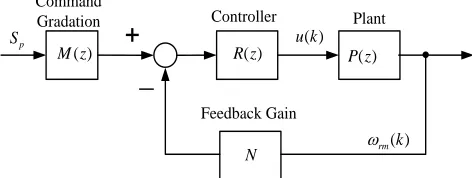
The predictive controller is shown in Figure 1. The block diagram of the predictive control includes a command gradation M(z), a controller R(z), a plant P(z), and a feedback gain N. The structure is very similar to a standard control system; however, the parameters can be systematically derived. Unlike [16], this paper outlines a systematic closed-loop block diagram of the predictive controller, which provides a clear feedback control structure for an IPMSM drive system. This is an unprecedented method of predictive control and also a major aspect of this paper.
N
( ) u k
( ) rmk ( )
R z ( )
M z p
S
+
Plant Command
Gradation Controller
Feedback Gain P(Z)
( ) P z
Figure 1 Block diagram of predictive speed-loop control.
2.3.Stability Analysis of the Proposed Drive System
The desired torque command of an IPMSM can be generated by the following equation
* 1 * *
( )
rm e L m rm
m
d
T T B
dt J 30
by the parameter variations, torque tracking errors of both MTPA and flux weakening, and external load measuring error. Then (30) can be rewritten as
* *
D
1 +
m
rm rm e
m m
B d
T T
dt J J
31
and
1 ( * * )
D m rm m rm L
m
d
T J B T
J dt
32
where
T
D is the total load disturbance,
J
m is the variation ofinertia, and
B
m is the variation of the viscous coefficient. Next, the dynamic speed equation of the IPMSM is m 1
rm rm e D
m m
B d
T T
dt J J
33
Where TD is the estimated total load disturbance, which includes
the influence of the motor parameters’ uncertainty. The tuning step of the
adv, which is 0.18 , creates a varying torque that is lessthan 1% of the output torque
T
e. As a result, the influence of the uncertainty is bound. The speed error, which is the difference between the speed command and the real speed, can be expressed as *
rm rm
e
34Taking the differential of the speed error, one can obtain
* *
(
rm rm)
rm rmd
d
d
e
dt
dt
dt
35Subtituting (31) and (33) into (35), one can obtain
*
D
1 1
( m + ) ( m )
rm e rm e D
m m m m
B B
e T T T T
J J J J
m( * )
rm rm D
m
B
T
J
36
We can define the load estimation error as TDTDTD . Assuming the external load changes slowly when compared to the quick responses of the speed control loop, it is possible to let
0.
D
T
The differential of the estimated load, therefore, can be expressed as follows TD TD 37
Define a lyapunov function as
2 2
1
1 ( D)
V e T
k
38
where
k
1 is a weighting factor. By taking the derivative of the Lyapunov function, one can derive
1
2
2 D D
V ee T T
k
39
Substituting (36) into (39), one can obtain
1
2
2 ( m )
D D D
m
B
V e e T T T
J k
2
1
1
2 m 2 ( )
D D
m
B
e T T e
J k
40
According to (40), it is possible to choose an adaption law as follows
TD k e1 41
Substituting (41) into (40), we can obtain the differential of Lyapunov function as
2 m 2 0
m
B
V e
J
42
From (42), the differential of Lyapunov function is negative semi-definite. Then, Barbalet lemma can be applied. First, a function
y
1is set, which is equal to V. Next, by integrating the
y
1, we can obtain 0
y
1( )
d
V
(0)
V
( )
43From (43), we can conclude
lim 1( ) 0
ty t 44
According to (44), the speed error converges to zero as time approaches infinity.
3. MTPA Control and Flux-weakening Control
3.1.Basic Principle
The dynamic d-q axis voltages of an IPMSM can be expressed as
d
d s d d re q q
di
v
r i
L
L i
dt
45 q
q s q q re d d re m
di
v r i L L i
dt
46
The total output torque of an IPMSM is
q d q d m
e L L i i
P
T [ ( ) ]
2 2
3
3
2 2=
[
(
)
]
2 2
m q d q s q qP
i
L
L
I
i i
47Where
I
s is the current amplitude. Two major control algorithms can be derived from (47) and can be used to adjust the torque of an IPMSM: oriented control and MTPA control. The field-oriented control sets a fixed d-axis current and adjusts the q-axis current to obtain linear proportional torque. The MTPA control sets a variable d-axis current, which is related to the q-axis current, to obtain maximum torque/ampere. The method can generate more torque than field-oriented control. However, the method creates a nonlinear relationship between the torque and q-axis current [3], which is a disadvantage of MTPA control. While it is a fact that MTPA’s influence on torque linearity is a drawback, achieving maximum torque is a greater benefit that outweighs that disadvantage. The issue will be researched further by the authors of this paper.Taking e 0
q
T di
d
and substituting it into (47), we can obtain
3 [ ( ) ( )2 1] 0
2 2 m d q d d q q d
P
L L i L L i
i
48
From (48), the d-axis current under MTPA control can be expressed as
2
2 2
|
2( ) 4( )
m m
d MTPA q
d q d q
i i
L L L L
49
The advance angle under MTPA control is
1 |
sin d MTPA MTPA
s
i
I
50
and the current amplitude
I
s is expressed as 2 2
s d q
I
i
i
51In steady-state and neglecting the voltage drops of the resistance and inductance, it is not difficult to obtain
v
d
reL i
q q 52and
v
q
reL i
d d
re m 53The voltage amplitude is
2 2
(
)
s d q
v
v
v
54If
V
om is the maximum voltage amplitude, the voltage constraint can be shown as 2 2 2
( ) ( ) ( om)
q q d d m
re
V
L i L i
55
The maximum current amplitude
I
sm can be expressed as 2 2 2
d q sm
i i I 56
From (56), it is easy to obtain
2 2
q sm d
i I i 57
Combining (49), (54), and (57), the constraints of the IPMSM drive system can be obtained. The drive system operates under MTPA control when the motor speed is below the rated base-speed. After the drive system reaches its base speed, there are two constraints: the current constraint of the maximum amplitude,
I
sm, and the voltage constraint of the maximum voltage amplitude,om
V
. However, the om reV
is decreased as the motor speed increases,
which is shown in Figure 2. As a result, the axes of the ellipse are reduced when the motor speed increases. When
re
base, the motor operates under MTPA control, which is indicated as OCBA in Figure 2. When
base
re
c, the motor operates in region II, in which the motor can operate either under MTPA control or flux-weakening control. Ifi
d
i
d MTPA|
, MTPA control is used; onthe other hand, if
i
d
i
d MTPA|
, flux-weakening control is used.When
c
re, the motor operates in region III, in which only flux-weakening control can be used.3.2.Proposed Real-Time Flux-weakening Control
In the real world, flux-weakening control is very complicated because it requires
m,
L
d,
andL
q , which are very difficult to measure [15].To solve this difficulty, in this paper, a real-time tuning flux-weakening control is proposed. First, the voltage amplitude of the IPMSM,
v
s , which is expressed in (54) is compared to theI
II
III
Fixed Torque Curve
iq(A)
MTPA Curve Current Constraint
( Is=Ism) Voltage Constraint
(Vs=Vom)
id( A)
A 1
3
B
C
base
c
2
D
O G
H
F
J K
4
4 3 2 1
max
idC
idB idD
TC TB Speed
Regions
Figure 2 Operating regions of an IPMSM.
θ
FW(k)
θ
FW(k 1)
sgn
(v -V )
s om and
sgn (
v
s
V
om)
1 when (
v
s
V
om) 0
59aand
sgn (
v
s
V
om) 1 when (
v
s
V
om) 0
59bwhere
is the step size of the real-time tuning control. By using(58), (59a), and (59b), the
FW can be real-time tuned, as shown in Figure 3(a)(b). Finally, a block diagram of the proposed real-time tuning flux-weakening control is shown in Figure 4. First, the amplitude of the desired output voltagev
s is calculated. Next, thedesired output voltage,
v
s, is compared with the measured outputvoltage,
V
om. After that, (58) is used to compute the
FW(
k
).
Similar to previous research [2]-[5], [21], the proposed flux-weakening control method reduces the torque at high-speed operating range, and is not guaranteed the torque linearity. This is a common characteristic of flux-weakening control algorithms. However, the stability analysis of the whole drive system is discussed in the previous section of this paper.Current Constraint and Voltage Constraint
base
c
Constant Torque Par t i al
Fl ux- weakeni ng
Current Constraint
Current Constraint
Voltage Constraint
A
B C
O G
H B
C G
2 e
T
max
T
re B
T
C
T
G
T
A
H MTPA
FW
MTPA
adv
sm
I
base
2
c
q
i (A)
d
i (A)
(a) (b)
Figure 3 Operating curves and torque-speed curves of an IPMSM (a) operating curves (b) torque-speed curves.
2 2
s d q
v v v
om
V z1
s
v
d
v
q
v
( 1) FW k
2
( ) FW k
Figure 4 Block diagram of the proposed flux-weakening control.
4. Implementation
The implemented IPMSM drive system is shown in Figure 5(a) and (b). Figure 5(a) is a block diagram of the proposed IPMSM. The system consists of two main parts: the DSP system and the hardware circuit. The DSP system uses a TMS-320F-28335, which is a 32-bit, digital signal processor manufactured by Texas Instruments. The sampling interval of the current-loop control is 100s, while that of the speed-loop control is 1 ms.
Taking the MTPA operating region as an example, the controller works as follows. First, as shown in Figure 5(a) and based on the predictive speed controller, after the speed command is input and the motor speed is feedback, the q-axis current control
qp
i is computed. Second, the load compensator compensates for
the load disturbance TD and then generates the compensation
current TD q
i
. Then the total q-axis current command, which is thesummation of the iqp and TD q
i
, is computed and expressed as iq*.Next, the d-axis current is computed through (49) when the motor is operating in the MTPA region. After that, the advance phase angle
MTPA and stator current amplitudeI
s* are computed by using (50) and (51). Finally, the flux-weakening is obtained byadding
FW.By using the MTPA table and the real-time tuning flux-weakening control, the advance angle of the current can be obtained. After that, the d-axis current command id* and the q-axis current command *
q
i are calculated. A current regulated control and a space vector PWM modulation are executed. Finally, the switching states of the inverter are determined and output. A closed-loop system can thus be obtained. A DC motor is coupled with the IPMSM. The motor parameters are: Lq31 mH ,
15
d
L mH, m 0.227 .sec/v rad, and Rs1.9 . The motor is 4-pole,
1-HP, and rated at 1500 r/min.
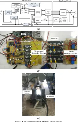
Figure 5(b) shows a photograph of the entire hardware circuit, which includes a DSP, gate drivers, peripheral devices, current sensing circuits, and an inverter. Figure 5(c) shows a photograph of the implemented IPMSM drive system, including an IPMSM and a dynamometer.
5. Experimental Results
using the MTPA control and the hybrid control, which is a combination of the MTPA control and the flux-weakening control.
Inverter IPMSM Encoder abc/dq
a
i
b
i
, ,
abc
i i i
d
i
q
i
* d
i
* q
i
Speed Calculator
rm
Real-Time Flux-Weakening
Control
* s
I
*
d
v
* q
v
* q
v
adv
* * * *
sin cos
d s adv q s adv
i I i I
FW
MTPA
Computing current Amplitude
and Phase
rm
Load Compensator
c
i dq/αβ
& SVPWM
A/D Converter
Current Sensing Circuit
a
i
b
i
DSP System Hardware Circuit
TD
q
i
qp
i
* rm
2 P
re
re
* d
v
* rm
rm
Predictive Speed Controller
*
q
I
Eq(49)
*
dMTPA
I
Predictive Current Controller
*
q
I
(a)
(b)
(c)
Figure 5 The implemented IPMSM drive system (a) block diagram (b) hardware circuit (c) motor and dynamometer.
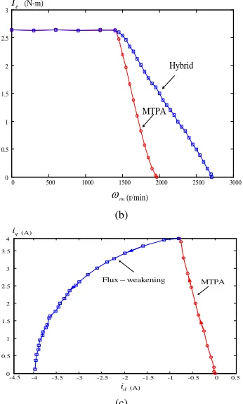
As you can observe, the hybrid control has better performance than the MTPA control. Figure 6 (c) shows the q-axis current to the d-axis current trajectory when the IPMSM is operating from the MTPA control region to the flux-weakening control region. The d-axis current increases slightly in the MTPA region; however, the d-axis current increases significantly in the flux-weakening region.
Figure 7(a)(b) and (c) show the measured waveforms of the IPMSM operating at 1800 r/min under loads of 0.57 N-m and 1.89 N-m. Figure 7(a) is the amplitude of the stator current
I
s . Figure 7(b) shows the relative measured d-axis and q-axis currents. Figure 7(c) shows the measured advance angle
adv that is the sum of theFW
and
MTPA, which are the measured flux-weakening angle and the measured MTPA control angle. The delay of the measured responses is due to the lag between the load command and the external load that is generated by the dynamometer. Figure 8(a) shows the load disturbance responses when using the proposed predictive controller, the previous predictive controller that was proposed by [21], and the PI controller. The parameters of the PIcontroller are obtained by using the pole assignment technique. The locations of the desired poles for the closed-loop drive system are assigned as -4.06+j0.13 and -4.06-j0.13, respectively. The proposed predictive controller performs better than the previous predictive controller and the PI controller. At this 2000 r/min high speed, the field weakening algorithm is applied. The maximum allowed external load at this operating speed is 1.6 N.m. Experimental results show the proposed predictive controller performs the best. Figure 8(b) shows the repetitive 1.6 N.m load disturbance responses. The proposed predictive controller performs well again.
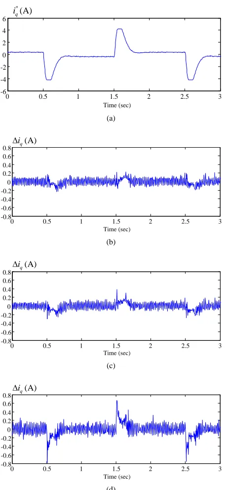
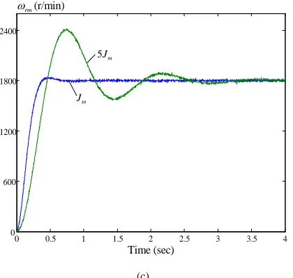
Figure 9(a) shows the measured step-input transient speed responses at the maximum speed, 2700 r/min. In this paper, the rated speed is 1500 r/min. The measured responses show the proposed predictive controller has a quicker rise time than the previous predictive controller proposed by [16] and the PI controller. Figure 9(b) shows the measured step-input transient speed responses at 3 r/min, which is the minimum operating speed. According to Figure 9(a) and Figure 9(b), we can conclude that the adjustable speed ratio of the maximum speed to minimum speed is 900:1. Figure 10 (a)(b)(c)(d) shows the current command and measured current errors using different controllers. Again, the proposed predictive controller has the smallest tracking errors. Figure 11(a)(b)(c) show the measured dynamic responses of the proposed flux-weakening control at 1800 r/min. A 5V step input at
om
V
is injected for every 1 second. The real voltage amplitude ofthe motor, which is expressed as
v
s can track the voltagecommand
V
om well. The rise time of the voltage control is about 50 ms. Figure 11(a), Figure 11(b) and Figure 11(c) show the responses of speed, voltage amplitude, and controlling angle
FW respectively. Figure 12(a) shows the measured efficiency of the whole drive system. The proposed method has higher efficiency than the linear flux-weakening method that was proposed by [21]. The major reason is that the proposed method provides greater output torque at the same motor speed. Figure 12(b) and (c) show the measured speed responses as the inertia of the drive system is increased to 5 times. The proposed predictive controller can provide a lower overshoot and a shorter settling time as the inertia increases.0 200 400 600 800 1000 1200 1400 1600 1800 2000 0
0.5 1 1.5 2 2.5 3
MTPA
rm (r/min)
* d
i 0
(N-m) e
T
0 500 1000 1500 2000 2500 3000 0
0.5 1 1.5 2 2.5 3
(N-m) e
T
MTPA Hybrid
rm (r/min)
(b)
-4 -3.5 -3 -2.5 -2 -1.5 -1 -0.5 0 0
0.5 1 1.5 2 2.5 3 3.5 4
-4.5 0.5
q
i (A)
d
i (A)
MTPA Fluxweakening
(c)
Figure 6 Measured steady-state characteristic curves (a)MTPA and zero d-axis current (b) MTPA and hybrid control
(c) q-axis current to d-axis current curve.
0 0.1 0.2 0.3 0.4 0.5 0.6 0.7 0.8 0.9 1 0
1 2 3 4Is
(A)
Time (sec)
(a)
0 0.1 0.2 0.3 0.4 0.5 0.6 0.7 0.8 0.9 1 -4
-2 0 2 4
,
q d
i i(A)
Time (sec)
q
i
d
i
(b)
0 0.2 0.4 0.6 0.8 1
0 10 20 30 40 50
Time (sec) adv FW MTPA
, , (degree)
adv
FW
MTPA
(c)
Figure 7 Measured 1800 r/min with loads of 0.57 N-m and 1.89 N-m (a) Is (b) measured d-q axis currents (c) advance angle.
Time (sec)
0 0.2 0.4 0.6 0.8 1 1.2 1.4 1.6 1.8 2 0
500 1000 1500 2000
PI Previous Predictive Proposed Predictive
* rm
*
, (r/min)
rm rm
(a)
0 1 2 3 4 5 6 7 8 9 10
0 400 800 1200 1600 2000 *
, (r/min)
rm rm
Time (sec)
Proposed Predictive
* rm
(b)
Figure 8 Measured field weakening operating speed with a large 1.6 N.m external load.
(a) step-input load (b) repetitive loads.
0 0.5 1 1.5
0 700 1400 2100 2800
Time (sec)
(r/min)
rm
PI Proposed Predictive
Previous Predictive
(a)
0 0.05 0.1 0.15 0.2
0 1 2 3 4
Time (sec)
PI
Previous Predictive
(r/min) rm
Proposed Predictive
(b)
0 0.5 1 1.5 2 2.5 3 -6
-4 -2 0 2 4 6
Time (sec)
*
(A)
q
i
(a)
0 0.5 1 1.5 2 2.5 3
-0.8 -0.6 -0.4 -0.2 0 0.2 0.4 0.6 0.8
Time (sec)
(A) q i
(b)
Time (sec)
(A) q i
0 0.5 1 1.5 2 2.5 3
-0.8 -0.6 -0.4 -0.2 0 0.2 0.4 0.6 0.8
(c)
0 0.5 1 1.5 2 2.5 3
-0.8 -0.6 -0.4 -0.2 0 0.2 0.4 0.6 0.8
Time (sec)
(A) q i
(d)
Figure 10 Comparison of measured current responses using different controllers (a) current command (b) proposed predictive (c) previous predictive (d) PI.
Time (sec)
(r/min) rm
0 0.1 0.2 0.3 0.4 0.5 0.6 0.7 0.8 0.9 1 1.1 1.2 1.3 1.4 1.5
0 300 600 900 1200 1500 1800
(a)
Time (sec) (V)
s
v
s
v
om
V
0 0.1 0.2 0.3 0.4 0.5 0.6 0.7 0.8 0.9 1 1.1 1.2 1.3 1.4 1.5 70
75 80 85 90
(b)
Time (sec) (degree)
FW
0 0.1 0.2 0.3 0.4 0.5 0.6 0.7 0.8 0.9 1 1.1 1.2 1.3 1.4 1.5 0
20 40 60 80
(c)
Figure 11 Measured dynamic responses of the flux-weakening control at 1800 r/min
(a) speed (b) voltage magnitude regulation (c) FW.
(%)
(r/min) rm
1600 1700 1800 1900 2000 2100 2200
20 30 40 50 60 70 80 90 100
Linear flux-weakening Proposed
(a)
5Jm
m
J
(r/min) rm
Time (sec)
0 0.5 1 1.5 2 2.5 3 3.5 4
0 600 1200 1800 2400
5Jm
m J
(r/min) rm
Time (sec)
0 0.5 1 1.5 2 2.5 3 3.5 4
0 600 1200 1800 2400
(c)
Figure 12 Measured efficiency and varied inertia speed responses. (a) efficiency (b) proposed predictive controller (c) PI controller.
6. Conclusions
In this paper, an MTPA control and a real-time flux-weakening control drive system using a predictive controller is proposed to improve the adjustable speed range and dynamic responses of an IPMSM. Experimental results show that the proposed drive system has good performance, including fast transient responses, good load disturbance rejection capability, and good tracking responses. Furthermore, the proposed method is easily implemented by using a DSP. Experimental results validate the theoretical analysis.
References
[1] T. H. Liu, S. K. Tseng, and M. B. Lu, “Auto-tunning flux-weakening control for an IPMSM drive system using a predictive controller,” IEEE 26th International Symposium on Industrial Electronics (ISIE), 238-243, 2017. [2] S. Bolognani, S. Calligaro, and R. Petrella, “Adaptive flux-weakening
controller for interior permanent magnet synchronous motor drives,” IEEE J. of Emerg. and Sel. Top. in Pow. Electron., 2(2), 236-248, June 2014. [3] H. Liu, Z. Q. Zhu, E. Mohamed, Y. Fu, and X. Qi, “Flux-weakening control
of nonsalient pole PMSM having large winding inductance, accounting for resistive voltage drop and inverter nonlinearities,” IEEE Trans. on Pow. Electron., 27(2), 942-952, Feb. 2012.
[4] T. S. Kwon, G. Y. Choi, M. S. Kwak, and S. K. Sul, “Novel flux-weakening control of an IPMSM for quasi-six-step operation,” IEEE Trans. on Ind. Appl., 44(6), 1722-1731, Nov./Dec. 2008.
[5] C. T. Pan and J. H. Liaw, “A robust field-weakening control strategy for surface-mounted permanent-magnet motor drives,” IEEE Trans. on Energy Conver., 20(4), 701-709, Dec. 2005.
[6] M. N. Uddin and M. M. I. Chy, “Online parameter-estimation-based speed control of PM AC motor drive in flux-weakening region,” IEEE Trans. on Ind. Appl., 44(5), 1486-1494, Sep./Oct. 2008.
[7] S. M. Sue and C. T. Pan, “Voltage-constraint-tracking-based field-weakening control of IPM synchronous motor drives,” IEEE Trans. on Ind. Electron.,
55(1), 340-347, Jan. 2008.
[8] S. Y. Jung, C. C. Mi, and K. Nam, “Torque control of IPMSM in the field-weakening region with improved DC-link voltage utilization,’ IEEE Trans. on Ind. Electron., 62(6), 3380-3387, June 2015.
[9] S. Chatithongsuk, B. Nahid-Mobarakeh, J. P. Caron, N. Takorabet, and F. Meibody-Tabar, “Optimal design of permanent magnet motors to improve
field-weakening performances in variable speed drives,” IEEE Trans. on Ind. Electron., 59(6), 2484-2494, June 2012.
[10] K. C. Kim, “A novel magnetic flux weakening method of permanent magnet synchronous motor for electric vehicles,” IEEE Trans. on Magn., 48(11), 4042-4045, Nov. 2012.
[11] V. R. Jevremovic and D. P. Marcetic, “Closed-loop flux-weakening for permanent magnet synchronous motors,” Conference on Power Electronics, Machines and Drives, PEMD 2008, 4th IET, 717-721, Apr. 2008.
[12] L. Harnefors, K. Pietilainen and L. Gertmar, “Torque-maximizing field-weakening control: design, analysis, and parameter selection,” IEEE Trans. on Ind. Electron., 48(1), 161-168, Feb. 2001.
[13] O. Wallmark, “On control of permanent-magnet synchronous motors in hybrid-electric vehicle applications,” Technical Reports at the School of Electric Engineering, Technical Report, no. 495L, Chalmers University of Technology, Master Thesis, 2004
[14] N. Bedetti, S. Calligaro and R. Petrella, “Analytical design of flux-weakening voltage regulation loop in IPMSM drives,” IEEE Energy Conversion Congress and Exposition (ECCE), ECCE 2015, 6145-6152, Sep. 2015. [15] M. Pacas and J. Weber, “Predictive direct torque control for the PM
synchronous machine,” IEEE Trans. on Ind. Electron., 52(5), 1350-1356, Sep. 2005.
[16] S. Bolognani, S. Bolognani, L. Peretti, and M. Zigliotto, “Design and implementation of model predictive control for electrical motor drives,” IEEE Trans. on Ind. Electron., 56(6), 1925-1936, June 2009.
[17] J. M. Kim and S. K. Sul, “Speed control of interior permanent magnet synchronous motor drive for the flux weakening operation,” IEEE Trans. on Ind. Appl., 33(1), 43-48, Jan./Feb. 1997.
[18] E. J. Fuentes and C. A. Silva, “Predictive speed control of a two-mass system driven by a permanent magnet synchronous motor,” IEEE Trans. on Ind. Electron., 59(7), 2840-2848, July 2012.
[19] M. Siami, D. A. Khaburi, A. Abbaszadeh, and J. Rodriguez, “Robustness improvement of predictive current control using prediction error correction for permanent-magnet synchronous machines,” IEEE Trans. on Ind. Electron., 63(6), 3458-3466, June 2016.
[20] T. Tarczewski and L. M. Grzesiak, “Constrained state feedback speed control of PMSM based on model predictive approach,” IEEE Trans. on Ind. Electron., 63(6), 3867-3875, June 2016.