Samira EL YACOUBI, Larbi AFIFI, El Hassan ZERRIK, Abdessamad TRIDANE, Editors
REGIONAL STABILITY AND STABILITY RADIUS
∗A. Bernoussi
1and A. Bel Fekih
2Dedicated to Abdelhaq El Jai for his 65th birthday.
Abstract. In this work we consider the problem of stability, for distributed parameter systems, through the space variable. We give an extension of the stability radius, introduced by A. J. Pritchard and S. Townley [7, 10], to the regional case. This consists to determine the ”smallest disturbance” which destabilizesregionally an exponentially stable system. We prove in particular that for a certain given class of distributed parameter systems, it is possible to destabilize regionally an exponential stable system without destabilizing ittotally.
R´esum´e. Nous consid´erons dans ce travail le probl`eme de la stabilit´e pour les syst`emes `a param`etres distribu´es avec une variable espace. Nous donnons une extension au cas r´egional du rayon de stabilit´e, introduit par A. J. Pritchard et S. Townley [7, 10]. Il s’agit de d´eterminer la “plus petite perturbation” qui d´estabiliser´egionalement un syst`eme exponentiellement stable. Nous montrons en particulier que pour certaines classes de syst`emes distribu´es donn´ees, il est possible de d´estabiliser r´egionalement un syst`eme initialement exponentiellement stable sans pour autant le d´estabilisertotalement.
Keywords: Distributed parameter systems, regional robust stability, total instability, stability radius.
introduction
Stability is one of the most important concepts introduced in analysis and control of systems. An unstable system has practical applications if we can stabilize it and the stability/stabilizability will be more interesting if the system remains stable even in the presence of some disturbances (robust stability/robustness). For distributed parameter systems, characterized by a spatiotemporal evolution, the recent works developed by A. El Jai and his team show the importance of space variable in the study of such systems. Indeed, in [1], it was introduced for distributed parameter systems, a notion more appropriate for highlighting the spatial aspect in the analysis and control of such systems: It is theregional analysis. That consists to study the system (analysis and/or control) no more globally (on the whole field Ω where is defined the system) but only regionally (on a certain regionσ⊂Ω). These concepts of regional controllability/observability and stability/stabilizability were introduced. It has been shown that it is possible to control (observe or stabilize) regionally some systems which are not globally controllable (observable or stabilizable) [1, 12–14, 18].
In this work we consider the problem of robust regional stability. In particular we consider the problem of determining the regional stability radius (for a given region σ ⊂ Ω). Indeed, for the stability radius, A. J.
∗This work is supported by Acad´emie Hassan II des Sciences et Techniques in Morocco.
1 GAT team , Faculty of Sciences and Techniques B.P. 416, Tangier, Morocco. ([email protected])
2 Team of Mathematical Modeling and Control. Faculty of Sciences and Techniques B.P. 416, Tangier, Morocco.
c
EDP Sciences, SMAI 2015
Pritchard and S. Townley [7, 10] have considered the problem of determining the smallest disturbance which destabilizes a given exponentially stable system on Ω. But since there are some systems which are regionally exponentially stable without being globally exponentially stable, we consider the following problems:
(1) For an exponentially stable system the smallest disturbance which destabilizes the system could desta-bilize it on a very particular regionσ⊂Ω (without destabilizing the other regions) ? If yes which one ? and for what type of systems ?
(2) For an exponentially stable system can we define a regional stability radius for each region ? If yes this means that each regionσadmits its proper stability radiusrσ. In this case are there any relationships
betweenrσ and the global stability radiusrΩ? Also can we compare the degree of stability (of such a regions) and determine which region is the most vulnerableto instability ? [3, 5]
(3) For two regionsσ1 and σ2, can the destabilization of the one of them cause the destabilization of the other?
This paper is organized as follow: In the first section we recall the stability radius. In the second section we recall the regional stability definition as it was introduced by El jai et al. [1], [11] and we introduce the ”total instability” concept. In the third section we introduce the regional stability radius. Some examples are given to illustrate the results.
1.
stability radius
We begin by recalling the definition of the stability radius as it was given in [7].
Let Ω be an open and bounded subset of Rn representing the geometric field in which evolves the system
described by the following state equation
·
z(t) =Az(t) +Bu(t) t >0
z(0) =z0 (1)
with the measure function
y(t) =Cz(t) (2) where Ais a differential operator with domainD(A), self-adjoint and with a compact resolvent and generates a strongly continuous semigroup (S(t))t≥0 on the state spaceX. C∈ L(X, Y) andB∈ L(U, X).
X, U and Y are separable Hilbert spaces. Generally U and Y designate respectively state and observations spaces. XandXare Banach spaces considered in a way to consider the case whereBand/orCare unbounded. To determine the stability radius of a given system, the choice of the nature of the disturbance is very important. Indeed in [6] Desh and Schappacher considered a class of disturbance of A in the form T = A(I+P Q) +LQwhile in [7] Pritchard and Townley have considered disturbance ofAin the formA+BDC.
In this work we consider the stability radius as it was been introduced by Pritchard and Townley in [7].
For this we consider a disturbance of the system (1) in the formu=Dy, where D∈ L(Y, U). The system (1) is written as
z.
=Az+BDCz
z(0) =z0 (3)
Under some assumption (which will be clarified later), the solution of the disturbed system is given by
z(t) =S(t)z0+
Z t
0
S(t−s)BDCz(s)ds
Which gives
y(t) =Cz(t) =CS(t)z0+C
Z t
0
and
y=y0+CLDy wherey0=CS(t)z0 and
L: L2(0,∞;U)→L2(0,∞;X) is defined by
(Lu)(t) =
Z t
0
S(t−s)Bu(s)ds t >0 (4)
ForD∈ DwhereDis a subset ofL(L2
Y, L
2
U).
Assume that the system (A, B, C) is in the Pritchard-Salamon class i.e. the following assumptions are satisfied:
1. X ⊂X ⊂X with a dense and continuous injections.
2. S(t) extends (restricted) to a strongly continuous semigroup onX (X). 3. The domain ofAin X is a subset of X ;DX(A)⊂X.
4. There existsM, α >0 such thatkS(t)k ≤M e−αt, t≥0. on the three spacesX,X andX. 5. For allT >0 there existsksuch that for allx∈X,kCS(.)xkL2(0,T;Y)≤kkxkX .
6. For allT >0, there existskT such that for allu(.)∈L2(0, T;U) , RT
0 S(s)Bu(s)ds∈X and
Z T
0
S(s)Bu(s)ds
X
≤kTku(.)kL2(0,T;U)
7. There existsksuch that for allu(.)∈L2
U,
Z .
0
S(.−s)Bu(s)ds
L2
X
≤kku(.)kL2(U)
Then the solution of (3) is given by
z(t) =S(t)z0+
Z t
0
S(t−s)BDCz(s)ds (5)
We have the following definition [7]
Definition 1.1. The stability radius of system (3) is the greatest positive real r, notedr(A, B, C) defined by r(A, B, C) = sup{r >0 such that if kDk< r, then
the solution of (3) is exponentially stable for allz0 inX}
This means that the stability radius is the smallest disturbance which destabilizes an exponentially stable system. We have the following result [7]:
Theorem 1.2. If the system is in the Pritchard-Salamon class and supωkG(iω)k<+∞then
r(A, B, C) = 1 kCLk =
1 supωkG(iω)k
whereG(iω)is the transfer function of system(S)andL: L2(0,∞;U)→L2(0,∞;Y)is defined by (4).
2.
regional stability / total instability
2.1.
Regional stability
Letσbe a given region, with non null measure (meas(σ)6= 0 where meas(σ) is the Lebesgue measure ofσ), fixed in Ω and χσ the characteristic function ofσ. We have the following definition [1]:
Definition 2.1.
(1) A semigroup (S(t))t≥0is said to beσ-regionally exponentially (orσ-exponentially) stable onX= L2(Ω) if there exists two strictly positive constantsMσ andασ such that
kχσS(t)k ≤Mσe−ασt , t≥0
(2) The system (1) is said to be regionally exponentially stable on σ (or σ-exponentially stable) if the semigroup (S(t))t≥0generated by the operatorAisσ-exponentially stable on L2(Ω).
(3) We say that the system isσ−exponentially unstable if it is notσ-exponentially stable.
If (S(t))t≥0 is a semigroup σ-exponentially stable on L2(Ω) then for all z0 ∈ L2(Ω) the solution of the associated autonomous system (1) satisfies
kχσz(t)k=kχσS(t)z0k ≤ kχσS(t)k kz0k ≤Mσe−ασtkz0k
and then lim
t→+∞kχσz(t)k= 0 .
Remark 2.2.
(1) In this paper we consider only the case where the measure ofσis non null. (meas(σ)6= 0).
(2) An exponentially stable (globally) system (on Ω) is regionally exponentially stable on all regionσ⊂Ω (withσ⊂Ω and meas(σ)6= 0) but the converse is not true as it is shown in the following example: Example 2.3. Consider the system given by the following state equation:
(S)
˙
z(t) = (x−4)z(t) , x∈]0,5[, t >0
z(x,0) =z0(x) x∈]0,5[
z(0, t) =z(5, t) = 0 t >0
(6)
For alla∈]0,4[ this system is exponentially stable on aσ=]0, a[ but it isn’t exponentially stable on Ω = ]0,5[.
z(x, t) =e(x−4)tz0(x) 0< x <5
then
S(t)z0:x∈]0,5[→e(x−4)tz0(x)
kχσS(t)z0k 2
=
Z a
0
e
(x−4)tz
0(x)
2
dx6e2(a−4)t
Z a
0 z0(x)
2
dx6e2(a−4)t
Z 5
0 z0(x)
2 dx
≤Mσe−ασt , t≥0
Mσ= 1 andασ= 2 (4−a).then the system is not exponentially stable because forz0(x) =χ]4,5[(x), x∈]0,5[, we have kz0k= 1 and
kS(t)z0k2=
Z 5
4
e
(x−4)t
2 dx=e
2t−1
2t = e2t−1
then
kS(t)k2>e 2t−1
2t , ∀t >0 and then the semigroup is not exponentially stable.
In the following proposition we summarize some elementary results [1].
Proposition 2.4. Let σ1 andσ2 be two regions of Ω, with meas (σj)>0, j= 1,2 ; Then:
(i): If the system is exponentially stable onσ2 andσ1⊂σ2, then the system is exponentially stable onσ1. (ii): If the system is exponentially stable onσ1 and onσ2, then it is stable onσ1∪σ2 and onσ1∩σ2 (if
meas (σ1∩σ2)>0).
2.2.
Instability and total instability
As we consider in this work the problem of determining the regional stability radius i. e. the ”smallest distur-bance” which destabilizes regionally a given system, we consider in this subsection the problem of ”instability” through space variable. We have the following definitions
Definition 2.5. The system (S) is said to be totally exponentially unstable if for all subsetσof Ω such that meas(σ)6= 0,(S) isσ-exponentially unstable.
A totally exponentially unstable system is globally (on Ω) exponentially unstable. The converse is not true (see example 2.3). However there exists many systems for which we have the equivalence. Then we have the following definition
Definition 2.6. The system (S) is said to be of UTU type (Unstable/Totally Unstable) if: (S) is exponentially unstable if and only if (S) is totally exponentially unstable.
Definition 2.6 means that a system of UTU type is exponentially stable or else totally exponentially unstable. In other words if a given disturbance destabilizes the system it destabilizes it totally.
The system given in example (2.3) is not of UTU type however there exists many systems of UTU type. When a given system is unstable exponentially but not totally exponentially unstable (not of UTU type), the system is exponentially unstable on some regions but is exponentially stable on some others. Then can we characterize the regions on which the system is exponentially stable? Consequently can we characterize the UTU systems ? The following theorem gives such a characterization:
Theorem 2.7. Assume thatAadmits a system of orthonormal eigenfunctions (φn)n associated to eigenvalues
(λn)n and
(h1) Re (λ0)>Re (λ1)>. . .>Re (λn)>Re (λn+1)>. . .
(h2) lim
n→+∞Re (λn) =−∞
(7)
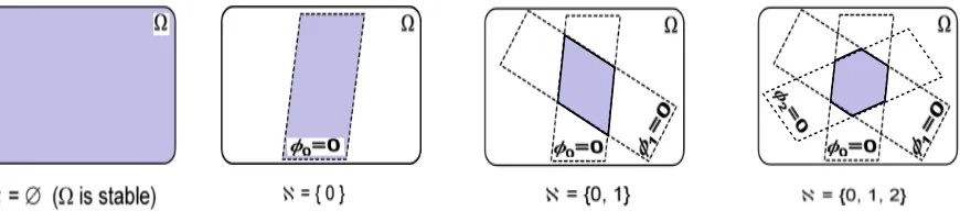
Denote ℵ={n: Re (λn)≥0}and (1)
ΩS= Ω if ℵ=∅ or ΩS= \
n∈ℵ
[φn = 0] if ℵ 6=∅
Then for a given regionσ⊆Ω, with non null measure, the system is σ-exponentially stable if and only if
meas (σ\ΩS) = 0 (8)
Proof: a)Suppose that (S) is exponentially stable onσ.
If ℵ=∅ then we obtain ΩS= Ω and then meas (σ\ΩS) = meas (σ∩ ∅) = 0. Now ifℵ 6=∅we know that there existsα >0 andM >0 such that
kχσz(t)k ≤M e−αtkz0k ∀t >0, ∀z0∈L2(Ω)
For alln∈ ℵwe have meas (σ∩[φn6= 0]) = 0,elsez0=φn givesz(t) =eλntφn and then
etRe(λn)kχ
σφnk ≤M e−αtkφnk , t >0 (9)
But in this casekχσφnk 6= 0 and (9) gives
e(Re(λn)+α)t≤M kφnk kχσφnk
, t >0
which is not satisfied whenttends to infinity because Re (λn) +α >0.
Then meas (σ∩[φn6= 0]) = 0,∀n∈ ℵ, and then
meas (σ\ΩS) = meas (σ∩ΩcS) = meas σ∩ [
n∈ℵ
[φn 6= 0] !!
= meas [
n∈ℵ
(σ∩[φn 6= 0]) !
≤X
n∈ℵ
meas (σ∩[φn 6= 0]) = 0
b)Reciprocally let σbe a given region with non null measure and satisfies (8). Ifℵ=∅, the system is exponentially stable and then it is alsoσ-exponentially stable. Ifℵ 6=∅, due to hypothesis 7,ℵhas a finite number of elements:
Denoten1= inf (ℵc). Thenℵ={0, , . . . n1−1}and
Re (λn1−1)>0>Re (λn1)>. . .
For everyn∈ ℵwe have meas (σ∩[φn6= 0])≤meas (σ∩Ωcs) = 0 and then χσφn= 0 almost ∂
χσzI(t) =
X
n∈ℵ
eλnthz
0, φniχσφn = 0
We deduce that for allz0∈X
kχσz(t)k
2
=kχσzS(t)k 2
6kzS(t)k2=X
n /∈ℵ
e2tRe(λn)hz 0, φni
2
≤e2tRe(λn1)X
n /∈ℵ
hz0, φni
2
≤e2tRe(λn1)kz0k2
with Re (λn1)<0 and then the system isσ-exponentially stable.
Remark 2.8. The condition meas (σ\ΩS) = 0 means thatσ⊆ΩS almost everywhere ; That is almost all the regionσis contained in ΩS (except a neglectable part).
We deduce from this theorem that when a given system is unstable (exponentially) the domain Ω can be divided on two regions: One region ΩS where the system is exponentially stable and another region Ωc
Figure 1. Zone of stability ΩS (grised zone) according toℵ.
where the system is exponentially stable and another region σ∩Ωc
S where the system is totally unstable. The figure 1 illustrates the different situations.
An extreme case is when meas (Ωc
S) = 0 (or Ω c
Sis empty) then the system is exponentially stable on all region with non null measure.
The other extreme case is when meas (ΩS) = 0 (or ΩS is empty), the system is then exponentially stable or else totally unstable. This is the case for systems of UTU type which are characterized by the following corollary:
Corollary 2.9. If A admits a system of orthonormal eigenfunctions (φn)n associated to eigenvalues (λn)n satisfying (7) then we have the equivalence:
(i) (S)is of UTU type ; (ii)meas (ΩS) = 0.
The corollary is deduced from theorem 2.7.
Remark 2.10. If meas [φn = 0] = 0 for allnthen the system is of UTU type but the converse is not true. It
is the case for example if there exists two eigenfunctionsφn1 andφn2 such that meas [φni = 0]6= 0 fori= 1,2
and meas T i=1,2
[φni= 0]
!
= 0: the system is of UTU type.
Remark 2.11. For distributed parameter systems, characterized by their spatiotemporal evolution, the space variable plays an important role. When A admits a system of orthonormal eigenfunctions (φn)n , associated
to eigenvalues (λn)n , the eigenfunctions φn(x) translates the effect of the eigenvalues λn through the domain
Ω (for exponential stability). This explains the fact that in the region σof Ω whereφn0(x) = 0, the effect (on stability) of the corresponding eigenvalue is not important in the sense that the system (S) can beσ-regionally exponentially stable either when<(λn0)≥0 (see figure 1).
As an application of the theorem 2.7, corollary 2.9 and remark 2.10 we have the two following examples.
Example 2.12. Consider the system described by the following state equation in Ω =]0,1[
∂z ∂t = α
∂2z ∂x2 + β
∂z
∂x Ω×]0, T[
z(0) =z0
z(0, t) =z(1, t) = 0
(10)
Using corollary 2.9, we deduce that the system is of UTU type because the corresponding eigenfunctions are given by [4]
φn(x) =
√
2 exp(−βx
2α) sin(nπx) Note that the corresponding eigenvalues are given by [4]
λn=−αn2π2−
β2
4α (11)
The system is totally unstable ifα <0 and exponentially stable ifα >0. Example 2.13. Consider the Haar system defined on Ω =]0,1[ by [1]
∂z(t)
∂t =Az(t) Ω×I
z(0) Ω
(12)
with for allz∈L2(Ω)
Az=λ1hz,1i+
X
(n,m)∈V
λ(n,m)
z, h(n,m)
h(n,m)
where V
={(n, m)∈N2 / m < 2n} and (λn,m)(n,m)∈V are real. h
(n,m)are the Haar’s functions defined for (n, m)∈V
andx∈Ω by
h(n,m)(x) =
2n/2 if x∈hm
2n,
m+1 2 2n
i
−2n/2 if x∈hm+12 2n ,
m+1 2n
i
0 elsewhere
(13)
The family {1, h(n,m)/(n, m) ∈ V}is an orthonormal basis of L2(Ω).
We notice for this example that for the eigenvalueλ1 the corresponding eigenfunction isφ1(x) = 1 forx∈]0,1[ and forλ0,0 the corresponding eigenfunctionh0,0(x)6= 0 for allx∈Ω =]0,1[. We consider the following case:
λ1=−π
λn,0=−(n+ 2)π if n≥0
λn,m=−(n+m+ 1)π if n <3, m6= 0
λn,m= 4−sup (n, m) if n≥3 andm6= 0
(14)
Then we have:
λn,m
= 1 if sup (n, m) = 3 = 0 if sup (n, m) = 4
6−1 if sup (n, m)<3 or sup (n, m)>4 Which gives:
ℵ={(3,1),(3,2),(3,3),(3,4),(4,1),(4,2),(4,3),(4,4)} As
[hn,m= 0] = i
0, m 2n h
∪
m+ 1
2n ,1
and
ΩS = \
(n,m)∈ℵ
[hn,m= 0] = 0, 1 16 ∪ 5
8,1
The system is not of UTU type and for all σ⊂
0,161
∪1 2,1
Remark 2.14.
(1) For systems of UTU type, there is equivalence between global and regional stability and consequently in this case the smallest disturbance that destabilizes the system destabilizes it totally (all regions are destabilized simultaneously).
(2) There exists systems which are not of UTU type (example (2.3) and example (2.13)). For such a systems we consider the regional stability radius problem.
3.
regional stability radius
Consider the system given by the following state equation defined on Ω⊂Rn
·
z(t) =Az(t) +Bu(t) t >0 z(0) =z0
(15)
Letσbe a subset of Ω with non null measure.
As we are interested by the state on the regionσ, we consider the regional output function given by :
yσ(t) =Cχ∗σχσz(t)
which can be written as follow: yσ(t) =C
σz(t) where χ∗σ is adjoint operator ofχσ and Cσ : ψ ∈ L2(Ω) →
Cχ∗σχσψ∈Y andC is given in (2).
We assume that (A, B, Cσ) is in the Pritchard Salamon class.
The solution of the disturbed system, in the case whereu(t) = Dyσ(t), whereD∈ D andDis a subset of L(L2Y, L2U), is given by:
z(t) =S(t)z0+
Z t
0
S(t−s)BDCσz(s)ds (16)
and the observation of the solutionz(t) onσis given by
yσ(t) =Cσz(t) =CσS(t)z0+Cσ Z t
0
S(t−s)BDCσz(s)ds (17)
Which gives
yσ=yσ0 +CσLDyσ (18)
whereyσ
0(t) =CσS(t)z0 and
L: L2(0,∞;U)→L2(0,∞;X) is defined by
(Lu) (t) =
Z t
0
S(t−s)Bu(s) ds (19)
We have the following definition
Definition 3.1. The regional stability radius (ofσ) of (18) is ˆ
ρσ(L, Cσ,D) = sup{d;r < d, implied∃Kr
such that sup
kDk≤r D∈D
kyσ(., D)kL2
Y ≤Krky
σ
0(.)kL2 Y}
Theorem 3.2. We have
b
ρσ L, Cσ,L L2Y,L
2
U
=kCσLk−1
Proof.The principle of the proof is the same as in Pritchard and Townley [7], but with taking into account the regional aspect. Indeed, ifkDk<kCσLk
−1
, thenkCσLDk<1 and thenCσLDis a contraction onL2Y and
then (18) admits a unique solution yσ(.)∈ L2
Y. Consider now a sequence u σ
n in L2U such that ku σ
nk = 1 and
kCσLuσnk=µσn is increasing toµσ=kCσLk. Lethσn= (µσ)−1CσLuσn andyσn=y0σ+ασnhσn where
ασn = h
1− khσnk
2i−1
hyσ0, hσni+ h
hyσ0, hσni
2
+1− khσnk
2
kyσ0k 2i12
(20)
Then we have kyσ
nk=αn andynσ∈L2Y for eachn.Put Dny= (uσnhynσ, yσi)/(µσkyσnk), then
(i)kDnk=kCσLk
−1
and (ii)kCσLDnk= µσn µσ <1. Then for each n, yσ
n is the unique solution ofyσ =y0σ+CσLDnyσ. As hσn = (µσ)−1Luσn, we choose uσn such
that hyσ
0, hσni ≥0.
And then from (20), we obtainkyσ
nk → ∞.
Definition 3.3. The regional stability radius ofσ, relatively toD ⊂ L(L2Y, L2U), is the greatest positive real r, denotedrσ(A, B, Cσ,D), such that for allD∈ Dthe solution of (16) isσ-exponentielly stable for eachz0inX.
The regional stability radius ofσis the greatest positive real r, notedrσ(A, B, Cσ), such that for all D∈ L
(Y, U),kDk< rthe solution of (16) isσ-exponentielly stable for eachz0in X.
That means that regional stability radius of σ (respectively relatively to D) is the smallest disturbance (relatively in D) that destabilizes the system on the regionσ.
For systems which aren’t of UTU we can also define the total stability radius as follow
Definition 3.4. The total stability radius of system (S), relatively toD ⊂ L(L2Y, L2U), is the greatest positive real r, noted rtotalD , such that for all D ∈ D, kDk < r, the solution of (16) (for each z0 in X) is not totally exponentially unstable.
The total stability radius of system (S) is the greatest positive real r, noted rD
total, such that for all D ∈
L(L2
Y, L
2
U),kDk< rthe solution of (16) (for each z0 onX) is not totally exponentially unstable.
That means that the total stability radius is the smallest disturbance which destabilizes totally the system. We have the result
Proposition 3.5. If we denote rΩthe global stability radius, then: 1. For all σ⊂ Ω,meas(σ)6= 0, we have rΩ ≤ rσ ≤ rtotal.
2. If the system is of UTU type, then ∀σ⊂Ω,meas(σ)6= 0,rΩ = rσ = rtotal. We have the same results for stability radius relatively to a given subsetD.
The proof lies with the fact that regional instability implies global instability and we have equivalence for the UTU systems.
To illustrate the regional stability radius we consider the following examples
4.
examples
Example 4.1. Consider the system described by the following state equation in Ω =]0,1[
∂z ∂t = α
∂2z ∂x2 + β
∂z
∂x + Bu ; Ω×]0, T[
z(0) =z0
z(0, t) =z(1, t) = 0
(21)
Augmented by the output function
y(t) =Cz(t) (22)
whereαandβ are a non null real.
In the autonomous case,u= 0, the system is of UTU type because the corresponding eigenfunctions are [4]
φn(x) =
√
2 exp(−βx
2α) sin(nπx)
Remark that the corresponding eigenvalue are given by [4]
λn=−αn2π2−
β2
4α (23)
Consider the case where the autonomous system is exponentially stable i. e. α > 0 and let us determine the stability radius of system (21) in two cases:
Case 1. Stability radius of system (21) relatively to a particular subsetDofL(L2
Y, L2U) forB=IandC=I .
We consider
D={Dγ∈ L(L2Y, L
2
U) defined byDγy=γy : γ∈R Dγ =γI} (24)
The disturbed system is then given by
∂z ∂t = α
∂2z ∂x2 + β
∂z
∂x +γz Ω×]0, T[
z(0) =z0
z(0, t) =z(1, t) = 0
(25)
The corresponding eigenfunction are given by [4]
φn(x) =
√
2 exp(−βx
2α) sin(nπx)
The nature of the corresponding eigenfunctions means that the system is of UTU type and consequently the total and regional stability radius are the same.
The corresponding eigenvalue are given by [4]
λn=γ−αn2π2−
β2
4α (26)
We have
r(A, I, I,D) =απ2+β 2
Case 2. We consider now the particular case whereα=−1,β= 0,Bu=δ(x−b)uandy(t) =Cz=hz, φn0i, we obtain [4]
G(iω)u=
* X
n
φn(b)u
iω−λn
φn, φn0
+
= φn0(b) iω−λn0
u (27)
Which gives forbsuch thatφn0(b)6= 0,
r(A, B, C) = |λn0| |φn0(b)|
(28)
As an example forb= 1+22nm
0 ,r(A, B, C) =
n20π2
√
2 .
For more details about the computation of the stability radius (and transfer functions) for different systems see Bernoussi [4].
Remark 4.2. As for the first case, the smallest disturbance that destabilizes the system destabilizes it totally (the system is of UTU type) and depends on the location (space) of the actuator but it depends also of the eigenfunctionλn0 for which the corresponding eigenfunctionφn0(x) =
√
2sin(n0πx) (meas{φn0(x) = 0} = 0). In the first case we have considered throughC=Iall the eigenvaluesλn(eigenfunctions φn) but in the second
case we have considered justλn0 (eigenfunctionsφn0).
We consider now an example where the operatorAadmits an orthonormal system of eigenfunctions but the system is not of UTU type: Example (2.13).
Example 4.3. Consider the Haar system given in example (2.13) but excited by a pointwise actuator located at pointb∈]0,1[
∂z
∂t =Az(t) + Bu(t) Ω × I
z(0) =z0 Ω
(29)
With for allz∈L2(Ω),
Az=λ1hz,1i+
X
(n,m)∈V
λn,m
z, h(n,m)
h(n,m)
whereV={(n, m)∈
N2 / m < 2n} and (λn,m)(n,m)∈V are reals.
We consider the case where (B=I,C=I) andDgiven by (24). The disturbed system is given by
∂z
∂t =Az(t) + γz(t) Ω × I
z(0) =z0 Ω (30)
In this case the corresponding eigenfunctions are 1 andh(n,m)given by (13) and the corresponding eigenvalues areλ1+γandλn,m+γ. We have the result
Proposition 4.4. 1. The stability radius relatively toD isr(A, I, I,D) =min(|λ1|,|λn,m|) 2. The total stability radiusrtotal(A, I, I,D) =|λ1|.
In the two examples given above we have considered the case where the operator A admits a system of orthonormal eigenfunction φn(x) associated to eigenvaluesλn. In the following example we consider another
Example 4.5. Consider the system given in example (2.3) but excited by controlBu.
(S)
˙
z(t) =a(x)z(t) +Bu(t) t >0
z(0) =z0
(31)
Augmented by the output function
y(t) =Cz(t) (32)
We consider Ω =]0,4[,a(x) =x−5,B=I andC=I.
Remark that for the autonomous system (u= 0), (31) is exponentially stable. Foru=Dy the system (31) becomes:
(S)
˙
z(t) = [(x−5) +D]z(t) 0< t < T
z(0) =z0
(33)
The system (33) will be stable (on all Ω) for allDsuch that: |D|<1 and the system isn’t exponentially stable forD= 1. SorΩ(A, B, C) = 1.
Analysis of regional aspect. We remark at first that the system (S) isn’t of UTU type. (S) is exponentially stable on the region wherex−5 +D <0.
Consider now the three following regions: σ1= [0,1],σ2= [1,2] andσ3= [2,4], then:
• Forσ3: forD such that|D|<1 the system is σ3 exponentially stable but forD = 1 the system isn’t σ3 exponentially stable. So the regional stability radius of σ3 isrσ3 = 1.
• Forσ2: forD such that|D|<3 the system is σ2 exponentially stable but forD = 3 the system isn’t σ2 exponentially stable. So the regional stability radius of σ2 isrσ2 = 3.
• Forσ1: forD such that|D|<4 the system is σ1 exponentially stable but forD = 4 the system isn’t σ1 exponentially stable. So the regional stability radius of σ1 isrσ1 = 4.
Remark 4.6.
(1) The smallest disturbance which destabilizes the system (S) (globally) is D = 1 and the smallest dis-turbance which destabilizes it totally is D = 5 and for all region σ ⊂Ω with meas(σ) 6= 0, we have 1≤rσ≤5. Remark that (S) isn’t of UTU type.
(2) For systems of UTU type we have equality: The smallest disturbance which destabilize the system globally destabilize it totally (destabilizes all regionσ⊂Ω with meas(σ)6= 0).
(3) We can find this results also by considering in (32) as a measure functionyσi=Cχ
σizfori= 1,2 and 3.
This example shows clearly the importance of regional stability radius for systems which are not of UTU type.
5.
conclusion
we have shown that there exists some systems which are not of UTU type (for which instability (global) is not equivalent to regional instability), and for which each zoneσ⊂Ω has its proper stability radius which could be calculated by a ”regional” measure. For such a systems it would be interesting to develop all the other problems of robust control through a regional aspect. For example as each zone σ⊂Ω has its own stability radius we can introduce the concept of vulnerability [3, 5, 17] to stability (A given zone σ1 will be ”more vulnerable to stability” than σ2 if its stability radiusrσ1 ≤rσ2). Consequently we can consider problems of robust control (optimal) through the ”more” vulnerable zone. Also it will be very interesting to consider time varying and non linear systems. Some of those problems are under investigation.
References
[1] L. Afifi, A. El Jai and E. Zerrik, 2008.Syst`emes dynamiques 2 : Analyse r´egionale des syst`emes lin´eaires distribu´es. Collection ´
etudes. Presse Universitaire de Perpignan.
[2] A. Bernoussi, 2009.Regional stability radius of distributed parameter systems. Proceeding Intenational confrence Systems Theory: Modelling, analysis and control. pp. 201-208. Collection ´etudes. Presse Universitaire de Perpignan.
[3] A. Bernoussi, 2007.Spreadability and vulnerability of distributed parameter systems.International Journal of Systems Science, Vol. 38, N. 4, April 2007, 305-317.
[4] A. Bernoussi, 1993.Approche Fr´equentielle des syst`emes Distribu´es - Relation avec les capteurs et les actionneurs. Th`ese de Doctorat, Universit´e de Perpignan, France.
[5] A. Bernoussi et M. Amharref, 2003.Etalabilit´e - vuln´erabilit´e.Annals of University of Craiova, Math. Comp. Sci. Ser. Volume 30, 2003, pp 53-62. ISSN 1223-6934.
[6] W. Desch and W. Shappacher, 1985.Spectral properties of finite dimensional perturbed linear semigroups. J. Differential Equations 59 (1985), 80-102.
[7] A. J. Pritchard and S. Townley, 1989.Robustness of linear Systems. Journal of Differentiel Equations. Vol. 77, No. 2, February 1989.
[8] A. J. Pritchard and S. Townley, 1986.A stability radius for infinite dimensional systems. In ”Infinite dimensional systems. Proc. Vorau” (F. Kappel, Ed), pp. 272-291. Springer-Verlag, New York/Berlin, 1986.
[9] D. Hinrichsen and A. J. Pritchard, 1986. Stability radii for linear systems. Systems control lett. 7, pp. 1-10.
[10] D. Hinrichsen and A. J. Pritchard, 1986.Stability radius forstructured perturbations and the algebraic Riccati equation. Systems Control lett. 8, No. 2, 105-113.
[11] A. El Jai, 2004.El´ement d’Analyse et de Contrˆole des syst`emes. Collection Etudes, Presses Universitaires de Perpignan, ISBN: 2-914518-60-9.
[12] A. E. Jai, M. C. Simon, and E. Zerrik, 1993.Regional observability and sensors structures. International Journal of Sensors and Actuators 39, 1993.
[13] A. E. Jai, M. C. Simon, E. Zerrik, and A. J. Pritchard. 1995. Regional controllability of distributed parameter systems. International Journal of Control 62, 1995. 43.
[14] R. Al-Saphory and A. E. Jai, 2002.Asymptotic regional state reconstruction. International Journal of Systems Sciences 33(13), pp. 1025-1037, 2002. 72.
[15] J. L. Lions, 1981Some methods in the mathematical analysis of systems and their control.Sciences Press. Beijing. China. [16] J. L. Lions and E. MagenesProbl‘emes aux limites non homog`enes et applications. Dunod. Paris. 1968.
[17] Y. Qaraai, A. Bernoussi and A. El Jai, 2007.How to control a spreadind disturbance for a class of non linear systems. Int. J. Appl. Math. Comput. Sci., 2008, Vol. 18, No. 2, 171-187. DOI: 10.2478/v10006-008-0016-9.